An observational and theoretical view of the radial distribution of HI gas in galaxies

Abstract

We analyze the radial distribution of HI gas for 23 disk galaxies with unusually high HI content from the Bluedisk sample, along with a similar-sized sample of ”normal” galaxies. We propose an empirical model to fit the radial profile of the HI surface density, an exponential function with a depression near the center. The radial HI surface density profiles are very homogeneous in the outer regions of the galaxy; the exponentially declining part of the profile has a scale-length of $\sim 0.18$ R1, where R1 is the radius where the column density of the HI is 1 $M_{\odot}$ pc^-2. This holds for all galaxies, independent of their stellar or HI mass. The homogenous outer profiles, combined with the limited range in HI surface density in the non-exponential inner disk, results in the well-known tight relation between HI size and HI mass. By comparing the radial profiles of the HI-rich galaxies with those of the control systems, we deduce that in about half the galaxies, most of the excess gas lies outside the stellar disk, in the exponentially declining outer regions of the HI disk. In the other half, the excess is more centrally peaked. We compare our results with existing smoothed-particle hydrodynamical simulations and semi-analytic models of disk galaxy formation in a $\Lambda$ Cold Dark Matter universe. Both the hydro simulations and the semi-analytic models reproduce the HI surface density profiles and the HI size-mass relation without further tuning of the simulation and model inputs. In the semi-analytic models, the universal shape of the outer HI radial profiles is a consequence of the assumption that infalling gas is always distributed exponentially. The conversion of atomic gas to molecular form explains the limited range of HI surface densities in the inner disk. These two factors produce the tight HI mass-size relation.

1 introduction

Over the last three decades, there have been many efforts to map the distribution of HI in galaxies using radio synthesis telescopes. The first analyses focused on massive and HI-luminous galaxies (e.g. Bosma 1978, Wevers et al. 1984). There were also surveys specifically focusing on galaxies in clusters (Warmels 1988, Cayatte et al. 1990, Verheijen & Sancisi 2001, Chung et al. 2009), which demonstrated that the HI is depleted as a result of tidal stripping by neighboring galaxies or ram-pressure stripping by the surrounding intracluster medium. WHISP (Westerbork observations of neutral Hydrogen in Irregular and SPiral galaxies, van der Hulst et al. 2001, Swaters et al. 2002) was one of the largest efforts to map the distribution of HI in different types of galaxies. The survey took nearly 10 years, observing around 500 galaxies with Hubble types from S0 to Im. From these studies, we have learned about the spatial and kinematic properties of HI in disk galaxies. The radial HI surface density profiles exhibit a wide variety of features attributable to irregularities in the galaxy such as spiral arms, rings, bars, warps etc. Studies of larger samples reveal basic scaling relations that provide hints of the mechanisms regulating the evolution of galaxies. In contrast to the stellar surface density, which is peaked in the center of the galaxy and drops steeply with radius, the radial distribution of HI often flattens or even declines near the center of the galaxy. In the outer regions, the HI disks usually extend to larger radius than the stellar disks and the profiles are well-fit by exponential functions. Studies of different types of galaxies reveal that they all obey the same tight HI size-mass relation (Broeils &Rhee, 1997; Verheijen & Sancisi, 2001; Swaters et al., 2002; Noordermeer et al., 2005). Recently, Bigiel &Blitz (2012) (hereafter B12) found for a sample of 32 nearby spiral galaxies, that the combined HI and $\rm{H_{2}}$ gas profiles exhibit a universal exponentially declining radial distribution, if the radius is scaled to R25, the optical radius of the galaxies.

Recently, in an attempt to understand gas accretion in galaxies, we used the Westerbork Synthesis Radio Telescope (WSRT) to map hydrogen in a sample of 25 very gas-rich galaxies, along with a similar-sized sample of “control” galaxies with similar masses, sizes and redshifts (Wang et al. 2013, Paper I). Thanks to improvements in the WSRT instrumentation and data analysis, we were able to reach significantly lower HI column densities than previous surveys, which have targeted (late-type) disk galaxies in the field. The sample is selected using physical properties such as stellar mass and HI mass fraction, and is thus well-suited for direct comparisons with theoretical models. In Paper I, we analyzed the sizes and morphologies of the HI disks. The HI-rich galaxies lie on the extension of the well-known HI mass-size relation (Broeils &Rhee, 1997) for normal spiral galaxies, and do not exhibit more irregular HI morphologies compared to the control galaxies. The conclusion is that major mergers are not likely to be the main source of the extra cold gas.

In this paper, we search for further clues about gas accretion by studying the radial HI surface density profiles of the galaxies in the sample. Again, we compare the HI-rich galaxies with the control sample. Our paper is organized as follows: section 2 describes the data used in this paper. In section 3, we present the radial profiles of HI and propose a model to describe the shape of the HI profiles. We present our major observational result that the galaxies exhibit a universal HI radial profile in the outer regions. In section 4, we estimate $\rm{H_{2}}$ profiles from the SFR profiles for comparison with the results of B12. We compare our empirical results with smoothed-particle hydrodynamics (SPH) simulations and semi-analytic models in section 5. We discuss the possible physical origin of our main observational results in section 6.

2 Data and previous work

The Bluedisk project was designed to map the HI in a set of extremely HI-rich galaxies and a similar-sized set of control galaxies, which are closely matched in stellar mass, stellar mass surface density, inclination and redshift. The aim is to search for clues about how galaxy disks grow as a result of gas accretion in the local universe. We refer the readers to Paper I for details on the sample selection, observations and initial data analysis. Here, we review the most relevant information. All galaxies that were observed have stellar massed above 10¹⁰ $M_{\odot}$, and redshifts between 0.01 and 0.03. All galaxies have optical photometry and spectroscopy from the Sloan Digital Sky Survey (SDSS, Abazajian et al., 2009) Data Release 7 spectroscopic MPA/JHU catalog and UV photometry from the DATA Release 5 of the Galaxy Evolution Explorer (GALEX) imaging survey (Martin et al., 2010). We have gathered or measured a variety of parameters describing the stellar component of the galaxies, including sizes (R50 the half-light radius, R90 the radius enclosing 90% of the light, and D25 the major axis of the ellipse where the $g$-band surface density reaches 25 mag arcsec^-2 ), stellar mass (M_∗), stellar mass surface density ($\mu_{*}=0.5M_{*}/\pi R50^{2}$), concentration index (R90$/$R50), colours and star formation rates (SFR) derived from SED (spectral energy distribution) fitting.

Following Paper I, the sample that will be used in this work includes 42 galaxies. 5 interacting (multi-source) systems, one strongly stripped system and one non-detection have been excluded. The analysis sample is divided into 23 HI-rich galaxies and 19 control galaxies, depending on whether the galaxy has more HI mass than deduced from its NUV-r color and stellar mass surface density using the relation given in Catinella et al. (2010, hereafter C10). As in Paper I, our results are derived from the HI total intensity images, for which we have produced detection masks and error images. We have measured the size R1 (the semi-major axis of the ellipse where the HI surface density reaches 1 $M_{\odot}\rm{pc^{-2}}$) for each galaxy. We have also parameterized the morphology of the HI disks using $A$, M20 and Gini from the concentration-asymmetry-smoothness (CAS) system (Lotz et al., 2004; Conselice, 2003), and 3 newly defined parameters that are more sensitive to irregularities in the outer parts of the HI disks, $\Delta$Center, $\Delta$PA and $\Delta$Area. The reader is referred to Paper I for more details.

3 A universal HI profile

3.1 Derivation of the angular averaged radial surface density profiles

We measure the angular averaged radial HI surface density profile along ellipses with position angle and axis ratio (a$/$b) determined from the SDSS r-band images. The sampling radius (semi-major axis of ellipses) increases linearly with a step of 1 pixel (4 arcsec, $\sim$ 2.8 kpc), which is smaller than the PSF, which is determined by the size of the synthesised beam in our data ($\sim$20 arcsec). In Paper I, we showed that the majority of the galaxies in our sample have surface density detection thresholds of 0.7$\times 10^{20}$ atoms cm^-2 at a S$/$N (signal-to-noise ratio) of 2. We can go deeper when averaging over a larger area, so we can typically measure the radial profiles out to an average surface density $\Sigma_{HI}$ of 0.2$\times 10^{20}$ atoms cm^-2. We do not include the helium gas in the HI-only analysis in this paper. The surface densities are corrected to be face-on by multiplying by cos$\theta\sim$ b$/$a, where $\theta$ is the inclination angle of the disk. We also divide the galaxy into two halves along the major axis and measure the radial HI surface density profile for each half. These profiles are displayed as one black and two grey curves in Fig. 1. We can see that the radial profiles for the two halves of the galaxy do not usually deviate much from the angular-averaged radial profile, for both HI-rich and control galaxies. In the following sections, we only focus on the angular-averaged HI radial surface density profiles (HI radial profiles for short hereafter). All the HI radial profiles decline exponentially in the outer regions and flatten or decline towards the central region, consistent with previous observations of nearby spiral galaxies (e.g. Wevers 1984, Swaters et al. 2002).

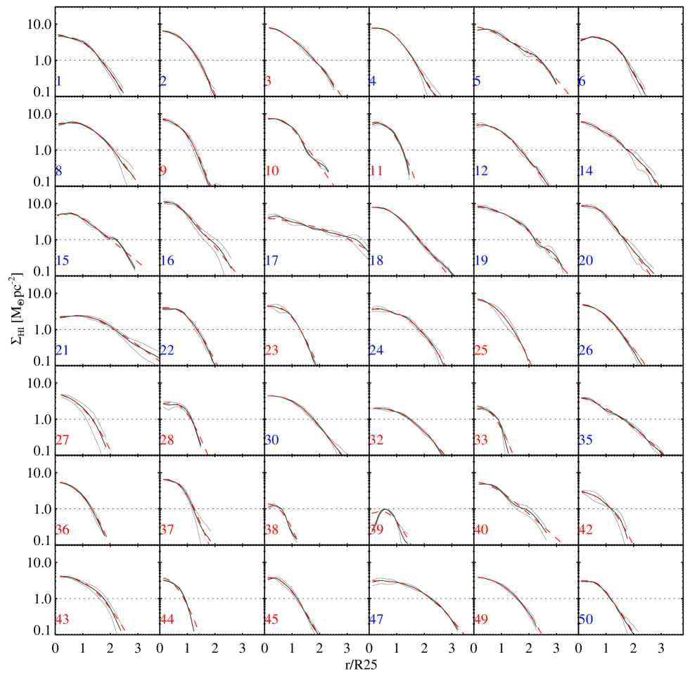
Figure 1: Radial profiles of the HI surface density for the 42 galaxies analyzed in this paper. The azimuthally averaged profiles are plotted in black, the profiles for each half of the galaxy divided along the major axis are plotted in grey, and the best-fit model fits (see section 3.2) to the profiles shown in black are plotted as red dashed lines. Intersection of the profiles with the dotted lines indicate where the HI surface density reaches 1 $M_{\odot}\rm{pc^{-2}}$. The ID of each galaxy is noted in the corner, coloured in blue for HI-rich galaxies and in red for control galaxies.

3.2 Model-fitting

It has often been remarked that the outer HI surface density profile follows an exponential form beyond the bright, star-forming stellar disk, while in the reach of the disk the surface density is more constant with a possible depression at the center (e.g. Swaters et al. 2002, Bigiel et al. 2012). To describe the shape of a two-component HI radial profile and to obtain the de-convolved shape of it, we choose a simple analytic expression of the form

$$\Sigma_{\rm HI,model}(r)=\frac{I_{1}\exp(-r/r_{\rm s})}{1+I_{2}*\exp(-r/r_{\rm c})},$$ (1)

and fit our data to it, where $I_{1}$, $I_{2}$, $r_{\rm s}$ and $r_{\rm c}$ are free parameters. When the radius is large, the denominator is equal to one and the function reduces to an exponential with scale radius $r_{\rm s}$. $r_{\rm c}$ is the characteristic radius where the profile transitions to the inner flat region. In this new analytic model, $I_{1}$ is likely to be connected with the HI$+\rm{H_{2}}$ total gas and $I_{2}$ is likely to be connected with the $I_{1}/I_{2}$ atomic-to-molecular gas conversion factor (Leroy et al. 2008). As we will show below, this model is very suitable to describe the radial distribution of HI surface density under the resolution of Bluedisk type.

We use the IDL code MPFIT (Markwardt, 2009), which performs least-squares curve and surface fitting. To achieve a fast and stable fit, the whole fitting procedure includes 3 steps.

1. The first step is to guess the initial value of the model parameters. We ignore the angular distribution of HI surface density in the HI image and the convolution effect of the beam, and simply perform a linear fit to the outer half of the HI radial profile. The slope and intercept distance of the linear fit are converted into initial guesses for $r_{s}$ and $I_{1}$. The initial $r_{\rm c}$ is set equal to 0.9 $r_{\rm s}$ and the initial $I_{2}$ is set equal to 9; these are the mean values of these parameters found by Leroy et al. (2008).

2. In the second step, we assume both the HI surface density distribution and the beam are azimuthally symmetric. With the initial parameters obtained in the last step, we build a model profile and convolve it with one-dimensional Gaussian function with a width of FWHM$\sim\sqrt{b_{\rm{min}}\times b_{\rm{maj}}}$, where b_min and b_maj are the minor and major axis (in FWHM) of the beam. The convolved profile ($\Sigma_{\rm{HI,model}}$) is compared with the observed profile. The MPFIT code then tunes the model parameters to find the best fit.

3. In the final step, we take into account the axis ratio and position angle of both the galaxy and the beam in the HI image. The best-fit model parameters from the second step are used as initial input. We build a model image with the observed axis ratio and position angle of the galaxy. The model image is then convolved with the beam. We measure the radial profiles ($\Sigma_{\rm{HI,model}}$) from the convolved model image in the same way as they are measured from the observed HI image (Sect. 3.1). The simulated profiles are compared to the observed HI radial profile. The MPFIT code is then used to tune the model parameters to find the best-fit.

The best-fit model profiles are displayed as red dashed lines in Fig. 1. We can see that in general the model describes the observed profiles very well.

We now estimate errors for our derived parameters, as well degeneracies in the fits. We construct a grid around the best-fit parameters: $r_{\rm s}$ and $r_{\rm c}$ vary with a step size of 0.02 R25 in a range $\pm$R25 about the best-fit values, while and $I_{1}$ and $I_{2}$ vary with step size of 0.01 dex in a range $\pm$1 dex about the best values. We calculate the sum of square residuals between the convolved model and the data at each grid point

$$\kappa^{2}=sum(\frac{(\Sigma_{\rm{HI,model}}-\Sigma_{\rm{HI}})^{2}}{\sigma(\Sigma_{\rm{HI}})^{2}}),$$ (2)

and take $p_{i}=$exp(-$\kappa^{2}/2$) as the goodness-of-fit of the parameters for modelling the data at the grid point $i$. We thus build a probability distribution function (PDF) within the parameter grids by assigning $p_{i}$ as the relative probability of the data to be modelled by the parameters at grid $i$. We project the PDF in the direction of each parameter, and find the contours that contain 99.5 percent of the cumulative probability distribution. The half-width of these contours correspond to 3 times $\sigma$ (error) of the parameter. The derived errors for the whole sample are listed in Table 1 (and displayed as a histogram in Fig. 2). We summarize our results as follows:

1. $r_{\rm s}$ is well constrained ($\sigma<$ 1 kpc) for most of the galaxies in the Bluedisk sample.

2. $r_{\rm c}$ often has large error bars ($\sigma>$2 kpc), due to the resolution limit of the HI images.

3. There is strong degeneracy between $I_{1}$ and $I_{2}$ for all the galaxies, the 1 $\sigma$ errors for both $I_{1}$ and $I_{2}$ are larger than 0.3 dex.

4. $I_{1}/I_{2}$ can be well-constrained with $\sigma\sim$0.2 dex for nearly half of the galaxies, but when the HI disks are relatively small (R${}_{1}<$30 arcsec), $I_{1}/I_{2}$ cannot be robustly determined and has large errors.

We test our method with galaxies from the WHISP survey (Swaters et al., 2002) to ensure that our estimates of $r_{\rm s}$ will not be compromised by the resolution of Bluedisk HI images. We select the galaxies with optical images available from the SDSS and with stellar masses greater than 10^9.8 M_⊙. The publicly available total-intensity maps of the WHISP galaxies (with a median distance of z$\sim$0.008) are rescaled in angular size so that they have similar dimensions to the Bluedisk galaxies (with median distance of z$\sim 0.026$), and convolved with a Gaussian PSF of 22$\times$16 arcsec². We fit the model to the HI profiles from both the original WHISP images and the rescaled images. We compare these two estimates of $r_{\rm s}$ in Fig. 3. The two estimates correlate with a correlation coefficient of 0.7 and there is no systematic offset. The scatter around the 1-to-1 line is 3.3 kpc, larger than the error listed in Table 1, because the WHISP data is much shallower than the Bluedisk data.

ID	$r_{\rm s}$	$\sigma_{rs}$	$r_{\rm c}$	$\sigma_{rc}$	$I_{1}$	$\sigma_{I1}$	$I_{2}$	$\sigma_{I2}$
	kpc	kpc	kpc	kpc	$M_{\odot}\rm{pc^{-2}}$	dex	$M_{\odot}\rm{pc^{-2}}$	dex
1	6.91	0.64	6.35	0.74	181.15	0.68	23.80	0.61
2	3.95	0.40	3.91	0.51	760.45	0.64	35.73	0.57
3	4.69	0.41	7.02	1.31	335.88	0.72	13.25	0.68
4	7.20	0.61	3.58	0.55	113.87	0.62	11.18	0.52
5	6.17	0.98	8.78	2.97	1162.44	0.69	79.04	0.65
6	7.83	0.60	6.32	0.40	310.51	0.80	45.73	0.77
8	7.84	0.74	5.79	0.75	64.62	0.67	9.94	0.55
9	3.62	0.38	3.28	0.73	1060.26	0.69	65.03	0.63
10	6.53	0.66	2.54	1.14	26.31	0.68	7.33	0.72
11	4.23	0.36	2.75	0.48	461.41	0.76	84.26	0.72
12	8.50	0.93	5.69	2.21	72.57	0.68	6.10	0.67
14	8.27	1.21	12.14	6.09	245.10	0.60	11.96	0.73
15	22.32	1.63	7.48	2.82	14.66	0.57	2.34	0.47
16	5.86	0.39	0.66	0.19	31.13	0.16	43.32	0.76
17	7.71	2.24	9.36	0.25	476.54	0.11	62.71	0.76
18	8.52	0.63	1.48	1.10	68.59	0.66	60.54	0.59
19	7.47	1.00	7.45	3.60	124.83	0.69	9.22	0.68
20	7.15	0.47	1.74	0.69	48.02	0.59	17.51	0.49
21	9.10	0.84	1.95	1.08	20.93	0.68	63.86	0.70
22	5.45	0.51	3.13	0.52	305.92	0.70	47.68	0.65
23	5.12	0.45	3.59	0.87	365.23	0.72	53.47	0.69
24	7.46	0.61	7.74	0.81	230.00	0.73	24.98	0.70
25	4.11	0.58	4.56	3.79	224.27	0.69	16.37	0.66
26	2.99	0.24	2.05	0.41	540.47	0.73	43.68	0.73
27	1.85	0.45	1.26	2.15	385.18	0.75	67.09	0.62
28	3.32	0.35	2.01	0.40	52.62	0.70	33.62	0.76
30	6.51	0.64	4.31	1.03	440.29	0.69	34.81	0.62
32	3.12	0.25	2.28	0.43	272.01	0.70	75.07	0.68
33	2.95	0.54	1.79	0.54	81.20	0.70	38.89	0.75
35	7.92	0.66	14.15	0.23	579.77	0.07	23.17	0.77
36	2.45	0.40	1.62	2.00	334.37	0.71	60.83	0.72
37	3.53	0.39	1.93	0.52	147.55	0.67	38.81	0.71
38	2.69	0.78	1.44	3.00	38.32	0.78	50.66	0.75
40	7.56	0.74	0.47	0.21	13.43	0.13	66.24	0.76
42	3.53	0.78	3.80	3.33	216.74	0.76	29.05	0.59
43	3.18	0.32	2.77	0.74	332.24	0.70	57.64	0.66
44	2.24	0.30	1.47	0.35	268.87	0.75	59.20	0.77
45	3.40	0.32	1.97	0.82	334.05	0.70	64.08	0.64
47	6.50	0.91	6.25	1.38	318.16	0.69	53.31	0.62
49	3.80	0.37	3.77	0.66	688.92	0.72	74.17	0.69
50	5.18	0.57	3.02	1.32	464.34	0.69	73.66	0.63

Table 1: Parameters of the best-fit models for the HI radial profiles.

Figure 2: Distribution of errors on the parameters,$r_{\rm s}$, $r_{\rm c}$, $I_{1}$, $I_{2}$ and $I_{1}/I_{2}$ in the best-fit models for the HI radial profiles.

Figure 3: WHISP galaxies are shifted and convolved with the WSRT beam to have similar appearance to the Bluedisk galaxies. $r_{\rm s}$(shift) are the scale-length measured from the shifted and convolved images, and $r_{\rm s}$(expected) are the true scale-length expected at the redshifts of the Bluedisk galaxies. The crosses show the sizes of the Bluedisk galaxies.

3.3 The universal HI radial profiles in outer disks

We divide the Bluedisk sample into 3 equal sub-samples by their stellar properties (stellar mass, stellar mass surface density, colour, and colour gradient) and HI properties (HI:optical size ratio, HI mass fraction, HI mass, deviation from the C10 plane (,see section 2), and the morphological parameters $\Delta$Area and $\Delta$Center). Instead of scaling the profiles by R25, the characteristic optical radius of the disk, we scale by R1, the radius where the column density of the HI is 1$M_{\odot}$ pc^-2. The median HI radial profiles of the sub-samples are displayed in Fig. 4. The outer HI profiles now display “Universal” behaviour and exhibit an exponentially declining profile from $\sim$0.75 R1 to 1.3R1. Even the HI-rich galaxies (with large $\Delta\rm{f_{HI}}$), which were postulated by C10 to have experienced recent gas accretion, the clumpy HI disks with large $\Delta$Area, or HI disk that are off-center with respect to the optical disk (with large $\Delta$Center), have outer HI profiles that do not deviate significantly. We note that the median value of the averaged surface between 0.75 R1 and 1.25 R1 is $\sim 1.142\pm 0.022M_{\odot}\rm{pc^{-2}}$.

The differences between the inner profiles (at radii smaller than 0.75 R1) are much more prominent. They are most significant when the sample is split by NUV-r colour. In the next sections, we will show that in semi-analytic models that treat the conversion of atomic gas into molecular gas, differences in the inner HI surface densities arise because the gas reaches high enough surface densities in the central region of the galaxy to be transformed into molecular form. Because the level of star formation activity in the galaxy is tied to its molecular gas content, correlations between star formation rate and HI surface density will arise naturally.

In Fig. 5, we plot the best-fit model profiles rather than the actual profiles. We can see that the results in the outer regions of the disks do not change. The median $\Sigma_{\rm{HI,0.75-1.25R1}}$ from the best-fit models is $\sim$1.083$\pm$0.063 $M_{\odot}\rm{pc^{-2}}$. We plot the ratios $r_{\rm s}$/R1 and $r_{\rm s}$/R25 as a function of HI mass fraction in Fig. 6. From the left panel, we can see that the dispersion of $r_{\rm s}$/R1 around the median value of 0.19$\pm$0.006 is small. There are 2 HI-rich galaxies (galaxy 15 and 21) and one control galaxy (galaxy 40) which deviate from the mean $r_{\rm s}/$R1 by more than 0.1. These galaxies were not peculiar in terms of their HI mass (fractions), morphologies, global profiles, nor did their tellar properties differ in any clear way from the other galaxies in the sample.

From the right panel of Fig. 6, we can seen that $r_{\rm s}/$R25 spans a much wider range of values, from 0.15 to 0.8, with most of the values below 0.6. The HI-rich galaxies have systematically higher HI-to-optical size ratios and also span a larger range in values.

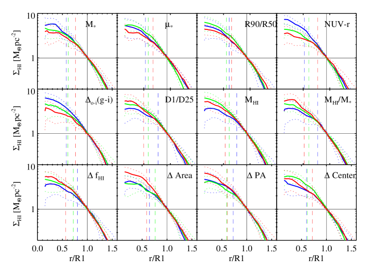
Figure 4: The galaxy sample is equally divided into 3 sub-samples according to the parameter denoted at the top right corner of each plot. These include stellar mass (M_∗), stellar mass surface density ($\mu_{*}$), concentration index (R90$/$R50), NUV–$r$ colour, colour gradient ($\Delta_{o-i}(g-i)$), HI-to-optical size ratio (D1$/$D25), HI mass ($M_{\rm{HI}}$), HI mass fraction ($M_{\rm{HI}}/M_{*}$), HI excess ($\Delta\rm{f_{HI}}$), and HI morphological parameter $\Delta$Area, $\Delta$PA, and $\Delta$Center. The median HI profile for each sub-sample is plotted in blue for the lowest values of each parameter, in red for the highest values and in green for intermediate values. The dotted lines show the scatter arround the median profiles. The dashed lines show the median value of R25$/$R1 for each of the sub-samples . The solid lines indicate R$1=1$ and $\Sigma_{\rm{HI}}=1M_{\odot}\rm{pc^{-2}}$.

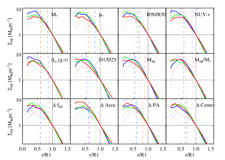
Figure 5: Similar as Fig. 4, but for the best-fit model profiles.

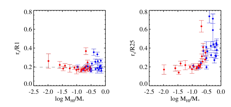
Figure 6: $r_{\rm s}$/R1 (left) and $r_{\rm s}$/R25 (right) are plotted as a function of HI mass fraction. The black dashed line shows the median value of $r_{\rm s}/$R1. HI-rich galaxies are plotted in blue, while control galaxies are plotted in red.

3.3.1 Relation to the HI mass-size relation

It is well known that in disk galaxies, the HI mass and the HI size R1 are tightly correlated (Broeils &Rhee, 1997; Verheijen & Sancisi, 2001; Swaters et al., 2002; Noordermeer et al., 2005, and Paper I). (Broeils &Rhee, 1997) parametrize this relation as

$$\frac{{{M_{{\rm{HI}}}}}}{{{M_{\odot}}}}=\left({12.88\pm 3.85}\right){\left[{\frac{{R1}}{{{\rm{pc}}}}}\right]^{2}}$$ (3)

Our finding that the HI gas in the outer region of disks has a ”universal” exponential surface density profile offers a natural explanation for the tight HI mass-size relation. Our results also suggest that similar tight relations should be found for different definitions of HI size. This is illustrated in Fig. 7, where we show the correlations between $M_{\rm{HI}}$ and the radii where the HI surface density reaches 0.5, 1, 1.5 and 2 $M_{\odot}\rm{pc^{-2}}$, respectively. As can be seen, the correlations are equally strong and tight for all four radii. The scatter in the HI mass-size relation only increases significantly at radii coreesponding to surface densities greater than a few $M_{\odot}\rm{pc^{-2}}$, where the total cold gas content is expected to be dominated by molecular rather than atomic gas.

Figure 7: The relation between HI mass and the diameters of HI disks measured at a surface density of 0.5, 1, 1.5 and 2 $M_{\odot}\rm{pc^{-2}}$. The correlation coefficient $\rho$ is denoted in the corner of each figure. The dashed line shows the HI mass-D1 relation from Broeils et al.(1997).

3.3.2 Where is the “excess” HI gas located?

In this section, we subtract the median HI profile of galaxies in the “control” sample from the HI profile of each HI-rich galaxy, in order to study the spatial distribution of the excess gas. Results are shown in Fig. 8. Interestingly, there appear to be one class of galaxy (e.g. 2,3, 16, 14, 4, 18,20,5, 19) where the excess rises montonically towards the smallest radii, or peaks well within the optical radius R25. In a second class of galaxy (e.g. 22, 35, 47, 24,1 12, 15, 6, 30, 8, 17), the excess peaks very close to R25 and drops off on either side. The latter is suggestive of recent accretion of a ring of gas at the edge of the optical disk.

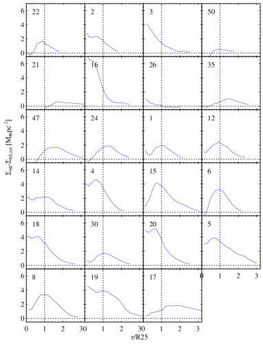
Figure 8: The difference between the HI profiles for the HI-rich galaxies and the median HI profile of the control galaxies. The dashed lines show where the radius equals R25. The IDs of the HI-rich galaxies are denoted in the corner of each panel.

4 The total cold gas profiles

B12 analyzed average gas radial distributions of 17 star-forming massive disk galaxies. They found that if they re-normalized the surface densities by dividing by the transition surface density $\Sigma_{\rm{transit}}$ where $\Sigma_{\rm{H_{2}}}$ equals $\Sigma_{\rm{HI}}$, and dividing the radii by R25, the characteristic optical radius of the disk, the resulting gas radial profiles exhibited a “Universal” exponential distribution beyond 0.2 R25, which could be parameterized as:

$$\Sigma_{\rm{gas}}/\Sigma_{\rm{transit}}=2.1e^{-1.65\rm{r/R25}}$$ (4)

In this section we explain how we construct total cold gas radial profiles for our Bluedisk galaxies, for comparison with the B12 results. We do not have information about the molecular gas in all the Bluedisk galaxies, and the spatial resolution of the Bluedisk HI data (FWHM of PSF $\sim$ 10.6 kpc) is lower than the B12 data (FWHM of PSF $\sim$ 1 kpc).

First, we use the star formation rate radial profiles to provide an estimate of the $\rm{H_{2}}$ radial profiles for our galaxies. We use the GALEX FUV images and the WISE 22 $\mu$m images to derive the SFR profiles ($\Sigma_{\rm{SFR}}$). The FUV images were converted to the resolution of the 22 $\mu$m images. Following Wright et al. (2010) and Jarrett et al. (2011), we apply a colour correction to the 22 $\mu$m luminosity of extremely red sources. We calculate the IR-contribution to the star formation rate (SFR_IR) of our sample by adopting the relation between SFR and WISE 22 $\mu$m luminosity in Jarrett et al. (2013). We adopt the formula from Salim et al. (2007) to derive the UV contribution to the star formation rate, SFR_FUV. The final SFR is the sum of SFR_IR and SFR_FUV. $\Sigma_{\rm{SFR}}$ is then converted into an estimated $\rm{H_{2}}$ surface density using the formula in Bigiel et al. (2008). The total gas radial profile is calculated as

$$\Sigma_{\rm gas}=1.36(\Sigma^{\prime}_{\rm{H_{2}}}+\Sigma_{\rm HI}),$$ (5)

where the factor of 1.36 corrects for the contribution from helium.

To confirm that this technique is robust, we apply it to the sub-sample of galaxies from the WHISP survey, which have GALEX NUV and WISE 22 $\mu$m images. Following the sample definition in B12, we select massive (M${}_{*}/M_{\odot}>10^{9.8}$), relatively face-on (size ratio b$/$a$>$0.5, or inclination angle smaller than 60 deg) star forming (NUV–$r<$3.5) disk (concentration $R90/R50<2.8$) galaxies. The WISE 22 $\mu$m images have similar resolution to the B12 images. The HI images of the WHISP galaxies have a FWHM PSF of $\sim$2 kpc, again very similar to that of the B12 images. The black points in the top panel of Fig. 9 show the average, scaled cold gas radial surface density profile. The relation derived by B12 is shown in orange, and the agreement is very good.

Following B12, to minimize resolution effects, the analysis is performed on the relatively face-on (b$/$a$>$0.5) Bluedisk galaxies, which include 12 HI-rich galaxies and 14 control galaxies. We note that the HI maps of the Bluedisk galaxies have considerably worse resolution (FWHM of PSF $\sim$ 10 kpc) than the B12 gas maps. We use the best-fit model HI profiles derived in the last section, instead of the directly-measured HI radial profiles. Because $\Sigma_{\rm{transit}}$ varies little from galaxy to galaxy, we assume a fixed $\Sigma_{\rm{transit}}\sim$ 14 $M_{\odot}\rm{pc^{-2}}$ from the B12 relation (Leroy et al. 2008) rather than calculating $\Sigma_{\rm{transit}}$ from the best-fit model HI profile. This is because the fit in the inner region has large uncertainties (section 3.2). Our results are shown in the middle and bottom panels of Fig. 9. From the middle panel of Fig. 9, we see that within 2R25 the mean gas profile of the Bluedisk sample is also consistent with the B12 relation. The individual profiles exhibit a large scatter around the B12 relation in the outer regions (beyond R25). In the bottom panel of Fig. 9, we plot the mean gas profile of the control galaxies in red and the mean profile of the HI-rich galaxies in blue. The mean profile of the HI-rich galaxies lies slightly above the B12 relation, while that of the control galaxies lies significantly below the B12 relation. This is consistent with our previous findings (Paper I) that HI-rich galaxies have larger R1$/$R25 than the control galaxies.

To summarize , the radial gas profile of Bluedisk galaxies exhibit large scatter around the B12 relation in their outer regions. The control galaxies deviate significantly from the B12 relation, which may be connected with the low accretion rate of cold gas or more evolved HI disks.

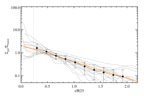
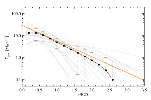
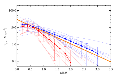
Figure 9: Top panel: estimated total gas profiles for the WHISP galaxies (grey). The black points show the average profile and the error bars indicate the 1$\sigma$ scatter derived from boot-strapping. The orange line shows the universal relation obtained by B12 when interacting systems are excluded. Middle panel: similar to the top panel, but for the Bluedisk galaxies. A fixed transition surface density $\Sigma_{\rm{transit}}\sim$ 14 $M_{\odot}\rm{pc^{-2}}$ is assumed (Leroy et al. 2008). Bottom panel: The same as the middle panel, except that the red lines are for the control galaxies and the blue lines are for the HI-rich galaxies.

5 Comparison with SPH simulations and Semi-Analytic Models

In this section, we will compare the results presented in the previous sections with the SPH simulations of Aumer et al. (2013) and the semi-analytic models of Fu et al. (2013).

5.1 Comparison with SPH simulations

We compare our observed HI profiles to those found in 19 $z=0$ galaxies from cosmological zoom-in SPH simulations. The simulations were described in detail in Aumer et al. (2013) and follow the formation of galaxies in haloes with masses $1\times 10^{11}<M_{200}/M_{\odot}<3\times 10^{12}$ in a $\Lambda$ Cold Dark Matter universe. The simulations include models for multiphase gas treatment, star formation, metal enrichment, metal-line cooling, turbulent metal diffusion, thermal and kinetic supernova feedback and radiation pressure from young stars. They lack, however, a model for the partition of atomic and molecular gas in interstellar medium.

As was shown in Aumer et al. (2013), the $z=0$ model galaxies all contain gas disks, with gas fractions that are higher than the observed average at the same stellar mass. The model disk galaxies are thus quite comparable in HI content to the Bluedisk galaxies. To obtain HI profiles for the simulated disks, we apply a simple model based on the observationally motivated model by Blitz & Rosolowsky (2006). The same model was used in the semi-analytic models of Fu et al. (2010).

We first select all gas with $T<15000\;\rm{K}$ and determine its angular momentum vector to orient the galaxy in a face-on orientation. We then divide the galaxies into quadratic pixels with $500\;\rm{pc}$ side-length. According to Blitz & Rosolowsky (2006) the ratio of molecular and atomic hydrogen is

$$f_{\rm mol}(x,y)=\Sigma_{\rm H_{2}}(x,y)/\Sigma_{\rm HI}(x,y)=\left(P(x,y)/P_{0}\right)^{\alpha},$$ (6)

where $\alpha=0.92$ and $P_{0}=5.93\times 10^{-13}\;{\rm Pa}$ are constants fit to observations. For the mid-plane pressure $P(x,y)$ we use the relation given by Elmegreen (1993),

$$P(x,y)={{\pi}\over{2}}G\left[\Sigma_{\rm gas}(x,y)^{2}+f_{\sigma}(x,y)\Sigma_{\rm gas}(x,y)\Sigma_{\rm stars}(x,y)\right]$$ (7)

, with the ratio of gas-to-stellar velocity dispersions

$$f_{\sigma}(x,y)={{\sigma_{\rm gas}(x,y)}\over{\sigma_{\rm stars}(x,y)}},$$ (8)

which, as the surface densities, we take directly from the simulations. To account for ionized hydrogen among the $T<15000\;\rm{K}$ gas, we assume a 25% ionized fraction in stellar dominated regions and correct for the absence of stars as a source of ionization by crudely invoking a factor $\Sigma_{\rm gas}/\Sigma_{\rm stars}$ where stars are sub-dominant.

The resulting HI surface density $\Sigma_{\rm HI}(x,y)$ is then used to create face-on HI profiles $\Sigma_{\rm HI}(r)$ for all model galaxies. $R1$ is then determined as the radius, where $\Sigma_{\rm HI}(r)$ drops below $1\;M_{\odot}\rm pc^{-2}$ and the HI mass $M_{\rm HI}$ as the total mass out to the radius, where $\Sigma_{\rm HI}(r)$ drops below $0.2\;M_{\odot}\rm pc^{-2}$, which corresponds to the detection threshold of the Bluedisk sample. To consider the effect of beam smearing in observations, we convolve $\Sigma_{\rm HI}(x,y)$ with an elliptical Gaussian Kernel with FWHM values of 14 and 9 kpc for major and minor axes. From the convolved surface density $\Sigma_{\rm HI,smooth}(x,y)$, we then derive $\Sigma_{\rm HI,smooth}(r)$, $M_{\rm HI,smooth}$ and $R1_{\rm smooth}$.

5.1.1 Results of the SPH simulation

The results of a comparison between simulations and observations are depicted in Fig. 10.

In the upper-left panel we depict the HI-to-stellar mass ratio $M_{\rm HI}/M_{\rm stars}$ as a function of stellar mass $M_{\rm stars}$ for the simulated and observed galaxies. The simulations (red) span a wider range in stellar mass ($9.5<\log(M_{\rm stars}/M_{\odot})<11.3$) than the observations which were limited to $10.<\log(M_{\rm stars}/M_{\odot})<11$. In terms of gas-richness, by construction about half of the observed galaxies lie above the black dashed line which depicts the median relation found by C10 (solid black line) shifted up by 0.6 dex. Only 4 of 19 simulated galaxies are above this line. The remaining simulated galaxies have a similar distribution of HI-mass fraction as the control sample, which have lower gas fractions.

In the upper-right panel of Fig. 10 we depict the HI mass-size relation. For the observed galaxies, we use D1 values corrected for beam-smearing effects and for simulated galaxies, we use un-convolved values. We see that the observed and the simulated samples both follow the relation found by Broeils &Rhee (1997). The agreement between the simulations and the observations is very good . The simulations show a very mild offset to lower HI masses, which may be connected to the difference in gas fraction of the samples or a minor problem of the HI modeling. Note also that the range of sizes of the galaxies in the two samples is very similar. We find that the largest HI disks in simulations form from gas that cools and settles in a disk after merger events at $z\sim 1$.

In the lower-left panel of Fig. 10 we depict a compilation of all 19 beam-convolved simulated HI-mass profiles $\Sigma_{\rm HI,smooth}(R)$ with radius $R$ in units of $R1$. All profiles have similar shape. They are rather flat in the centre and fall exponentially at $R>0.75\;{\rm R1}$. The central values in surface density scatter between 2 and 5 $M_{\odot}\rm pc^{-2}$, the outer exponential scale-lengths are between 0.15 and 0.45 $R1$. We overplot with diamonds the observed median profile of the Bluedisk galaxies and note that there is good agreement between simulations and observations.

The lower-right panel shows a comparison between the observed and the simulated median profiles. The central surface densities in simulations are slightly lower than in the observations, consistent with the slightly lower HI gas fractions in the top left panel . The outer profile at $R>0.5\;{\rm R1}$ agrees very well with the observations. We also note that the median outer HI scale-length of the un-convolved simulated disks is 0.17 in units of $R1$, which compares well to the beam-corrected mean value of 0.19 found for the Bluedisk sample. The dashed green and black curves show the median profiles we obtain , when we use the offset of the HI-to-stellar mass ratio of the simulated galaxies from the solid black line in the upper-left panel of Fig. 10 to equally divide the simulated sample into a gas-rich (green) and a gas-poor (black) subsample.

The dashed green and black curves show the mean profiles for simulated galaxies divided by HI-to-stellar mass. Simulated galaxies falling above the dashed black line in the top left panel are included in the “gas-rich” sub-sample, while those falling below this line are included in the “gas-poor” sub-sample.

We find that the gas-rich sample has higher central surface densities and shows steeper decline at the outer radii compared to the gas-poor sample. This differs from the observation that gas-richness has no influence on the outer slope. We caution however that we are looking at two samples with $\sim 10$ objects each. Considering the corresponding statistical errors there is no significant disagreement between the outer slopes. Moreover, if we use means instead of medians , the difference in outer scale-length becomes very small.

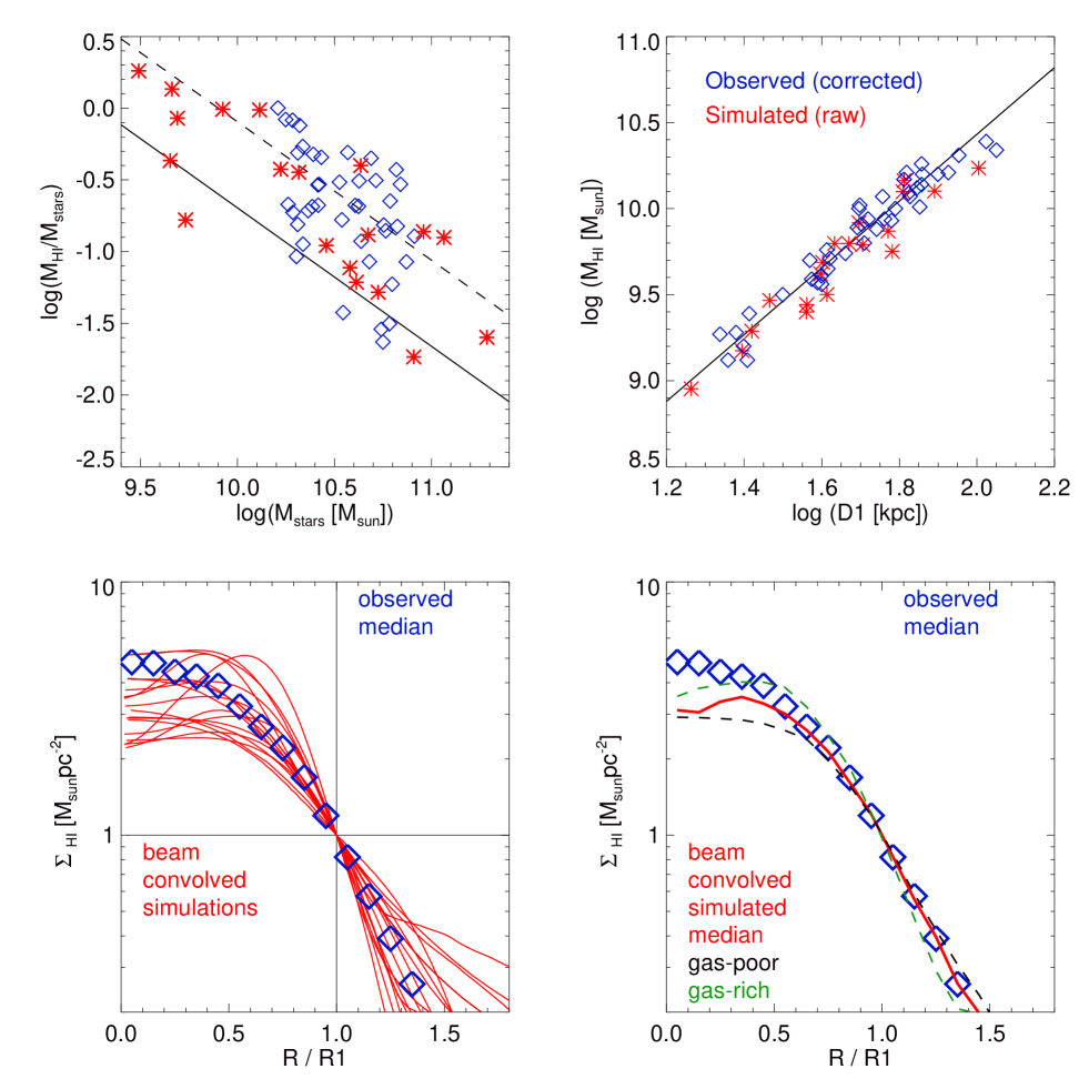
Figure 10: A comparison of the SPH simulations and the Bluedisk observations. Panel 1: The HI-to-stellar mass ratio $M_{\rm HI}/M_{\rm stars}$ as a function of stellar mass $M_{\rm stars}$ for simulated (red stars) and observed galaxies (blue diamonds). The solid black line shows the median relation between HI mass fraction and stellar mass found by C10, the dashed black line is offset from this relation by +0.6 dex. Panel 2: The HI mass-size relation. For simulations (red stars) we plot $M_{\rm HI}$ and $D1=2\;{\rm R1}$ determined from the un-convolved profiles, for observations (blue diamonds) we plot values that were corrected to account for beam effects. Overplotted in black is the relation found by Broeils &Rhee (1997). Panel 3: HI mass profiles for radii normalized to $R1$. We plot the convolved profiles $\Sigma_{\rm HI,smooth}(r)$ for all 19 simulated disks (red lines). We overplot the observed median profile (blue diamonds). Panel 4: As Panel 3, but now we compare the simulated median profile (red line) to the observed median profile (blue diamonds). We also show the medians for a gas-rich (green dashed) and a gas-poor (black dashed) sub-sample.

5.2 Comparison with semi-analytic models

In this section, we compare the observations with the semi-analytic models of galaxy formation of Fu et al. (2013; hereafter Fu13). In these models, each galaxy disk is divided into a series of concentric rings to trace the radial profiles of stars, interstellar gas and metals. Phyical prescriptions are adopted to partition the interstellar cold gas into atomic and molecular phases. In order to take into account the effects of beam smearing in the observations, the model radial profiles of $\Sigma_{\rm HI}$ are convolved by a Gaussian function with FWHM=10.6 kpc. The radius $R1$ is then derived from these smoothed profiles. In order to carry out as fair a comparison with the observations as possible, we select the galaxy with $\log_{10}[M_{\rm HI}/M_{\odot}]>9.0$, $10.0<\log_{10}[M_{\rm HI}/M_{\odot}]<11.0$ and $-1.8<\log_{10}[M_{*}/M_{\rm HI}]<0.2$ from the model sample at $z=0$.

5.2.1 Results from the Semi-analytical model comparison

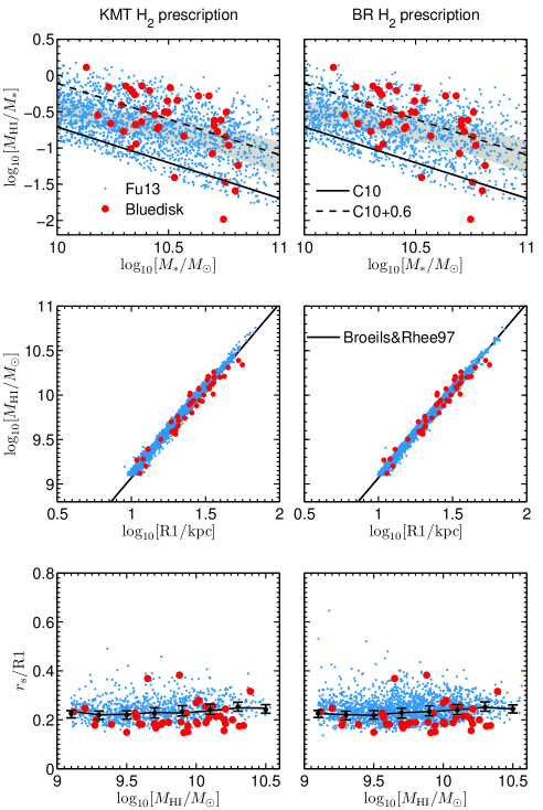
Figure 11: The comparison between the Fu13 model results and the Bluedisk observational sample. The two columns represent the Fu13 models with two H₂ fraction prescriptions (see Fu13 for details). In each panel, the blue dots represent the model sample and the red dots are for the Bluedisk sample. Top two panels: The HI-to-stellar mass ratio as a function of stellar mass. The gray areas represent the $\pm 1\sigma$ deviations around the mean values for the Fu13 model sample. For comparison, the black solid lines show the median relation in C10 and black dashed lines are offsets from solid lines by 0.6 dex. Middle two panels: The HI mass-size relation. The R1 values from observations are corrected for beam-smearing effects and R1 values from models are un-convolved. The black lines represent the fitting equation in Broeils & Rhee (1997, the diameter $D1$ is converted to radius R1). Bottom two panels: The relation between $r_{\rm s}/$R1 and HI mass. The black solid curves represent the model median values and the error bars represent the $\pm 1\sigma$ deviations around the median values for the model sample. $r_{\rm s}/$R1 values from models are un-convolved and $r_{\rm s}/$R1 values from Bluedisk observations are beam-corrected values.

In the top two panels of Fig. 11, we show the HI-to-stellar mass ratio as a function of stellar mass for the Fu13 model galaxies and the Bluedisk sample. The two panels represent the model results with two H₂ fraction prescriptions. The blue points correspond to individual model galaxies, while the red points correspond to individual Bluedisk galaxies. The grey shaded area shows the 1$\sigma$ deviation around the median relation between $M_{\rm HI}/M_{*}$ and $M_{*}$ for the model galaxies. By construction, the model galaxies span the same range in stellar mass and HI mass fraction as the Bluedisk sample. In the middle two panels of Fig. 11, we show the HI mass-size relation for the models and the data. The R1 values from the observations are corrected for beam-smearing and the model values are un-convolved. The model results fit both the Broeils & Rhee (1997) and the observational data extremely well. We will discuss the origin of the tight correlation between HI disk mass and size in the models in more detail in Section 6.2. Finally, the bottom two panels show the relation between $r_{\rm s}/$R1 and HI mass for both models and data. $r_{\rm s}$ is defined as the scale-length of the HI profile at $r>0.75$R1 obtained by fitting an exponential profile to this region of the disk. The black solid curves show the model median values and the error bars represent the $\pm 1\sigma$ deviations around the median. $r_{\rm s}/$R1 is around 0.22 to 0.24 for model galaxies, compared to 0.19 for the Bluedisk sample.

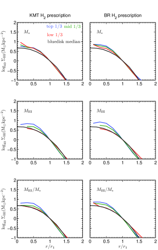
Figure 12: The relation between beam-convolved HI radial surface density profiles $\Sigma_{\rm HI}$ and the normalized radius $r/$R1 from the Fu13 model. The two columns represent the results of models with two H₂ fraction prescriptions. Similar to Fig. 4, the model samples are equally divided into 3 parts by $M_{*}$, $M_{\rm HI}$ and $M_{\rm HI}/M_{*}$ from the top to bottom rows. In each panel, the red, green and blue curves represent the median profiles in the lowest to highest parameter bins. The black curves represent the median curves from the whole Bluedisk sample.

Finally, in Fig. 12, we show the beam-convolved HI radial surface density profiles in units of $r/$R1 from the Fu13 models with two H₂ fraction prescriptions. Similar to Fig. 4, we divide model samples into 3 equal parts according to stellar mass $M_{*}$, HI mass $M_{\rm HI}$, and HI-to-stellar mass ratio $M_{\rm HI}/M_{*}$, from the top to bottom rows. In each panel, the red, green and blue curves represent the median model profiles for the highest,intermediate and lowest values of each parameter. The black curves show the median profile of the Bluedisk sample.

As can be seen, the model and the observational profiles agree extremely well in the outer disk. The HI density profiles in the inner disk are systematically too high compared to observations. When the sample is split according to HI mass or HI mass fraction, the same qualitative trends are seen in both models and data. We will explain the origin of these trends in the next section.

6 Interpretation of the results

6.1 Outer HI profiles in semi-analytic models

We have demonstrated that the outer disk HI surface density profiles have universal form when scaled to a radius corresponding to a fixed HI surface density and that the slope of the outer disk $r_{\rm s}/$R1 is almost constant among different galaxies.

In the Fu13 models, newly infalling gas is assumed to be distributed exponentially and is directly superposed onto the pre-existing gas profile from the previous time step. Gas also flows towards the centre of the disk with inflow velocity $v_{\rm inflow}=\alpha r$ ($v_{\rm inflow}\sim$ 7 km/s at a galactocentric radius of 10 kpc) . Following the prescription in Mo, Mao & White (1998), the scale length of the exponential infalling gas is given by $r_{\rm cool}=\left(\lambda/\sqrt{2}\right)r_{\rm vir}$, in which $\lambda$ and $r_{\rm vir}$ are the spin parameter and virial radius of the galaxy’s dark matter halo. Since the increase of $r_{\rm vir}$ and $r_{\rm cool}$ scales with the age of the Universe, the outer disk gas profiles are mainly determined by recent gas accretion. This disk galaxy growth paradigm is called “inside-out” disk formation (e.g Kauffmann et al. 1996; Dutton 2009; Fu et al. 2009), and an illustration of inside-out growth of the gas disk can be found in Fig. 1 in Fu et al. (2010).

According to the definition of outer disk scale-length $r_{\rm s}$, the outer disk HI surface density profile can be written as

$$\Sigma_{\rm{HI}}=\Sigma_{0}\exp\left(-\frac{r}{r_{\rm s}}\right)$$ (9)

in which $\Sigma_{0}$ is disk central HI surface density extrapolated from the outer disk HI profile. Let us suppose that $r_{\rm s}$ in Eq. (9) is approximately equal to $r_{\rm infall}$ at the present day, and $\Sigma_{0}$ represents the amount of gas accreted at $r=0$ in the recent epoch.

Substituting $1M_{\odot}\rm{pc^{-2}}=\Sigma_{0}\exp(-{\rm R1}/r_{\rm s})$ into Eq. (9), $r_{\rm s}/$R1 can be written as

$$\frac{{{r_{\rm{s}}}}}{{{{\rm R1}}}}=\frac{1}{{\ln\left[\Sigma_{0}/{M_{\odot}}{\rm{pc}}^{-2}\right]}}.$$ (10)

Eq. (10) implies that $r_{\rm s}/$R1 actually relates to the amount of recent gas accretion at $r=0$. For simplicity, we define $\dot{\Sigma}_{0}=d\Sigma_{0}/dt$ as the cold gas infalling rate at $r=0$.

We have tested the correlation between $r_{\rm s}/$R1 and $\dot{\Sigma}_{0}$ averaged over different timescales. We find the best correlation with $r_{\rm s}/R1$ if $\dot{\Sigma}_{0}$ is averaged over a timescale corresponding to the past 0.5 Gyr. In the left panel of Fig. 13, we plot the relation between $r_{\rm s}/R1$ and $1/\ln\dot{\Sigma}_{0}$ (averaged in the recent 0.5 Gyr) for model galaxies with $M_{*}>10^{10}M_{\odot}$ and $M_{\rm HI}>10^{9}M_{\odot}$, based on KMT H₂ prescription. The blue solid line represents the fitting equation

$$r_{\rm s}/{\rm R1}=0.065+\left(\ln\left[\dot{\Sigma}_{0}/M_{\odot}\rm{pc^{-2}Gyr^{-1}}\right]\right)^{-1}.$$ (11)

However, we note that a correlation between $r_{\rm s}/$R1 and HI excess ($\Delta\rm{f_{HI}}$) is not found from the observation (section 3.3).

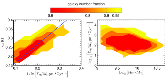
Figure 13: Left panel: the relation between $r_{\rm s}/$R1 and $1/\ln\left[\dot{\Sigma}_{0}/M_{\odot}\rm{pc^{-2}Gyr^{-1}}\right]$ for model galaxies. $\dot{\Sigma}_{0}$ is the gas infall rate in the disk centre averaged over the past 0.5 Gyr and $r_{\rm s}$ is the exponential scale length of the outer disk. The blue solid line is the fitting line Eq. (11). Right panel: the relation between $\dot{\Sigma}_{0}$ and $M_{\rm HI}$ for model galaxies. In both panels, the galaxies are from model results with KMT H₂ fraction prescription at $z=0$. The contours indicate the fraction of model galaxies located in a given region of parameter space, as given by the colour key at the top of the plot.

The right panel of Fig. 13 shows the relation between $M_{\rm HI}$ and $\dot{\Sigma}_{0}$. There is no relation between the two quanties, i.e. HI mass alone cannot be used to infer the recent accretion rate of a galaxy.

To summarize: the universal outer disk profiles in the semi-analytic models originate from the combination of the assumption that infalling gas has an exponential profile and of the inside-out growth of disks.

6.2 Inner HI profiles in semi-analytic models

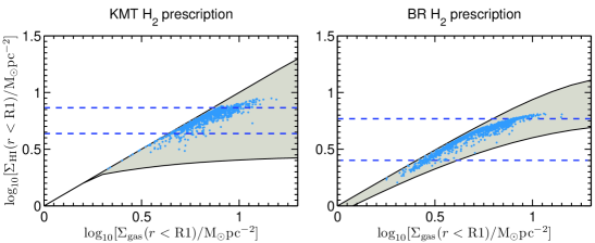
Figure 14: The relation between inner disk ($r<$R1) HI surface density and total cold gas surface density from Fu13 models. The blue dots in two panels are model samples with two $\rm{H_{2}}$ prescriptions. The two dashed lines in each panel indicate the values of $\Sigma_{\rm HI}(r<{\rm R1})$ that contain $90\%$ percent of the model samples. The gray areas represent the relations of $\Sigma_{\rm HI}$ vs. $\Sigma_{\rm gas}$ results directly calculated from the two $\rm{H_{2}}$-HI transition prescriptions in Fu13.

In the inner part ($r<$R1) of the disks, the HI surface density is mainly determined by the conversion between atomic and molecular gas. Higher total gas surface density ($\Sigma_{\rm{gas}}=\Sigma_{\rm{HI}}+\Sigma_{\rm{H_{2}}}$) leads to higher $\rm{H_{2}}$-to-HI ratio, which maintains the value of $\Sigma_{\rm{HI}}$ in a narrow range. In Fig. 14 , we plot HI surface density as a function of total cold gas surface density in the inner disks for model galaxies. We define $\Sigma_{\rm{HI}}(r<{\rm R1})=M_{\rm HI}(r<{\rm R1})/\pi{\rm R}{1^{2}}$ and $\Sigma_{\rm{gas}}(r<{\rm R1})=M_{\rm HI+\rm{H_{2}}}(r<{\rm R1})/\pi{\rm R}{1^{2}}$. We show results for two $\rm{H_{2}}$ fraction prescriptions. In each panel, the dashed lines indicate the values of $\Sigma_{\rm HI}(r<{\rm R1})$ that enclose 90% percent of the model galaxies . The gray areas indicate the region of the $\Sigma_{\rm gas}$ versus $\Sigma_{\rm HI}$ plane that is plausibly spanned by the two atomic-to-molecular gas transition prescriptions. For the KMT $\rm{H_{2}}$ prescription, we adopt a range in gas metallicity relative to the solar value $\rm{[Z/H]_{gas}}$ from -0.5 to 1. For the BR $\rm{H_{2}}$ prescription, we adopt a range in stellar surface density $\sqrt{\Sigma_{*}\Sigma^{0}_{*}}$ (see Equation 32 in Fu et al. 2010) from $1~{}M_{\odot}\rm{pc^{-2}}$ to $4000~{}M_{\odot}\rm{pc^{-2}}$. We note that in practice 90 % of the model galaxies have $\Sigma_{\rm HI}(r<{\rm R1})$ values between $\sim 3$ and $\sim 4M_{\odot}\rm{pc^{-2}}$.

To summarize: it is the combination of a narrow range in inner HI surface density and a “Universal” outer exponential profile that leads to the very tight HI mass-size relation. We note that the atomic-to-molecular gas conversion plays the more important role, because the inner disk contains a larger fraction of the total HI gas compared to the outer disk.

6.3 Main caveats

We note that the assumption that gas accreted from the halo is distributed on the disk with an exponential profile has no a priori physical justification. Bullock et al (2001) studied the angular momentum profiles of a statistical sample of halos drawn from high-resolution N-body simulations of the $\Lambda$CDM cosmology and showed that the cumulative mass distribution of specific angular momentum $j$ in halos could be fit with a function that follows a power law and then flattens at large $j$.

They explored implications of their M($<j$) profile on the formation of galactic disks assuming that $j$ is conserved during infall. They showed that the implied gas density profile deviates from an exponential disk, with higher densities at small radii and a tail extending to large radii.

It is thus something of mystery why the hydrodynamical simulations presented in this paper have outer disks that agree so well with the observed “universal” outer exponential profiles seen the data. The solution likely lies in the complicated interplay between the infall of new gas, star formation, supernova feedback and gas inflow processes occurring in the simulation and will form the subject of future work.

7 Summary

We have measured the azimuthally-averaged radial profiles of HI gas in 42 galaxies from the Bluedisk sample. We investigated how the shape of HI profiles vary as a function of galactic properties. We developed a model to describe the shape of HI profiles which is an exponential function of radius in the outer regions and has a depression towards the center. We derive maximum-likelihood estimates of $r_{\rm s}$, the scale radius of the outer exponential HI disk. By inverting the relation between star formation rate and $\rm{H_{2}}$ surface density, we also derive estimates of the total gas surface density profiles of our galaxies. Finally, we compare our observational results with predictions from SPH simulations and semi-analytic models of galaxy formation in a $\Lambda$CDM universe. The main results can be summarized as follows:

1. The HI disks of galaxies exhibit a homogeneous radial distribution of HI in their outer regions, when the radius is scaled to R1, the radius where the column density of the HI is 1$M_{\odot}$ pc^-2. The outer distribution of HI is well-fit by an exponential function with a scale-length of 0.18 R1. This function does not depend on stellar mass, stellar mass surface density, optical concentration index, global NUV-r colour, color gradient, HI mass, HI-to-stellar mass fraction, HI excess parameter, or HI disk morphologies.

2. By comparing the radial profiles of the HI-rich galaxies with those of the control systems, we deduce that in about half the galaxies, most of the excess gas lies outside the stellar disk, in the exponentially declining outer regions of the HI disk. In the other half, the excess is more centrally peaked.

3. The median total cold gas profile of the galaxies in our sample agrees well with the “universal” radial profile proposed by Bigiel & Blitz (2012). However, there is considerable scatter around the B12 parametrization, particularly in the outer regions of the disk.

4. Both the SPH simulations and Semi-analytical models are able to reproduce the homogeneous profile of HI in the outer region with the correct scale-length.

5. In the semi-analytic models, the universal shape of the outer HI radial profiles is a consequence of the assumption that infalling gas is always distributed exponentially. The conversion of atomic gas to molecular form explains the limited range of HI surface densities in the inner disk. These two factors produce the tight HI mass-size relation.

References

- Abazajian et al. (2009) Abazajian K. N. et al. 2009, ApJS, 182, 543
- Aumer et al. (2013) Aumer M., White S., Naab T., Scannapieco C., 2013, MNRAS, 434, 3142
- Bigiel et al. (2008) Bigiel F., Leroy A., Walter F., Brinks E., de Blok W. J. G., Madore B., Thornley M. D., 2008, AJ, 136, 2846
- Bigiel &Blitz (2012) Bigiel, F., Blitz, L., 2012, ApJ, 756, 183
- Blitz & Rosolowsky (2004) Blitz, L., & Rosolowsky, E. 2004, ApJ, 612, L29
- Blitz & Rosolowsky (2006) Blitz L., Rosolowsky E., 2006, ApJ, 650, 933
- Boylan-Kolchin et al. (2009) Boylan-Kolchin, M., Springel, V., White, S. D. M., Jenkins, A., & Lemson, G. 2009, MNRAS, 398, 1150
- Bosma (1978) Bosma, A., 1978, PhdT, 195B
- Broeils &Rhee (1997) Broeils, A. H., Rhee, M. -H., 1997, A&A, 324, 877
- Cayatte et al. (1990) Cayatte, V., van Gorkom, J. H., Balkowski, C., Kotanyi, C., 1990, AJ, 100, 604
- Catinella et al. (2010) Catinella, B., Schiminovich, D., Kauffmann, G., Fabello, S., Wang, J., 2010, MNRAS, 403, 683
- Conselice (2003) Conselice, C., 2003, ApJS, 147,1
- Chung et al. (2009) Chung, A., van Gorkom, J. H., Kenney, Jeffrey D. P., Crowl, H., Vollmer, B., 2009, AJ, 138, 1741
- Dutton et al. (2007) Dutton A. A., van den Bosch F. C., Dekel A., Courteau S., 2007, ApJ, 654, 27
- Elmegreen (1989) Elmegreen, B. G. 1989, ApJ, 338, 178
- Elmegreen (1993) Elmegreen B. G., 1993, ApJ, 411, 170
- Fu et al. (2009) Fu, J., Hou, J. L., Yin, J., & Chang, R. X. 2009, ApJ, 696, 668
- Fu et al. (2010) Fu J., Guo Q., Kauffmann G., Krumholz M. R., 2010, MNRAS, 409, 515
- Fu et al. (2013) Fu J., et al., 2013, MNRAS, 1755 (Fu13)
- Guo et al. (2011) Guo, Q., et al. 2011, MNRAS, 413, 101
- Jarrett et al. (2011) Jarret, T. H., Cohen, M., Masci, F., Wright, E., Stern, D., et al. 2011, ApJ, 735,112
- Jarrett et al. (2013) Jarret, T. H., Masci, F., Tsai, C. W., Petty, S. et al., 2013, AJ, 145, 6
- Kauffmann (1996) Kauffmann G., 1996, MNRAS, 281, 475
- Komatsu et al. (2011) Komatsu, E., et al. 2011, ApJS, 192, 18
- Krumholz et al. (2009) Krumholz, M. R., McKee, C. F., & Tumlinson, J. 2009, ApJ, 693, 216
- Leroy et al. (2008) Leroy A. K., Walter F., Brinks E., Bigiel F., de Blok W. J. G., Madore B., Thornley M. D., 2008, AJ, 136, 2782
- Lotz et al. (2004) Lotz, J. M., Primack, J., Madau, P., 2004, AJ, 613, 262
- Markwardt (2009) Markwardt, C. B. 2009, Astronomical Data Analysis Software and Systems XVIII, 411, 251
- Martin et al. (2010) Martin, A. M., Papastergis, E., Giovanelli R., Haynes M. P., Springob C. M., Stierwalt S., 2010, ApJ, 723, 1359
- Mo, Mao, & White (1998) Mo H. J., Mao S., White S. D. M., 1998, MNRAS, 295, 319
- Noordermeer et al. (2005) Noordermeer, E., van der Hulst, J. M., Sancisi, R., Swaters, R. A., van Albada, T. S., 2005, A&A, 442, 137
- Salim et al. (2007) Salim, S., Rich, R. M., Charlot, S., Brinchmann, J., et al. 2007, ApJS, 173, 267
- Springel et al. (2005) Springel V., et al., 2005, Natur, 435, 629
- Swaters et al. (2002) Swaters, R. A., van Albada, T. S., van der Hulst, J. M., Sancisi, R., 2002, A&A, 390, 829
- van der Hulst et al. (2001) van der Hulst, J. M.; van Albada, T. S.; Sancisi, R.,2001, ASPC, 240, 451V
- Verheijen & Sancisi (2001) Verheijen, M. A. W., Sancisi, R., 2001, A&A, 370, 765
- Wang et al. (2013) Wang, J., Kauffmann, G., Józsa, G. I. G., Serra, P., et al. 2013, MNRAS, 433, 270 (Paper I)
- Warmels (1988) Warmels, R. H., 1988, A&AS, 72, 19
- Weavers et al. (1984) Weavers, B. M. H. R., Appleton, P. N., Davies, R. D., Hart, L., 1984, A&A, 140, 125
- Wright et al. (2010) Wright, E., L, Eisenhardt, P. R. M., Mainzer, A. K., Ressler, M. E., et al. 2010, AJ, 140, 1868