A meta-analysis of the magnetic line broadening
in the solar atmosphere

A multi-line Bayesian analysis of the Zeeman broadening in the solar atmosphere is presented. A hierarchical probabilistic model, based on the simple but realistic Milne-Eddington approximation to the solution of the radiative transfer equation, is used to explain the data in the optical and near infrared. Our method makes use of the full line profiles of a more than 500 spectral lines from 4000 Å to 1.8 $\mu$m. Although the problem suffers from a strong degeneracy between the magnetic broadening and any other remaining broadening mechanism, the hierarchical model allows to isolate the magnetic contribution with reliability. We obtain the cumulative distribution function for the field strength and use it to put reliable upper limits to the unresolved magnetic field strength in the solar atmosphere. The field is below 160-180 G with 90% probability.

1 Introduction

The physical characteristics of the outer layers of the solar atmosphere are controlled by the magnetic field, because the magnetic pressure in the chromosphere and corona is larger than the gas pressure. Ultimately, the magnetic energy present in these outer layers is extracted from the energy stored in the photosphere. Consequently, it is of interest to have reliable estimations of the magnetic energy that is present in the photosphere.

Magnetic field diagnostics of the solar surface magnetism based on the polarization signals induced by the Zeeman effect are prone to cancellations if the magnetic field is organized at scales below the resolution element of the telescope. Despite this drawback, our understanding of the solar (photospheric) magnetism is fundamentally based on polarimetric studies of the Zeeman effect. Over the years, other tools that are less or not affected by cancellations have been devised. Among them, we can find the study of broadening mechanisms in spectral lines (Stenflo & Lindegren 1977) or the analysis of the Hanle effect in selected spectral lines (Stenflo 1982; Faurobert et al. 2001; Trujillo Bueno et al. 2004). It is well-known that the Zeeman signals in circular polarization depend on the projection of the magnetic field on the line-of-sight, while in linear polarization, they depend on the projections of the magnetic field on the plane of the sky. In the case of the Zeeman broadening and the Hanle effect in microturbulent fields, the effect on the spectral line depends fundamentally on the strength of the magnetic field. Therefore, no cancellation of the effect occurs even if the magnetic field is organized at scales below the resolution element. Both techniques have been used in the past to constrain the magnetic energy stored in the solar photosphere. Stenflo & Lindegren (1977) inferred, using the Zeeman broadening, an upper limit of 140 G for the rms magnetic field, which would correspond to a magnetic energy of $B^{2}/8\pi\sim 780$ erg cm^-3. Trujillo Bueno et al. (2004) obtained, using the Hanle effect in the Sr i line at 4607 Å in the microturbulent regime, an average magnetic field of 130 G if the intensity follows an exponential distribution. They also calculated that the intensity is 60 G if the field is homogeneous and volume-filling. This work was extended to a realistic three-dimensional magneto-convection simulation by Shchukina & Trujillo Bueno (2011). They found that the field distribution in the simulation has to be increased by a factor $\sim$10 in order to fit the observations. The ensuing magnetic energy is similar to that obtained by Trujillo Bueno et al. (2004) using ad-hoc distributions.

The main disadvantage of the Zeeman broadening to measure magnetic fields is that isolating the magnetic broadening from the remaining broadening mechanisms is extremely difficult and uncertain. This interplay has been recently analyzed in three-dimensional simulations of solar magneto-convection (Fabbian et al. 2010). In an effort to overcome the difficulties, Stenflo & Lindegren (1977) proposed to pursue a statistical approach, using Fourier Transform Spectrometer observations of many Fe i lines to infer an upper limit to the magnetic field in the solar atmosphere. The idea is based on the fact that, although the Zeeman broadening changes from line to line, it is proportional to a factor that depends on the quantum numbers and Landé factors of the levels involved in the transition. To exploit this property, Stenflo & Lindegren (1977) proposed a phenomenological formula to explain the measured broadening of the lines in terms of the strength of the line, excitation potential and magnetic field. Later, Solanki & Stenflo (1984, 1985) exploited the same phenomenological approach to study the magnetism of solar magnetic flux tubes, while Mathys & Stenflo (1986) and Mathys & Solanki (1989) extended this approach to other magnetic stars with success.

Our aim in this paper is to drop some of the previous simplifications present in the previous studies of the Zeeman broadening. First, instead of summarizing the width of the spectral line by a single number, we utilize the full spectral profile. Second, we use a simple but realistic line formation theory to generate the full line profile separating the Zeeman broadening from the remaining broadening mechanisms. Third, we analyze data in the near infrared, where the ratio between the Zeeman splitting and the Doppler broadening is larger. Finally, we use a hierarchical Bayesian model to put reliable constraints to the magnetic field.

2 Hierarchical modeling of line broadening

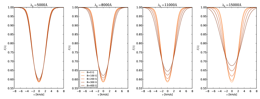
Figure 1: Line profiles emerging from a Milne-Eddington atmosphere with $\beta_{0}=2$, $\eta_{l}=3$ and $a=0.02$. The lines have a characteristic Doppler broadening of 2 km s^-1. Because the Doppler broadening is defined in velocity units, the broadening in wavelength units increases in proportion to the central wavelength of the line. We display the line profiles for five different microturbulent magnetic field strengths. We display the line profiles for five different microturbulent magnetic field strengths ($B=0,100,200,300,$ and $400$ G).

2.1 Observations

In this work we use observations from the optical and the near infrared part of the spectrum, both extracted from the National Solar Observatory (NSO) Fourier Transform Spectrometer (FTS). The observations in the optical have been obtained from Wallace et al. (1998), while the data for the near infrared has been extracted from Wallace & Livingston (2003). From the observed spectrum, we have isolated the spectral profiles of all the Fe i lines tabulated by Stenflo & Lindegren (1977) in the optical and from Ramsauer et al. (1995) in the near infrared. We built a specific graphical tool to inspect the FTS spectrum and decide which lines should be included in the study. The information from Stenflo & Lindegren (1977) and Ramsauer et al. (1995) is confronted with the spectroscopic information provided by the tabulation of Kurucz (1993) to find out if each individual line is isolated and free of blends. Lines with clear blends in one of the wings have been also accepted but removing the wavelengths of the blend. Heavy blended lines or those with very shallow profiles are discarded. For each line, the tool allows us to manually mark the wavelength span, which we select as that where the intensity reaches the continuum intensity. To avoid problems in the continuum, the intensity spectrum is re-normalized to the continuum for each line. Correlating the linelist of Stenflo & Lindegren (1977) and Ramsauer et al. (1995) with data tabulated by Kurucz (1993), we extract the central wavelength of the line, the total angular momenta and Landé factors of the upper and lower level of the transition. For almost all the tabulated lines, we can reliably find a line in the tabulation of Kurucz (1993) with all the atomic information. In any of the few cases in which this does not happen, we discard the line. The central wavelength of the line is re-computed to avoid introducing additional nuisance parameters in the model that we describe in the following. After all the filtering, we end up with 387 spectral lines (from the original set of 402) that span from 4365 Å to 6860 Å and 166 (from the original set of 352 associated to Fe i) in the range from 1 $\mu$m to 1.8 $\mu$m. The fundamental reason for the reduction in the number of lines was the presence of a clear blend and/or very shallow lines that we decide not to use.

2.2 Generative model and likelihood

Our aim is to extract information about the Zeeman broadening from a large set of spectral lines. To this end, the first ingredient that we need is a generative model, i.e., a way of linking our physical model with the observations. In our case, we assume that the observed spectral line at wavelength $\lambda_{i}$ is given by:

$$I^{\mathrm{obs}}(\lambda_{i})=I(\mbox{\boldmath$\theta$},\lambda_{i})+\epsilon_{i},$$ (1)

where $I(\mbox{\boldmath$\theta$},\lambda_{i})$ represents the synthetic spectral line described in the following, that depends on a set of parameters $\theta$. Additionally, we make the assumption that the model spectral line is perturbed with $\epsilon_{i}$, that represents noise, uncertainties and defects of our proposed model. If $\epsilon_{i}$ is just photon noise, it is safe to assume that it follows a Gaussian distribution with zero mean and variance $\sigma^{2}$. If we allow $\epsilon_{i}$ to absorb other systematic effects, this distribution becomes an approximation and one should potentially take into account the covariance between different wavelength points. This more complicated case is surely the one that we have with the FTS observations because the spectrum is obtained as an inverse Fourier transform of visibilities, which induces correlations that might be of importance. However, for the sake of simplicity and the lack of a reliable estimation for the covariance matrix, we assume that $\epsilon_{i}$ follows a Gaussian distribution with zero mean and variance $\sigma^{2}$.

In the following, we describe the simple but powerful model that we use to synthesize a spectral line in the presence of an isotropic and microturbulent magnetic field, i.e., we make explicit the functional form of $I(\mbox{\boldmath$\theta$},\lambda_{i})$ and the meaning of the vector of parameters $\theta$. Under the assumption of a sufficiently weak magnetic field and neglecting magneto-optical effects, the intensity emerging in a spectral line from a Milne-Eddington atmosphere can be written using the following simple approximate expression (e.g., Landi Degl’Innocenti & Landolfi 2004):

$$I(\lambda)=B_{0}\left[1+\frac{\beta_{0}\mu}{1+\eta_{l}\Psi(\lambda-\lambda^{\prime})}\right],$$ (2)

In the previous equation, $B_{0}$ and $\beta_{0}$ describe the variation of the source function with optical depth, so that $S=B_{0}+\beta_{0}\tau$. Additionally, $\mu=\cos\theta$ refers to the cosine of the heliocentric angle, $\eta_{l}$ is the ratio between the line opacity and the continuum opacity and $\lambda^{\prime}=\lambda_{0}(1+v/c)$ is the central wavelength of the transition under study ($\lambda_{0}$) shifted by the Doppler effect due to any bulk motion with velocity $v$. The line absorption profile is described using a Voigt profile:

$$\Psi(\lambda-\lambda_{0})=\frac{1}{\sqrt{\pi}}H\left(\frac{\lambda-\lambda^{\prime}}{\Delta\lambda_{D}},a\right),$$ (3)

where $\Delta\lambda_{D}=\lambda_{0}\Delta v_{D}/c$, with $c$ the speed of light, is the Doppler width in velocity units and $a$ is the damping coefficient.

Very far from the line center, where $\Psi(\lambda-\lambda^{\prime})=0$, the continuum intensity is given by $I_{c}=B_{0}(1+\beta_{0}\mu)$. Therefore, if we normalize the intensity spectrum by the continuum, we get

$$I(\mbox{\boldmath$\theta$},\lambda)=\frac{1}{1+\beta_{0}\mu}\left[1+\frac{\beta_{0}\mu}{1+\eta_{l}\Psi(\lambda-\lambda^{\prime})}\right].$$ (4)

It is then clear that the continuum normalized emergent intensity spectrum is independent of $B_{0}$.

When an isotropic, microturbulent and weak magnetic field is present in the line formation region, the model for radiative transfer is still valid if the line absorption profile is modified. If the three components of the magnetic field vector are characterized by a Gaussian distribution with zero mean and standard deviation $B$, the line profile that enters into Eq. (4) reads (Landi Degl’Innocenti & Landolfi 2004):

$$\Psi(\lambda-\lambda^{\prime})=\frac{\Delta\lambda_{D}}{\Delta\lambda_{T}}\frac{1}{\sqrt{\pi}}H\left(\frac{\lambda-\lambda^{\prime}}{\Delta\lambda_{T}},a\frac{\Delta\lambda_{D}}{\Delta\lambda_{T}}\right).$$ (5)

This expression is valid at second order in the Zeeman broadening ($\Delta\lambda_{B}^{T}$), defined as:

$$\Delta\lambda_{B}^{T}\sim 4.6686\times 10^{-13}\lambda_{0}^{2}B,$$ (6)

with $B$ given in G, and $\Delta\lambda_{B}^{T}$ and $\lambda_{0}$ in Å. We note that $\Delta\lambda_{B}^{T}\ll\Delta\lambda_{D}$ for the magnetic fields and temperatures expected in the quiet Sun. According to Landi Degl’Innocenti & Landolfi (2004), the broadening of the spectral line when a microturbulent field is present is a result of the quadratic sum of the Doppler broadening and the Zeeman broadening, so that

$$\Delta\lambda_{T}=\left[\Delta\lambda_{D}^{2}+4\bar{G}_{T}\left(\Delta\lambda_{B}^{T}\right)^{2}\right]^{1/2}.$$ (7)

The factor $\bar{G}_{T}$ is the second-order effective Landé factor for turbulent fields and has the following expressions in terms of the total angular momenta of the upper and lower levels and their corresponding Landé factors:

$$\bar{G}_{T}=\bar{g}^{2}+\frac{1}{16}g_{d}^{2}\left(4s-d^{2}-4\right),$$ (8)

with

$$s =J_{u}(J_{u}+1)+J_{l}(J_{l}+1)$$

$$d =J_{u}(J_{u}+1)-J_{l}(J_{l}+1)$$

$$g_{d} =g_{u}-g_{l}$$

$$g_{s} =g_{u}+g_{l}$$

$$\bar{g} =\frac{1}{2}g_{s}+\frac{1}{4}g_{d}d.$$ (9)

All the previous ingredients allow us to synthesize a spectral line emerging from a Milne-Eddington atmosphere with a microturbulent magnetic field using the vector of parameters $\mbox{\boldmath$\theta$}=(\beta_{0},\eta_{l},\Delta v_{D},a,B)$. Examples of the influence of a microturbulent magnetic field on the line profiles are shown in Fig. 1. Note that the influence of the Zeeman broadening increases with wavelength, so that it is important to focus on lines in the red part of the spectrum to constrain the influence of a magnetic field. It is conspicuous that the effect remains extremely subtle and can be easily confounded with any kind of non-magnetic broadening. This is the reason why a hierarchical probabilistic modeling is of help, as we show in this paper.

Once the generative model is proposed, it is straightforward to write down the likelihood, $\mathcal{L}$. This sampling distribution gives the probability of obtaining our current observations given that they have been generated with the model presented in the previous paragraphs. In our case, our generative model results in the following likelihood for a single spectral line $i$:

$$\mathcal{L}_{i}(D_{i}|\mbox{\boldmath$\theta$}_{i},\sigma_{i})=\prod_{j=1}^{{N_{\lambda}}_{i}}\frac{1}{\sqrt{2\pi}\sigma_{i}}\exp\left[-\frac{\left(I^{\mathrm{obs}}(\lambda_{j})-I(\mbox{\boldmath$\theta$}_{i},\lambda_{j})\right)^{2}}{2\sigma_{i}^{2}}\right],$$ (10)

a consequence of assuming that the intensity of different wavelengths are uncorrelated. Note that ${N_{\lambda}}_{i}$ is the number of wavelength points which are used to sample line $i$. We use the compact representation $D_{i}$ to refer to the intensity spectrum of a single line extracted from the FTS atlas. Likewise, we use $D=\{D_{1},D_{2},\ldots,D_{N}\}$ the full set of observations. Using the same line of reasoning, the total likelihood that takes into account all the lines is given by:

$$\mathcal{L}(D|\mbox{\boldmath$\theta$},\mbox{\boldmath$\sigma$})=\prod_{i=1}^{N}\mathcal{L}_{i}(D_{i}|\mbox{\boldmath$\theta$}_{i},\sigma_{i}),$$ (11)

where $\mbox{\boldmath$\theta$}=\{\mbox{\boldmath$\theta$}_{1},\mbox{\boldmath$\theta$}_{2},\ldots,\mbox{\boldmath$\theta$}_{N}\}$ and $\mbox{\boldmath$\sigma$}=\{\sigma_{1},\sigma_{2},\ldots,\sigma_{N}\}$.

2.3 Hierarchical model

Taking into account all the previous considerations, the probabilistic model used in this work is graphically represented in Fig. 2. The intensity spectrum of each line depends on the parameters $\beta_{0}$, $\eta_{l}$, $a$, $\Delta v_{D}$ and $B$. The synthetic profile, obtained applying Eq. (4), are then compared with the observed profiles extracted from the FTS atlas using an unknown noise standard deviation $\sigma$. This model is repeated for all the $N$ lines that we introduce in the analysis.

We are interested on the statistical properties of the magnetic field when the information encoded on all lines are simultaneously taken into account. To this end, we follow the standard way of Bayesian hierarchical models. It consists of using parametric priors (the parameters of the prior are termed hyperparameters) and making the inference hierarchical: the model parameters are the lowest level while the hyperparameters represent the upper level. The graphical representation of Fig. 2 gives a clear idea of the meaning of the hierarchical model. The magnetic field strength associated to each spectral line is assumed to be extracted from a common distribution (prior) that depends on the set of hyperparameters $\mathbf{x}_{B}$. This hierarchical scheme can be exploited to compute the distribution of a model parameter to which one has no direct observational access. In our case, we use a sufficiently general parametric prior distribution and the values of the hyperparameters are inferred from the data under the Bayesian framework. For convenience, we also use this hierarchical structure for the Doppler velocity, making the assumption that the Doppler widths are extracted from a common distribution.

Using the standard Bayesian approach, all the information about the model parameters is contained in the joint posterior $p(\mbox{\boldmath$\beta$}_{0},\mbox{\boldmath$\eta$}_{l},\Delta\mathbf{v}_{D},\mathbf{a},\mathbf{B},\mathbf{x}_{B},\mathbf{x}_{v}|D)$, which can be computed from the likelihood (defined above) and the prior distribution, $p(\mbox{\boldmath$\beta$}_{0},\mbox{\boldmath$\eta$}_{l},\Delta\mathbf{v}_{D},\mathbf{a},\mathbf{B},\mbox{\boldmath$\sigma$},\mathbf{x}_{B},\mathbf{x}_{v})$, using the Bayes theorem:

$$p(\mbox{\boldmath$\beta$}_{0},\mbox{\boldmath$\eta$}_{l},\Delta\mathbf{v}_{D},\mathbf{a}, \mathbf{B},\mbox{\boldmath$\sigma$},\mathbf{x}_{B},\mathbf{x}_{v}|D)\propto\mathcal{L}(D|\mbox{\boldmath$\beta$}_{0},\mbox{\boldmath$\eta$}_{l},\Delta\mathbf{v}_{D},\mathbf{B},\mathbf{a},\mbox{\boldmath$\sigma$},\mathbf{x}_{B},\mathbf{x}_{v})$$

$$\times p(\mbox{\boldmath$\beta$}_{0},\mbox{\boldmath$\eta$}_{l},\Delta\mathbf{v}_{D},\mathbf{a},\mathbf{B},\mbox{\boldmath$\sigma$},\mathbf{x}_{B},\mathbf{x}_{v}).$$ (12)

Using the conditional dependencies shown in Fig. 2, we can greatly simplify the likelihood and the prior distribution. The posterior for the hierarchical model becomes:

$$p(\mbox{\boldmath$\beta$}_{0},\mbox{\boldmath$\eta$}_{l}, \Delta\mathbf{v}_{D},\mathbf{a},\mathbf{B},\mbox{\boldmath$\sigma$},\mathbf{x}_{B},\mathbf{x}_{v}|D)\propto\mathcal{L}(D|\mbox{\boldmath$\beta$}_{0},\mbox{\boldmath$\eta$}_{l},\Delta\mathbf{v}_{D},\mathbf{B},\mathbf{a},\mbox{\boldmath$\sigma$})$$

$$\times p(\mbox{\boldmath$\beta$}_{0})p(\mbox{\boldmath$\eta$}_{l})p(\mathbf{a})p(\mbox{\boldmath$\sigma$})p(\mathbf{B}|\mathbf{x}_{B})p(\mathbf{x}_{B})p(\Delta\mathbf{v}_{D}|\mathbf{x}_{v})p(\mathbf{x}_{v}).$$ (13)

Since we are interested in the global statistical properties of the magnetic field, $\mbox{\boldmath$\beta$}_{0}$, $\mbox{\boldmath$\eta$}_{l}$, $\Delta\mathbf{v}_{D}$, $\mathbf{a}$, $\mathbf{B}$, and $\sigma$ can be considered as nuisance parameters that have to be integrated out from the posterior. Therefore, our final result is the following posterior distribution for the hyperparameters:

$$p(\mathbf{x}_{B}|D) \propto\int\mathrm{d}\mbox{\boldmath$\beta$}_{0}\,\mathrm{d}\mbox{\boldmath$\eta$}_{l}\,\mathrm{d}\Delta\mathbf{v}_{D}\,\mathrm{d}\mathbf{a}\,\mathrm{d}\mathbf{B}\,\mathrm{d}\mbox{\boldmath$\sigma$}\,\mathrm{d}\mathbf{x}_{v}\mathcal{L}(D|\mbox{\boldmath$\beta$}_{0},\mbox{\boldmath$\eta$}_{l},\Delta\mathbf{v}_{D},\mathbf{B},\mathbf{a},\mbox{\boldmath$\sigma$})$$

$$\times p(\mbox{\boldmath$\beta$}_{0})p(\mbox{\boldmath$\eta$}_{l})p(\Delta\mathbf{v}_{D})p(\mathbf{a})p(\mbox{\boldmath$\sigma$})p(\mathbf{B}|\mathbf{x}_{B})p(\Delta\mathbf{v}_{D}|\mathbf{x}_{v})p(\mathbf{x}_{v})p(\mathbf{x}_{B}).$$ (14)

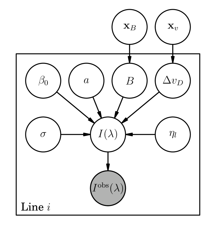
Figure 2: Graphical model representing the hierarchical Bayesian scheme that we used to analyze the broadening of spectral lines. Open circles represent random variables (note that both model parameters and observations are considered as random variables), while the grey circle represents a measured quantity. The frame labeled “Line $i$” represents that everything inside the frame has to be repeated for all the observations. An arrow between two nodes illustrates dependency. The nodes that are outside the frame are the hyperparameters of the model and are common to all pixels.

In words, our analysis proceeds as follows. We make the assumption that the shape of every line in the observations can be explained with a parametric Milne-Eddington model that depends on the gradient of the source function, the damping coefficient, the ratio of line and continuum opacities and the Doppler width of the line. To this Doppler width, we add quadratically the influence of an isotropic microturbulent magnetic field with a Gaussian distribution characterized by its standard deviation. We propose a sufficiently general parametric distribution for this standard deviation and we use all the lines to learn something about these parameters. We point out that, although there are large degeneracies in the model, we will be able to learn something about the distribution of magnetic fields thanks to the marginalization of the nuisance parameters.

2.4 Priors for parameters and hyperparameters

The prior distribution encodes all the a-priori information that we know about the parameters. In our case, we need to put priors over the parameters $\mbox{\boldmath$\beta$}_{0}$, $\mbox{\boldmath$\eta$}_{l}$, $\Delta\mathbf{v}_{D}$, $\mathbf{B}$, $\mathbf{a}$, and $\sigma$. The set of priors is summarized in Tab. 1, where we display the range of variation and the type of prior. A flat prior for variable $x$ in the interval $[a,b]$ is defined as $1/(b-a)$ if $a\leq x\leq b$ and zero elsewhere. The damping coefficient $a$, the ratio of line and continuum opacities $\eta_{l}$, and the Doppler width $\Delta\lambda_{D}$ have flat priors. The range of variation of each parameters is chosen based on previous experience fitting the line profiles. Given that $\beta_{0}$ and $\sigma$ can potentially span over several orders of magnitude, we choose a modified Jeffreys’ prior for them (Gregory 2005):

$$\mathrm{MJ}(x;x_{0},x_{\mathrm{max}})=\left[\left(x+x_{0}\right)\ln\left(\frac{x_{0}+x_{\mathrm{max}}}{x_{0}}\right)\right]^{-1}.$$ (15)

This prior behaves as a Jeffreys’ prior (i.e., as $x^{-1}$) for $x\gg x_{0}$ and as a uniform prior for $x\ll x_{0}$. The value of $x_{0}$ is chosen to be that of the lower limit, while $x_{\mathrm{max}}$ is selected to be the upper limit.

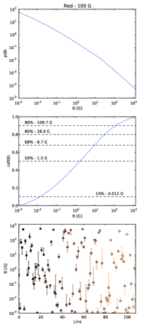
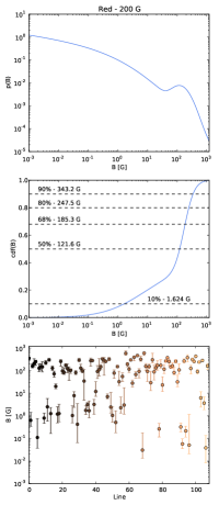
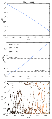
Figure 3: Distribution of magnetic fields inferred from the synthetic cases. The upper panels display the inferred probability density function. The middle panels show the corresponding cumulative distribution, where we have indicated the 10, 50, 68, 80, and 90% percentiles. Finally, the lower panels display a summary of the marginal posteriors for the field strength associated with each spectral line. Each line has a different color in a sequence to improve the readability of the figure.

Concerning the selection of the hierarchical prior distribution, it is important that the functional form is able to capture the full potential variability of the parameter. Even with a simple prior distribution, if we allow the hyperparameters to be random variables, a wide range of quite complex distributions can be achieved. Additionally, a desirable property of the hierarchical prior is that it is naturally defined in the range of the parameter of interest. A broad range of possibilities are available but we use previous successful experience (Asensio Ramos & Arregui 2013) and use simple prior distributions. After some initial experiments, we use a mixture of two log-normal prior distributions for $B$, truncated in the interval $[B_{\mathrm{min}},B_{\mathrm{max}}]$ (see Tab. 1 for the selected values of the limits):

$$p(B_{i}|\mathbf{x}_{B})=\left\{\begin{array}[]{clc}p\mathrm{LN}(B_{i};\mu_{B1},\gamma_{B1})&&B_{\mathrm{min}}\leq B\leq B_{\mathrm{max}}\\ +(1-p)\mathrm{LN}(B_{i};\mu_{B1},\gamma_{B2})&&\\ 0&&\mathrm{otherwise}\end{array}\right.$$ (16)

where a log-normal is defined as

$$\mathrm{LN}(B_{i};\mu,\gamma)=\frac{1}{\sqrt{2\pi}\gamma B_{i}}\exp\left[-\frac{(\log B_{i}-\mu)^{2}}{2\gamma^{2}}\right],$$ (17)

where $\mu$ and $\gamma$ are the hyperparameters, which fulfill $\gamma>0$, $-\infty<\mu<\infty$. Additionally, we have $0\leq p\leq 1$. In the notation used in Fig. 2, we have that $\mathbf{x}_{B}=(\mu,\gamma)$. One of the main properties of this prior is that, independently of the value of $\mu$ and $\gamma$, the probability of having $B=0$ tends to zero. This is in accordance with the fact that it is extremely improbable that the three components of an isotropic vector field become zero simultaneously (Domínguez Cerdeña et al. 2006; Sánchez Almeida 2007). The reason for using a mixture of two log-normals is that, in the synthetic cases displayed in Sec. 3.1, we find multimodal distributions for the field strength. This multimodality is a consequence of the fact that some lines are able to measure the presence of a magnetic field, while others are quite unsensitive. Therefore, the prior has to be flexible enough to capture this behavior.

Finally, a single log-normal is used as prior for $\Delta v_{D}$, as indicated in Tab. 1. The priors for the hyperparameters and the remaining parameters are shown in the same table. The range of parameters is chosen after running several experiments but they can be considered to be quite “uninformative”.

2.5 Sampling the posterior

For the analysis of $N=387$ lines in the optical, the posterior becomes a distribution in $6N+6=2328$ dimensions, while it goes down to 1003 dimensions for the $N=166$ lines in the near infrared. Obviously, to carry out the marginalization integrals required by Eq. (14) we need to rely on standard Markov Chain Monte Carlo (MCMC) schemes (e.g., Metropolis et al. 1953) or any other alternative. The dimensionality of our problem is so large that standard MCMC methods are not efficient and we resort to the Hamiltonian Monte Carlo (HMC) method Duane et al. (1987); Neal (2010), using the code of Lentati et al. (2013). These methods efficiently sample the posterior distribution by utilizing information not only of the log-posterior but also of its gradient. As a consequence, the sampling can make very long jumps in the space of parameters but keeping a high acceptance rate. The main drawback is that the computation of the gradient of the log-posterior can be cumbersome. In our case, a direct application of the chain rule allows us to compute the gradient of the log-posterior quite efficiently. Another drawback is that HMC methods are somehow dependent on the value of some internal parameters, that need to be adapted accordingly. We do this by an extensive initial study in which we tweak these parameters until we get a good acceptance rate. Finally, we use a sigmoid change of variables to improve the sampling efficiency, while avoiding sampling outside the prior ranges. For instance, for a parameter $x$ defined in the interval $[a,b]$, we transform it into $x^{\prime}$ using

$$x^{\prime}=\log\left(\frac{a-x}{x-b}\right),$$ (18)

Table 1: Priors

Parameter	Lower limit	Upper limit	Type
$\beta_{0}$	0.1	50	Mod. Jeffreys
$a$	0.01	0.6	Mod. Jeffreys
$\eta_{l}$	0	20	Flat
$\Delta v_{D}$ [km s-1]	0.2	6	Log-normal
$\sigma$	$10^{-4}$	0.1	Mod. Jeffreys
$B$ [G]	10-3	1200	Log-normal mixt.
$\mu_{v}$ [km s-1]	0.01	10	Flat
$\gamma_{v}$ [km s-1]	0.01	20	Mod. Jeffreys
$\mu_{B1}$ [G]	0.1	20	Flat
$\gamma_{B1}$ [G]	0.2	20	Mod. Jeffreys
$\mu_{B2}$ [G]	0.1	10	Flat
$\gamma_{B2}$ [G]	0.05	10	Mod. Jeffreys
$p$	0	1	Flat

which is then defined in $(-\infty,\infty)$ and no boundaries are needed. The derivatives of this transformation have to be taken into account on the derivatives of the log-posterior with respect to the model parameters in the HMC sampling.

Figure 4: Observed spectral lines in the optical (dots), together with the MAP fit (blue curve). The selected spectral lines are ordered by wavelength. The abscissa axis refer to the sampling of the FTS atlas. Note that the MAP fit does a very good job, demonstrating that the simplified Milne-Eddington model that we propose to explain the observations is quite accurate.

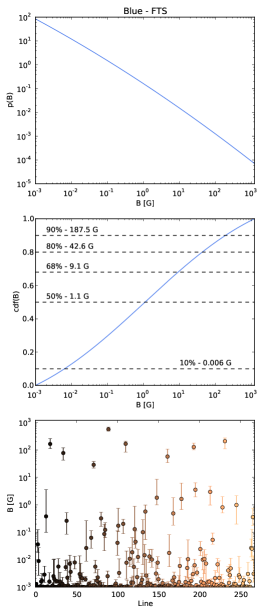
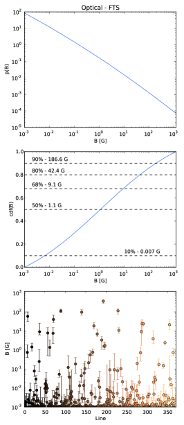
Figure 5: Like Fig. 3 but for the FTS atlas in the optical. For comparison, the left column displays the results for all lines below 6000 Å, the central column shows results for lines above 6000 Å, while the right column takes all lines into account. The results show that the field is below 186 G with 90% probability.

3 Results

3.1 Synthetic cases

The effect of a magnetic field on the broadening of a spectral line is very small and it is heavily degenerated with other broadening mechanisms. Therefore, it is interesting to test our complex probabilistic model with a synthetic case in which we know the input magnetic field strength. To this end, we synthesize the 387 spectral lines using the same Milne-Eddington model that we use to interpret it and add some noise. The line parameters are chosen uniformly randomly from the following intervals: $\beta_{0}\in[0.5,20]$, $\eta_{l}\in[0.5,20]$, $a\in[0,0.5]$, $\Delta v_{D}\in[0.5,2]$ km s^-1. The magnetic field is fixed at two values, 100 G and 200 G, and we also divide the spectral lines in two groups: lines in the blue part of the spectrum with $\lambda_{0}<6000$ Å and lines in the red part, with $\lambda_{0}>6000$ Å. Fig. 3 display the inferred distributions for all the cases. The first row shows the probability density function (pdf) obtained as the Monte Carlo average over the hyperparameters of the proposed prior distribution:

$$\langle p(B)\rangle=\frac{1}{N_{s}}\sum_{i=1}^{N_{s}}p_{i}\mathrm{LN}(B;\mu_{B1}^{i},\gamma_{B1}^{i})+(1-p_{i})\mathrm{LN}(B;\mu_{B1}^{i},\gamma_{B2}^{i}),$$ (19)

where $N_{s}$ is the number of samples obtained. The second row displays the ensuing cumulative distribution, numerically computed from the pdf. The last row shows a summary of the inferred values of the magnetic field associated to each line. Each point marks the median value of the marginal posterior, while the error bars indicate the $\pm 1\sigma$ confidence intervals. The two left columns refer to the cases using the red part of the spectrum, while the two right columns use the lines in the blue part. It is clear from these results that the lines in the blue are not able to put strong constraints on the magnetic field strength, even though the number of lines in the red part is much smaller. The data in the blue is able to say that the field is below $\sim$250 G with 90% probability and below $\sim 60-70$ G with 68% probability, not giving a clear hint that the two cases have different field strengths. As shown in the upper panels, the pdf is fundamentally dominated by one of the log-normals (we find $p\sim 1$), so we do not detect any hint of multi-modality. Additionally, the field inferred from many spectral lines hit the lower boundary of 10^-3 G that we impose with the prior, giving the idea that even weaker files would be preferred.

On the contrary, the constraints obtained from the red part of the spectrum are much more restrictive. For the case with 200 G, the data indicates that the field is below 343 G with 90% probability, while for the case with 100 G, this number goes down to 109 G. The pdf for the case with 200 G gives a clear hint for the presence of a bump around $\sim 200$ G. This bump produces that the percentile 50% and 68% give very similar magnetic fields (121 G and 185 G, respectively). This experiment demonstrates that our probabilistic model is able to extract information from the observations, in spite of the complexity and degeneracy of the problem.

3.2 Analysis of the FTS atlas in the optical

After the demonstration with synthetic data, we apply the very same probabilistic model to the observed FTS atlas. Even though we have tried to isolate the clean spectral lines, the simplified Milne-Eddington model is surely now less appropriate than in the synthetic model to explain the spectral lines. The presence of asymmetries and/or blends may affect our model, but they should be largely absorbed by the random variable $\sigma$. Lines where the Milne-Eddington model is not accurate will have an enhanced value of $\sigma$. In other words, the Bayesian model automatically detects that the information encoded in this line to constrain the model parameters is of less quality. Consequently, the relevance of these lines on the final conclusions will be decreased.

After sampling from the posterior, we locate the combination of model parameters giving the largest posterior, i.e., the maximum a-posteriori (MAP) solution. The spectrum resulting from this combination of parameters is displayed in Fig. 4. The observed spectral lines are shown in grey dots, while the best fit is shown in with the blue curve. We only display the fitted lines for the optical. The results in the near infrared are of the same quality. For convenience, the abscissa does not refer to real wavelength but to wavelength step. Given the specificities of the FTS atlas, the wavelength step for the lines in the blue is smaller than in the red. Figure 4 shows that the generative model proposed in this work does a good job on capturing the fundamental shape of the spectral lines. The residuals are small except in a reduced number of spectral lines.

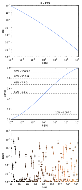
Figure 6: Like Fig. 3 but for the FTS atlas in the near infrared. The results in the optical and near infrared display a good consistency, with the data in the infrared yielding fields below 160 G with 90% probability.

Having shown the quality of the generative model, we analyze now the results from the hierarchical model. One of the main results of this paper is displayed in Figure 5. Like in the synthetic cases, we carry out the inference separately for lines below 6000 Å (blue) and above 6000 Å (red), but we also carry out the Bayesian inference for the whole set of spectra lines. Using the samples from the marginal distribution for $\mu_{B1}$, $\gamma_{B1}$, $\mu_{B2}$, $\gamma_{B2}$ and $p$, we compute the Monte Carlo approximation to the distribution of magnetic fields obtained from Eq. (19). The corresponding cumulative distribution function is shown in the middle panels of the figure, where we have marked a few quantiles of interest. The first thing to note is that the results are quite consistent independent of the spectral range used or if we use the full set of spectral lines. Second, the probabilistic analysis demonstrates that the the field is, with 90% probability, below $\sim 186$ G, although the upper limit remains hardly determined and hits the prior limit of 1200 G. The main reason for this is that there is a degeneracy on the line broadening mechanisms, so that if the Doppler broadening is very small, it is still possible to fit the spectral lines using magnetic broadening. Obviously, this possibility is limited by the presence of the upper limit to the magnetic field set by the prior. Finally, the analysis suggests that the majority of the spectral lines point to a very small magnetic field that hits the lower limit of the prior. However, the influence of the specific value of the lower limit of the prior is of reduced importance on the general results indicated by the cumulative distribution function. Only a few lines are the ones pushing the prior to higher magnetic fields.

3.3 Analysis of the FTS atlas in the near infrared

It is clear from Eq. (7) that, for a fixed magnetic field, the Zeeman broadening is larger in the red than in the blue. In spite of its great interest, investigating the Zeeman broadening in the infrared has been tackled only a few times. Trujillo Bueno et al. (2006) used synthesis in three-dimensional simulations of the solar atmosphere with ad-hoc turbulent magnetic fields in the Fe i lines at 15648 Å and 15652 Å. They pointed out that the Zeeman broadening can be potentially used in conjunction with other techniques to put constraints to the unresolved magnetic field. Later, Asensio Ramos et al. (2007) and Asensio Ramos (2009) analyzed observed and synthetic Stokes $I$ profiles of the Mn i line at 15262.7 Å to diagnose the magnetic field strength taking advantage of the strong Paschen-Back perturbations produced by the hyperfine structure. They concluded that the mean magnetic field has to be smaller than 250 G and organized at horizontal scales of $\sim$0.4”.

In this work, we apply a multiline technique to lines in the near infrared in order to put constraints to the non-resolved magnetic field in the solar photosphere. To this end, we applied the probabilistic model to the 166 lines that we isolated from the FTS atlas, and the results are displayed in Fig. 6. The cumulative distribution function points to fields below 160 G with 90% probability, and below 35 G with 80% probability.

4 Conclusions

We have used a probabilistic model of the formation of spectral lines in a Milne-Eddington atmosphere with a turbulent magnetic field with Maxwellian distribution to obtain the statistical properties of the average magnetic field from the FTS atlas of the solar spectrum. The difficulty of this approach deals on the reduced effect that a magnetic field has on the line broadening, together with the large degeneracy that the magnetic broadening has with other broadening mechanisms. In spite of this, our hierarchical model is able to extract this hidden information and we provide strong constraints to the turbulent magnetic field.

The difficulty of estimating the magnetic field is reflected on the long tails that the cumulative distribution functions have for strong fields. Even though the median value is 1 G for both the data in the optical and near infrared (the field is below 1 G with 50% probability), the field is smaller than 186 G with 90% probability from the optical data and below 160 G with 90% probability for the data in the near infrared. These results are not far from the original results of Stenflo & Lindegren (1977), who obtained a value of 140 G using the same spectral lines. Additionally, computing the magnetic energy associated to our estimated priors, we obtain $B^{2}/8\pi\sim 1430$ erg cm^-1 from the data in the optical and $\sim 1260$ erg cm^-1 from the near infrared data. These values are similar to those estimated by Trujillo Bueno et al. (2004) using the Hanle effect in the Sr i line at 4607 Å.

However, our statistical analysis departs from the study of Stenflo & Lindegren (1977) in a few important details. First, we make use of the full line profile and also from data in the near infrared. We simultaneously use information from the width of the line at all depths, contrarily to the analysis of Stenflo & Lindegren (1977) that was carried out for the width of the lines at a few discrete number of depths. Second, given our Bayesian approach to the probabilistic model, the results are given in terms of probability distributions, from where confidence intervals can be easily obtained. This is of special relevance in our problem, in which the desired piece of information is deeply degenerate and hidden. It is then important to give reliable confidence intervals. Finally, our results are given after marginalizing all the parameters except the magnetic field. Therefore, the confidence intervals that we extract from Fig. 5 already take into account our ignorance on the remaining model parameters.

The magnetic field included in our model should not be strictly interpreted as microturbulent. The FTS is an instrument with no spatial resolution inside a very large field of view, that can reach 40”. Therefore, the resulting intensity profile for each line is the result of the addition of many profiles, each one characterized by a magnetic field. Our assumption of a magnetic field strength with a Maxwellian distribution should then be understood as the global distribution of field strengths in the unresolved field-of-view.