The Hubbard model beyond the two-pole approximation:
a Composite Operator Method study

Abstract

Within the framework of the Composite Operator Method, a three-pole solution for the two-dimensional Hubbard model is presented and analyzed in detail. In addition to the two Hubbard operators, the operatorial basis comprises a third operator describing electronic transitions dressed by nearest-neighbor spin fluctuations. These latter, compared to charge and pair fluctuations, are assumed to be preeminent in the region of model-parameter space - small doping, low temperature and large on-site Coulomb repulsion - where one expects strong electronic correlations to dominate the physics of the system. This assumption and the consequent choice for the basic field, as well as the whole analytical approximation framework, have been validated through a comprehensive comparison with data for local and single-particle properties obtained by different numerical methods on varying all model parameters. The results systematically agree, both quantitatively and qualitatively, up to coincide in many cases. Many relevant features of the model, reflected by the numerical data, are exactly caught by the proposed solution and, in particular, the crossover between weak and intermediate-strong correlations as well as the shape of the occupied portion of the dispersion. A comprehensive comparison with other $n$-pole solutions is also reported in order to explore and possibly understand the reasons of such good performance.

I Introduction

Although the number of different trials to solve more or less exactly the two-dimensional Hubbard model Hubbard (1963) are countless and increase steadily since its advent in middle 50s, to time no analytical approximation method can be considered to have given a clear and definitive answer to the very many relevant issues raised by this very simple model. This latter contains only two terms, kinetic energy and local Coulomb repulsion, that can be cast in diagonal form in the two quantum-complementary direct and momentum spaces. This intrinsic incompatibility leads to many unexpected and very complex features still not all known or fully explored, and even less deeply understood. Together with the more fundamental and theoretical interest in this model, which is universally considered the prototypical model for strongly correlated systems, its relevance to real materials made the Hubbard model known in the whole solid state community and well beyond this latter. In particular, the model has been widely used to describe the archetypical Mott-Hubbard insulator $V_{2}O_{3}$ Imada et al. (1998) and the cuprate high-$T_{c}$ superconductors Bednorz and Müller (1986); Anderson (1987). The microscopic description of the anomalous behaviors experimentally observed in the cuprates, mainly in the underdoped region, in almost all experimentally measurable physical properties Alloul et al. (1989); Timusk and Statt (1999); Basov et al. (1999); Orenstein and Millis (2000); Damascelli et al. (2003); Shen et al. (2005); Eschrig (2006); Kanigel et al. (2006); Lee et al. (2006); Valla et al. (2006); Doiron-Leyraud et al. (2007); LeBoeuf et al. (2007); Bangura et al. (2008); Hossain et al. (2008); Yelland et al. (2008); Sebastian et al. (2008); Audouard et al. (2009); Meng et al. (2009); Anzai et al. (2010); Singleton et al. (2010); Sebastian et al. (2010a, b, c); Tranquada et al. (2010); Vishik et al. (2010); King et al. (2011); Laliberte et al. (2011); Ramshaw et al. (2011); Riggs et al. (2011); Sebastian et al. (2011a, b, c); Vignolle et al. (2011); Sebastian et al. (2012a, b) is still an open problem. Features not predicted by standard many-body theory and in contradiction with the Fermi-liquid framework and diagrammatic expansions, such as non-Fermi-liquid response, quantum criticality, pseudogap formation, ill-defined Fermi surface, kinks in the electronic dispersion, $\ldots$ , remain still unexplained or at least controversially debated Lee et al. (2006); Tremblay et al. (2006); Sebastian et al. (2012b). The Hubbard model is thought to contain by construction many of the key ingredients necessary to explain these anomalous features: strong electronic correlations, competition between localization and itinerancy, Mott physics, and low-energy spin excitations.

Numerical approaches Avella and Mancini (2013) are fundamental for benchmarking and fine tuning analytical theories and for establishing which are those capable to deal with the quite complex phenomenology of the Hubbard model. Unfortunately, numerical techniques cannot explore, because of their limited resolution in frequency and momentum, the most relevant regime of model parameters (small doping, low temperature and large on-site Coulomb repulsion) where one expects strong electronic correlations to dominate the physics of the system. As regards analytical and semi-analytical (i.e. embedding a numerical core) theories Avella and Mancini (2012a), a few are definitely worth mentioning: the work of Mori Mori (1965), Hubbard Hubbard (1963, 1964a, 1964b), Rowe Rowe (1968), Roth Roth (1969), Tserkovnikov Tserkovnikov (1981a, b), the Gutzwiller approximation Gutzwiller (1963, 1964, 1965); Brinkman and Rice (1970); Yokoyama and Shiba (1987); Gulácsi et al. (1993); Bünemann and Weber (1997); Dzierzawa et al. (1997); Bünemann et al. (1998); Seibold et al. (2003); Attaccalite and Fabrizio (2003); Ferrero et al. (2005); Capello et al. (2005); Fabrizio (2007); Lanatà et al. (2008); Ho et al. (2008); Deng et al. (2009); Schiró and Fabrizio (2010); Tocchio et al. (2011); Lanatà et al. (2012), the slave boson method Barnes (1976); Coleman (1984); Kotliar and Ruckenstein (1986), the spectral density approach Kalashnikov and Fradkin (1969); Nolting (1972), the two-particle self-consistent approach Tremblay et al. (2006), the RPA and equations-of-motion based techniques Chubukov and Norman (2004); Prelovšek and Ramšak (2005); Plakida and Oudovenko (2007), the dynamical mean-field theory (DMFT) Metzner and Vollhardt (1989); Georges and Kotliar (1992); Georges et al. (1996), the DMFT$+\Sigma$ approach Sadovskii et al. (2005); Kuchinskii et al. (2005, 2006) as well as all cluster-DMFT-like theoriesMaier et al. (2005) (the cellular-DMFT Kotliar et al. (2001), the dynamical cluster approximation Hettler et al. (1998) and the cluster perturbation theory Sénéchal et al. (2000)).

We have also been developing a systematic approach, the composite operator method (COM) The ; Avella and Mancini (2012b), to study highly correlated systems. In the last fifteen years, COM has been applied to several models and materials: Hubbard Hub ; Odashima et al. (2005), $p$-$d$ p-d , $t$-$t^{\prime}$-$U$ ttU , extended Hubbard ($t$-$U$-$V$) tUV , Kondo Villani et al. (2000), Anderson And , two-orbital Hubbard Plekhanov et al. (2011), Ising Isi , $J_{1}-J_{2}$ Avella et al. (2008); J1J , Cuprates Cup ; Avella and Mancini (2007a, b, 2008, 2009), etc The Composite Operator Method (COM) The ; Avella and Mancini (2012b) has the advantage to be completely microscopic, exclusively analytical, and fully self-consistent. COM recipe uses two main ingredients The ; Avella and Mancini (2012b): composite operators and algebra constraints. Composite operators are products of electronic operators and describe the new elementary excitations appearing in the system owing to strong correlations. According to the system under analysis The ; Avella and Mancini (2012b), one has to choose a set of composite operators as operatorial basis and rewrite the electronic operators and the electronic Green’s function in terms of this basis. Algebra Constraints are relations among correlation functions dictated by the non-canonical operatorial algebra closed by the chosen operatorial basis The ; Avella and Mancini (2012b). Other ways to obtain algebra constraints rely on the symmetries enjoined by the Hamiltonian under study, the Ward-Takahashi identities, the hydrodynamics, etc The ; Avella and Mancini (2012b). Algebra Constraints are used to compute unknown correlation functions appearing in the calculations. Interactions among the elements of the chosen operatorial basis are described by the residual self-energy, that is, the propagator of the residual term of the current after this latter has been projected on the chosen operatorial basis The ; Avella and Mancini (2012b). According to the physical properties under analysis and the range of temperatures, dopings, and interactions you want to explore, one has to choose an approximation to compute the residual self-energy. In the last years, we have been using the $n-$pole Approximation Hub ; Odashima et al. (2005); p-d ; ttU ; tUV ; Plekhanov et al. (2011); Isi ; Cup , the Asymptotic Field Approach Villani et al. (2000); And and the Non-Crossing Approximation (NCA) Avella and Mancini (2007a, b, 2008, 2009).

In this manuscript, we present an original three-pole approximate solution for the 2D single-band Hubbard model based on the COM. The not-standard choice of the third field in the operatorial basis, in addition to the two Hubbard operators, is justified in detail and validated a posteriori by the analysis of the correlations developing in the system. The quite involved self-consistency scheme is built step by step and the rationale behind each assumption is given and commented at length. The results of the proposed overall approximation scheme are successfully compared with both numerical simulations and other $n$-pole approximations so to fully characterize the solution and individuate strengths, weaknesses and their sources/causes. The main characteristics and relevant features of the proposed solutions are summarized as well as future possible improvements are discussed. The detailed plan of the paper follows.

In Sec. II, we discuss the model and the proposed approximation method. In particular, in Sec. II.1, we present the Hubbard Hamiltonian and part of the notation we will be using all over the manuscript. In Sec. II.2, we motivate the choice of the operatorial basis and give the corresponding equations of motion. In Sec. II.3, we discuss the projection of the currents on the chosen basis and introduce the polar approximation. In Sec. II.4, we derive a closed expression for the electronic Green’s function of the system and analyze the main relations to the relevant correlation functions. In Sec. II.5, we discuss the normalization matrix of the system and its entries. In Sec. II.6, we report the expression of the $m$-matrix and analyze its properties. In Sec. II.7, we discuss in detail the self-consistency scheme at the basis of the proposed approximation method and the Algebra Constraints characterizing it. In Sec. III, we present the results of the proposed approximation scheme. In particular, in Sec. III.1, we compare the three-pole approximation presented in the manuscript with other $n$-pole approximations. In Sec. III.2, we report a comprehensive comparison with different numerical methods for many local properties on varying all model parameters. In Sec. III.3, we discuss the bands and their single and double occupancy in order to deeper characterize the proposed approximation scheme. In Sec. III.4, we report spin, charge and pair correlation functions and analyze their behavior as function of filling and on-site Coulomb repulsion. Finally, in Sec. IV, we draw the conclusions and present a possible outlook. In App. A, we describe in detail the operatorial-projection scheme used to get correlation functions of fields not belonging to the chosen operatorial basis.

II Model and Methods

II.1 Hamiltonian

The Hamiltonian of the original (single-band, nearest-neighbor-hopping, on-site-Coulomb-repulsion) two-dimensional Hubbard model reads as

$$H=-4t\sum_{\mathbf{i}}c^{\dagger}\left(i\right)\cdot c^{\alpha}\left(i\right)+U\sum_{\mathbf{i}}n_{\uparrow}\left(i\right)n_{\downarrow}\left(i\right)-\mu\sum_{\mathbf{i}}n\left(i\right)$$ (1)

where

$$c\left(i\right)=\begin{pmatrix}c_{\uparrow}\left(i\right)\\ c_{\downarrow}\left(i\right)\end{pmatrix}$$ (2)

is the electronic field operator in spinorial notation and Heisenberg picture ($i=\left(\mathbf{i},t_{i}\right)$). $\cdot$ and $\otimes$ stand for the inner (scalar) and the outer products, respectively, in spin space. Hereafter, all composite fermionic-like operators (i.e. composed of an odd number of original electronic operators) are written in spinorial notation, as well as all composite bosonic-like operators (i.e. composed of an even number of original electronic operators) are scalars in the same notation. $\mathbf{i}=\mathbf{R_{i}}=\left(i_{x},i_{y}\right)$ is a vector of the two-dimensional square Bravais lattice, $n_{\sigma}\left(i\right)=c_{\sigma}^{\dagger}\left(i\right)c_{\sigma}\left(i\right)$ is the particle density operator for spin $\sigma$ at site $\mathbf{i}$, $n\left(i\right)=\sum_{\sigma}n_{\sigma}\left(i\right)=c^{\dagger}\left(i\right)\cdot c\left(i\right)$ is the total particle density operator at site $\mathbf{i}$, $\mu$ is the chemical potential, $t$ is the hopping integral and the energy unit hereafter, $U$ is the Coulomb on-site repulsion and $\alpha_{\mathbf{ij}}$ is the projector on the nearest-neighbor sites

$$\alpha_{\mathbf{ij}} =\frac{1}{N}\sum_{\mathbf{k}}\mathrm{e}^{\mathrm{i}\mathbf{k}\cdot(\mathbf{R_{i}}-\mathbf{R_{j}})}\alpha\left(\mathbf{k}\right)$$ (3)

$$\alpha\left(\mathbf{k}\right) =\frac{1}{2}\left[\cos\left(k_{x}a\right)+\cos\left(k_{y}a\right)\right]$$ (4)

where $\mathbf{k}$ runs over the first Brillouin zone, $N$ is the number of lattice sites and $a$ is the lattice constant, which will be set to one for the sake of simplicity. For any operator $\Phi\left(i\right)$, we use the notation $\Phi^{\kappa}\left(i\right)=\sum_{\mathbf{j}}\kappa_{\mathbf{ij}}\Phi\left(\mathbf{j},t_{i}\right)$ where $\kappa_{\mathbf{ij}}$ can be any function of the two sites $\mathbf{i}$ and $\mathbf{j}$ and, in particular, a projector over the cubic harmonics of the lattice: e.g. $c^{\alpha}\left(i\right)=\sum_{\mathbf{j}}\alpha_{\mathbf{ij}}c\left(\mathbf{j},t_{i}\right)$.

II.2 Basis and equations of motion

Following COM prescription The ; Avella and Mancini (2012b), we have chosen a basic field and, in particular, we have selected the following composite triplet field operator

$$\psi\left(i\right)=\begin{pmatrix}\psi_{1}\left(i\right)\\ \psi_{2}\left(i\right)\\ \psi_{3}\left(i\right)\end{pmatrix}=\begin{pmatrix}\xi\left(i\right)\\ \eta\left(i\right)\\ c_{s}\left(i\right)\end{pmatrix}$$ (5)

where $\eta\left(i\right)=n\left(i\right)c\left(i\right)$ and $\xi\left(i\right)=c\left(i\right)-\eta\left(i\right)$ are the Hubbard operators describing the electronic (charge) transitions with filling variation per site $2\to 1$ and $1\to 0$, respectively. They will give rise to the upper (UHB) and the lower (LHB) Hubbard subbands. This choice is guided by The ; Avella and Mancini (2012b): (i) the hierarchy of the equations of motioneta , and (ii) by the fact that $\xi(i)$ and $\eta(i)$ are eigenoperatorseig of the interacting ($U$) term of the Hamiltonian (1). The fields $\xi(i)$ and $\eta(i)$ satisfy the following equations of motion

$$\mathrm{i}\frac{\partial}{\partial t}\xi\left(i\right) =-\mu\xi\left(i\right)-4tc^{\alpha}\left(i\right)-4t\pi\left(i\right)$$ (6)

$$\mathrm{i}\frac{\partial}{\partial t}\eta\left(i\right) =\left(U-\mu\right)\eta\left(i\right)+4t\pi\left(i\right)$$ (7)

where the higher-order composite field $\pi\left(i\right)$ is defined as

$$\pi\left(i\right)=\frac{1}{2}n_{\mu}(i)\sigma^{\mu}\cdot c^{\alpha}\left(i\right)+c^{\dagger\alpha}\left(i\right)\cdot c\left(i\right)\otimes c\left(i\right)$$ (8)

and $n_{\mu}\left(i\right)=c^{\dagger}\left(i\right)\cdot\sigma_{\mu}\cdot c\left(i\right)$ is the charge- ($\mu=0$) and spin- ($\mu=1,2,3=k$) density operator, $\sigma_{\mu}=\left(1,\vec{\sigma}\right)$, $\sigma^{\mu}=\left(-1,\vec{\sigma}\right)$, $\sigma_{k}$ with $\left(k=1,2,3\right)$ are the Pauli matrices.

The third operator in the basis, $c_{s}\left(i\right)$, is chosen proportional to the spin component of $\pi\left(i\right)$: $c_{s}\left(i\right)=n_{k}\left(i\right)\sigma_{k}\cdot c^{\alpha}\left(i\right)$. Accordingly, we define $\bar{\pi}\left(i\right)=\pi\left(i\right)-\frac{1}{2}c_{s}\left(i\right)$. The possibility to choose $c_{s}\left(i\right)$, or any other operator we would consider more appropriate, instead of $\pi(i)$, which naturally emerges from the hierarchy of the equations of motion (6) and (7), is a very relevant and qualifying feature of the COMThe ; Avella and Mancini (2012b). This feature makes the COM much more flexible and effective of many other analytical approximation techniques based on equations of motion. In particular, the use of $c_{s}\left(i\right)$ instead of $\pi\left(i\right)$ will lead to a great simplification in the calculations without losing, actually highlighting, the most relevant physics. In fact, we do expect spin fluctuations to be the most relevant fluctuations, compared to charge and pair ones, in determining the fundamental response and the important features of the system under analysis. We will see that this assumption is definitely valid in the parameter regime where the electronic correlations are expected to be very strong: large $U$, small doping $\delta=1-n$ and low temperature $T$. In absence of correlations, or for the very weak ones, no type of fluctuations is relevant.

The field $c_{s}\left(i\right)$ satisfies the following equation of motion

$$\mathrm{i}\frac{\partial}{\partial t}c_{s}\left(i\right)=-\mu c_{s}\left(i\right)+4t\kappa_{s}\left(i\right)+U\eta_{s}\left(i\right)$$ (9)

where

$$\kappa_{s}\left(i\right) =\left(c^{\alpha\dagger}\left(i\right)\cdot\sigma_{k}\cdot c\left(i\right)-c^{\dagger}\left(i\right)\cdot\sigma_{k}\cdot c^{\alpha}\left(i\right)\right)\sigma_{k}\cdot c^{\alpha}\left(i\right)$$

$$-n_{k}\left(i\right)\sigma_{k}\cdot c^{\alpha^{2}}\left(i\right)$$ (10)

$$\eta_{s}\left(i\right) =n_{k}\left(i\right)\sigma_{k}\cdot\eta^{\alpha}\left(i\right)$$ (11)

II.3 Current projection

It is always possible to rewrite the vectorialvec current $J\left(i\right)=\mathrm{i}\frac{\partial}{\partial t}\psi\left(i\right)=\left[\psi\left(i\right),H\right]$ of the basis $\psi(i)$ as

$$J\left(i\right)=\sum_{\mathbf{j}}\varepsilon\left(\mathbf{i},\mathbf{j}\right)\psi\left(\mathbf{j},t\right)+\delta J\left(i\right)$$ (12)

where the first term represents the projection of the current $J\left(i\right)$ on the basis $\psi\left(i\right)$. The proportionality matricialmat function $\varepsilon\left(\mathbf{i},\mathbf{j}\right)$ is named energy matrix: it resembles the eigenenergy for an eigenoperator of the whole Hamiltonianeig and it is its best approximation for an operator that is not an eigenoperator. $\varepsilon\left(\mathbf{i},\mathbf{j}\right)$ can be computed by means of the equation

$$\left\langle\left\{\delta J\left(\mathbf{i},t\right),\psi^{\dagger}\left(\mathbf{j},t\right)\right\}\right\rangle=0$$ (13)

where $\left\langle\cdots\right\rangle$ stands for the thermal average taken in the grand-canonical ensemble. The constraint (13) assures that the residual current $\delta J\left(i\right)$ retains/describes only the physics orthogonal to the one described by the chosen basis $\psi\left(i\right)$. The constraint (13) gives

$$\varepsilon(\mathbf{k})=m(\mathbf{k})I^{-1}(\mathbf{k})$$ (14)

where

$$\varepsilon\left(\mathbf{i},\mathbf{j}\right)=\frac{1}{N}\sum_{\mathbf{k}}\mathrm{e}^{\mathrm{i}\mathbf{k}\cdot(\mathbf{R_{i}-R_{j}})}\varepsilon\left(\mathbf{k}\right)$$ (15)

and after having defined the normalization matrixmat

$$I\left(\mathbf{i},\mathbf{j}\right)=\left\langle\left\{\psi\left(\mathbf{i},t\right),\psi^{\dagger}\left(\mathbf{j},t\right)\right\}\right\rangle=\frac{1}{N}\sum_{\mathbf{k}}\mathrm{e}^{\mathrm{i}\mathbf{k}\cdot(\mathbf{R_{i}-R_{j}})}I\left(\mathbf{k}\right)$$ (16)

and the $m$-matrixmat

$$m\left(\mathbf{i},\mathbf{j}\right)=\left\langle\left\{J\left(\mathbf{i},t\right),\psi^{\dagger}\left(\mathbf{j},t\right)\right\}\right\rangle\\ =\frac{1}{N}\sum_{\mathbf{k}}\mathrm{e}^{\mathrm{i}\mathbf{k}\cdot(\mathbf{R_{i}-R_{j}})}m\left(\mathbf{k}\right)$$ (17)

Since $\psi\left(i\right)$ is made up of composite operators, the normalization matrix $I\left(\mathbf{k}\right)$ is not the identity matrix as it happens for the original electronic field operator. $I\left(\mathbf{k}\right)$ defines the spectral content of the excitations, as a function of the momentum $\mathbf{k}$, across the band dispersion. In fact, COMThe ; Avella and Mancini (2012b) has the advantage of easily and expressively describing crossover phenomena through the transfer of weight among composite operators.

Hereafter, we will use the very convenient notation $I_{\phi\varphi}\left(\mathbf{i},\mathbf{j}\right)=\left\langle\left\{\phi\left(\mathbf{i},t\right),\varphi^{\dagger}\left(\mathbf{j},t\right)\right\}\right\rangle$, which generalizes the definition of the normalization matrix ($I\left(\mathbf{i},\mathbf{j}\right)=I_{\psi\psi}\left(\mathbf{i},\mathbf{j}\right)$) and of the $m$-matrix ($m\left(\mathbf{i},\mathbf{j}\right)=I_{J\psi}\left(\mathbf{i},\mathbf{j}\right)$) and provide the operator space of a scalar product.

II.4 Green’s functions

By using the decomposition of the source (12) and neglecting the residual current $\delta J(i)$, that is, working in the framework of a (three-)pole approximation, the retarded thermodynamic matricialmat Green’s functions

$$G\left(i,j\right)=\left\langle\mathcal{R}\left[\psi\left(i\right)\psi^{\dagger}\left(j\right)\right]\right\rangle=\theta\left(t_{i}-t_{j}\right)\left\langle\left\{\psi\left(i\right),\psi^{\dagger}\left(j\right)\right\}\right\rangle$$ (18)

satisfies the equation

$$\left(\mathrm{i}\frac{\partial}{\partial t_{i}}-\varepsilon\left(-\mathrm{i}\mathbf{\nabla}_{\mathbf{i}}\right)\right)G\left(i,j\right)=\mathrm{i}\delta\left(t_{i}-t_{j}\right)I\left(i,j\right)$$ (19)

By introducing the Fourier transform $\mathcal{F}_{\mathbf{k}\omega}\left[\cdots\right]$

$$G\left(i,j\right) =\mathcal{F}_{\mathbf{k}\omega}\left[G\left(\mathbf{k},\omega\right)\right]$$ (20)

$$=\frac{1}{N}\sum_{\mathbf{k}}\frac{\mathrm{i}}{2\pi}\int d\omega\mathrm{e}^{\mathrm{i}\mathbf{k}\cdot(\mathbf{R_{i}}-\mathbf{R_{j}})-\mathrm{i}\omega(t_{i}-t_{j})}G\left(\mathbf{k},\omega\right)$$ (21)

the equation (19) can be exactly solved in the frequency-momentum space and gives

$$G\left(\mathbf{k},\omega\right)=\frac{1}{\omega-\varepsilon\left(\mathbf{k}\right)+\mathrm{i}\delta}I\left(\mathbf{k}\right)=\sum_{m=1}^{3}\frac{\sigma^{\left(m\right)}\left(\mathbf{k}\right)}{\omega-E_{m}\left(\mathbf{k}\right)+\mathrm{i}\delta}$$ (22)

where $E_{m}\left(\mathbf{k}\right)$ are the eigenvalues of the energy matrix $\varepsilon(\mathbf{k})$ and, as poles of the Green’s function, serve as main excitation bands of the system. $\sigma^{\left(m\right)}\left(\mathbf{k}\right)$ are the matricialmat spectral density weights per band and can be computed as

$$\sigma_{ab}^{(m)}\left(\mathbf{k}\right)=\sum\limits_{c=1}^{3}\Omega_{am}\left(\mathbf{k}\right)\Omega_{mc}^{-1}\left(\mathbf{k}\right)I_{cb}\left(\mathbf{k}\right)$$ (23)

where the matrix $\Omega\left(\mathbf{k}\right)$ contains the eigenvectors of $\varepsilon\left(\mathbf{k}\right)$ as columns. In the paramagnetic phase, to which we will focus our current analysis, the diagonal terms in spin space of all matrices involved in the calculation ($\varepsilon$, $I$, $m$, $G$, $\sigma$, $C$, $\ldots$) are identical as well as all off-diagonal terms in spin space of the same matrices are zero. Accordingly, the spin index has been neglected everywhere as both spin projections give the same result. This holds true for the energy bands $E_{m}$ too.

The electronic Green’s function $G_{cc}\left(i,j\right)=\left\langle\mathcal{R}\left[c\left(i\right)c^{\dagger}\left(j\right)\right]\right\rangle=\mathcal{F}_{\mathbf{k}\omega}\left[G_{cc}\left(\mathbf{k},\omega\right)\right]$ is given by

$$G_{cc}\left(\mathbf{k},\omega\right)=\sum_{a,b=1}^{2}\sum_{m=1}^{3}\frac{\sigma_{ab}^{\left(m\right)}\left(\mathbf{k}\right)}{\omega-E_{m}\left(\mathbf{k}\right)+\mathrm{i}\delta}$$ (24)

and depicts a scenario with three ($m=1,2,3$) quasi-particles with infinite lifetimes. Their dispersions ($E_{m}\left(\mathbf{k}\right)$) and weights ($Z_{m}\left(\mathbf{k}\right)=\sum_{ab=1}^{2}\sigma_{ab}^{\left(m\right)}\left(\mathbf{k}\right)$) combine to give an electronic self-energy with a two-pole structure. Such a polar structure, although leading to an electronic self-energy with a trivial imaginary part, allows to describe the opening of gaps and the transfer (the complete loss) of spectral weights between (within) regions in momentum as efficiently as a full-fledge complex self-energy.

After equation (23), it is obvious that the following sum rule holds

$$\sum\limits_{m=1}^{3}\sigma_{ab}^{(m)}\left(\mathbf{k}\right)=I_{ab}\left(\mathbf{k}\right)$$ (25)

The correlation functions of the fields of the basis $C_{ab}\left(i,j\right)=\langle\psi_{a}\left(i\right)\psi_{b}^{\dagger}\left(j\right)\rangle$ can be easily determined in terms of the Green’s function by means of the spectral theorem and their Fourier transforms have the general expression

$$C_{ab}\left(\mathbf{k},\omega\right) =2\pi\sum\limits_{m=1}^{3}C_{ab}^{\left(m\right)}\left(\mathbf{k}\right)\delta\left(\omega-E_{m}\left(\mathbf{k}\right)\right)$$ (26)

$$C_{ab}^{\left(m\right)}\left(\mathbf{k}\right) =\left[1-f_{\mathrm{F}}\left(E_{m}\left(\mathbf{k}\right)\right)\right]\sigma_{ab}^{\left(m\right)}\left(\mathbf{k}\right)$$ (27)

where $f_{\mathrm{F}}\left(\omega\right)=\left(\mathrm{e}^{\frac{\omega}{k_{\mathrm{B}}T}}+1\right)^{-1}$ is the Fermi function and $C_{ab}^{\left(m\right)}\left(\mathbf{k}\right)$ is the band component per momentum of the corresponding same-time correlation function $C_{ab}\left(\mathbf{k}\right)=\sum\limits_{m=1}^{3}C_{ab}^{\left(m\right)}\left(\mathbf{k}\right)$. It is worth noting that the complementary correlation function $\tilde{C}_{ab}\left(i,j\right)=\langle\psi_{a}^{\dagger}\left(i\right)\psi_{b}\left(j\right)\rangle$ can be easily obtained by means of the very same ingredients ($E_{m}\left(\mathbf{k}\right)$ and $\sigma^{\left(m\right)}\left(\mathbf{k}\right)$) as

$$\tilde{C}_{ab}\left(\mathbf{k},\omega\right) =2\pi\sum\limits_{m=1}^{3}\tilde{C}_{ab}^{\left(m\right)}\left(\mathbf{k}\right)\delta\left(\omega-E_{m}\left(\mathbf{k}\right)\right)$$ (28)

$$\tilde{C}_{ab}^{\left(m\right)}\left(\mathbf{k}\right) =f_{\mathrm{F}}\left(E_{m}\left(\mathbf{k}\right)\right)\sigma_{ab}^{\left(m\right)}\left(\mathbf{k}\right)$$ (29)

$$\tilde{C}_{ab}\left(\mathbf{k}\right) =\sum\limits_{m=1}^{3}\tilde{C}_{ab}^{\left(m\right)}\left(\mathbf{k}\right)$$ (30)

and that the following very useful relations hold

$$\sigma_{ab}^{\left(m\right)}\left(\mathbf{k}\right) =\tilde{C}_{ab}^{\left(m\right)}\left(\mathbf{k}\right)+C_{ab}^{\left(m\right)}\left(\mathbf{k}\right)$$ (31)

$$I_{ab}\left(\mathbf{k}\right) =\tilde{C}_{ab}\left(\mathbf{k}\right)+C_{ab}\left(\mathbf{k}\right)$$ (32)

II.5 Normalization $I$ matrix

The normalization $I\left(\mathbf{k}\right)$ matrix has the following symmetric structure by construction

$$I\left(\mathbf{k}\right)=\left(\begin{array}[]{ccc}I_{11}\left(\mathbf{k}\right)&I_{12}\left(\mathbf{k}\right)&I_{13}\left(\mathbf{k}\right)\\ I_{12}\left(\mathbf{k}\right)&I_{22}\left(\mathbf{k}\right)&I_{23}\left(\mathbf{k}\right)\\ I_{13}\left(\mathbf{k}\right)&I_{23}\left(\mathbf{k}\right)&I_{33}\left(\mathbf{k}\right)\end{array}\right)$$ (33)

In a paramagnetic and homogeneous system, to which we will focus our current analysis, its entries have the following expressions

$$I_{11}\left(\mathbf{k}\right) =I_{11}=1-\frac{n}{2}$$ (34)

$$I_{12}\left(\mathbf{k}\right) =0$$ (35)

$$I_{13}\left(\mathbf{k}\right) =3C_{\xi c}^{\alpha}+\frac{3}{2}\alpha\left(\mathbf{k}\right)\chi_{s}^{\alpha}$$ (36)

$$I_{22}\left(\mathbf{k}\right) =I_{22}=\frac{n}{2}$$ (37)

$$I_{23}\left(\mathbf{k}\right) =3C_{\eta c}^{\alpha}-\frac{3}{2}\alpha\left(\mathbf{k}\right)\chi_{s}^{\alpha}$$ (38)

$$I_{33}\left(\mathbf{k}\right) =4C_{c_{s}c}^{\alpha}+\frac{3}{2}C_{\eta\eta}+3\alpha\left(\mathbf{k}\right)\left(f_{s}+\frac{1}{4}C_{cc}^{\alpha}\right)$$

$$+\frac{3}{2}\beta\left(\mathbf{k}\right)\chi_{s}^{\beta}+\frac{3}{4}\eta\left(\mathbf{k}\right)\chi_{s}^{\eta}$$ (39)

where $n=\left\langle n\left(i\right)\right\rangle$ is the filling, $\chi_{s}^{\kappa}=\frac{1}{3}\left\langle n_{k}^{\kappa}\left(i\right)n_{k}\left(i\right)\right\rangle$ is the spin-spin correlation function at distances determined by the projector $\kappa$ and $f_{s}=\frac{1}{3}\left\langle c^{\dagger}\left(i\right)\cdot\sigma_{k}\cdot c^{\alpha}\left(i\right)n_{k}^{\alpha}\left(i\right)\right\rangle$ is a higher-order (up to three different sites are involved) spin-spin correlation function. We have also introduced the following definitions, which is based on those related to the correlation functions of the fields of the basis (26): $C_{\phi\varphi}=\left\langle\phi_{\sigma}\left(i\right)\varphi_{\sigma}^{\dagger}\left(i\right)\right\rangle$ and $C_{\phi\varphi}^{\kappa}=\left\langle\phi_{\sigma}^{\kappa}\left(i\right)\varphi_{\sigma}^{\dagger}\left(i\right)\right\rangle$, where no summation over sigma is intended. $\beta\left(\mathbf{k}\right)$ and $\eta\left(\mathbf{k}\right)$ are the projectors onto the second-nearest-neighbor sites along the main diagonals and the main axes of the lattice, respectively.

II.6 $m$-matrix

The $m\left(\mathbf{k}\right)$ matrix has the following symmetric structure by construction

$$m\left(\mathbf{k}\right)=\left(\begin{array}[]{ccc}m_{11}\left(\mathbf{k}\right)&m_{12}\left(\mathbf{k}\right)&m_{13}\left(\mathbf{k}\right)\\ m_{12}\left(\mathbf{k}\right)&m_{22}\left(\mathbf{k}\right)&m_{23}\left(\mathbf{k}\right)\\ m_{13}\left(\mathbf{k}\right)&m_{23}\left(\mathbf{k}\right)&m_{33}\left(\mathbf{k}\right)\end{array}\right)$$ (40)

In a paramagnetic and homogeneous system, its entries have the following expressions

$$m_{11}\left(\mathbf{k}\right) =-\mu I_{11}-4t\left[\Delta+\left(p+I_{11}-I_{22}\right)\alpha\left(\mathbf{k}\right)\right]$$ (41)

$$m_{12}\left(\mathbf{k}\right) =4t\left[\Delta+\left(p-I_{22}\right)\alpha\left(\mathbf{k}\right)\right]$$ (42)

$$m_{13}\left(\mathbf{k}\right) =-\left(\mu+4t\alpha\left(\mathbf{k}\right)\right)I_{13}\left(\mathbf{k}\right)-4t\alpha\left(\mathbf{k}\right)I_{23}\left(\mathbf{k}\right)$$

$$-2tI_{33}\left(\mathbf{k}\right)-4tI_{\bar{\pi}c_{s}}\left(\mathbf{k}\right)$$ (43)

$$m_{22}\left(\mathbf{k}\right) =\left(U-\mu\right)I_{22}-4t\left[\Delta+p\alpha\left(\mathbf{k}\right)\right]$$ (44)

$$m_{23}\left(\mathbf{k}\right) =\left(U-\mu\right)I_{23}\left(\mathbf{k}\right)+2tI_{33}\left(\mathbf{k}\right)+4tI_{\bar{\pi}c_{s}}\left(\mathbf{k}\right)$$ (45)

$$m_{33}\left(\mathbf{k}\right) =-\mu I_{33}\left(\mathbf{k}\right)+2dtI_{\kappa_{s}c_{s}^{\dagger}}\left(\mathbf{k}\right)+UI_{\eta_{s}c_{s}^{\dagger}}\left(\mathbf{k}\right)$$ (46)

where $\Delta=C_{\xi\xi}^{\alpha}-C_{\eta\eta}^{\alpha}$ is the difference between upper and lower intra-Hubbard-subband contributions to the kinetic energy and $p=\frac{1}{4}\left(\chi_{0}^{\alpha}+3\chi_{s}^{\alpha}\right)-\chi_{p}^{\alpha}$ is a combination of the nearest-neighbor charge-charge $\chi_{0}^{\alpha}=\left\langle n^{\alpha}\left(i\right)n\left(i\right)\right\rangle$, spin-spin $\chi_{s}^{\alpha}$ and pair-pair $\chi_{p}^{\alpha}=\left\langle\left[c_{\uparrow}\left(i\right)c_{\downarrow}\left(i\right)\right]^{\alpha}c_{\downarrow}^{\dagger}\left(i\right)c_{\uparrow}^{\dagger}\left(i\right)\right\rangle$ correlation functions. It is easy to verify that $I_{\bar{\pi}c_{s}}\left(\mathbf{k}\right)=\alpha\left(\mathbf{k}\right)I_{\bar{\pi}c_{s}}^{\alpha}$, that is, it does not contain any same-site term and does not extend further than nearest-neighbors.

II.7 Self-consistency and Algebra constraints

We can avoid cumbersome and somewhat meaningless - see in the following - calculations by restricting $I_{\kappa_{s}c_{s}^{\dagger}}\left(\mathbf{k}\right)$ and $I_{\eta_{s}c_{s}^{\dagger}}\left(\mathbf{k}\right)$ to just the local and the nearest-neighbor terms

$$m_{33}\left(\mathbf{k}\right)\cong-\mu I_{33}\left(\mathbf{k}\right)+\bar{m}_{33}^{0}+\alpha\left(\mathbf{k}\right)\bar{m}_{33}^{\alpha}$$ (47)

and by using a couple of Algebra constraintsThe ; Avella and Mancini (2012b) to compute $\bar{m}_{33}^{0}$ and $\bar{m}_{33}^{\alpha}$. As a matter of fact, given the very complicated expressions of the composite fields involved ($c_{s},$ $\kappa_{s}$ and $\eta_{s}$), the explicit calculations of $I_{\kappa_{s}c_{s}^{\dagger}}\left(\mathbf{k}\right)$ and $I_{\eta_{s}c_{s}^{\dagger}}\left(\mathbf{k}\right)$ - not reported for the sake of brevity - lead to the appearance of many unknown higher-order correlation functions. These latter are: (i) not connected to the chosen basis: not computable in terms of correlation functions of the basis (26), (ii) not present anywhere else in the calculations: no feedback is established to and/or from other terms, and (iii) anyway determining uniquely the values of the cubic harmonics of $m_{33}\left(\mathbf{k}\right)$: fixing their values by any auxiliary approximate method will be equivalent to fix the values of the cubic harmonics of $m_{33}\left(\mathbf{k}\right)$. Accordingly, we have chosen to fix $\bar{m}_{33}^{0}$ and $\bar{m}_{33}^{\alpha}$ directly and discard higher-order cubic harmonics taking into account the number of Algebra constraints at our disposal (see in the following). The very same reasoning have led us to fix $I_{\bar{\pi}c_{s}}^{\alpha}$ in the very same manner. Moreover, given the overall choice of cutting harmonics higher than the nearest-neighbor ones, for the sake of consistency, we also neglected the $\beta\left(\mathbf{k}\right)$ and $\eta\left(\mathbf{k}\right)$ terms in $I_{33}\left(\mathbf{k}\right)$. We checked that this latter simplification does not lead to any appreciable difference: within the explored paramagnetic solution, $\chi_{s}^{\beta}$ and $\chi_{s}^{\eta}$ have not very significative values. Finally, it is worth noting that the energy matrix $\varepsilon(\mathbf{k})$ contains the inverse of the normalization matrix $I\left(\mathbf{k}\right)$. This occurrence implies that, although one would neglect higher harmonics in the normalization matrix $I\left(\mathbf{k}\right)$ and in the $m\left(\mathbf{k}\right)$ matrix, the energy matrix $\varepsilon(\mathbf{k})$ could anyway contain components at all harmonics. At least, if the normalization matrix $I\left(\mathbf{k}\right)$ is not restricted just to the same-site term.

It is also worth emphasizing that, although it is always possible to use approximate methods to estimate unknown correlators, a systematic use of this latter approach might induce uncontrolled effects on the self-consistent scheme that could be hard to estimate by a posteriori analysis. In this context, Algebra Constraints offer a very reliable way to fix unknown correlators as they allow the system to adjust its internal parameters in order to satisfy algebraic relations or symmetry requirements which are valid for any coupling and any value of the external parameters.

By checking systematically all operatorial relations existing among the fields of the basis, we can recognize the following Algebra Constraints

$$C_{\xi\xi} =1-n+D$$ (48)

$$C_{\eta\eta} =\frac{n}{2}-D$$ (49)

$$C_{\xi\eta} =0$$ (50)

$$C_{\xi c_{s}} =3C_{\xi c}^{\alpha}$$ (51)

$$C_{\eta c_{s}} =0$$ (52)

where $D=\left\langle n_{\uparrow}\left(i\right)n_{\downarrow}\left(i\right)\right\rangle$ is the double occupancy. These relations lead to the following very relevant ones

$$n =2\left(1-C_{\xi\xi}-C_{\eta\eta}\right)=2\left(\tilde{C}_{\xi\xi}+\tilde{C}_{\eta\eta}\right)$$ (53)

$$D =1-C_{\xi\xi}-2C_{\eta\eta}=\tilde{C}_{\eta\eta}$$ (54)

On the other hand, we can compute $\chi_{0}^{\alpha}$, $\chi_{s}^{\alpha}$, $\chi_{p}^{\alpha}$ and $f_{s}$ by operatorial projection (see Appendix A), which is equivalent to the well-established one-loop approximation The ; Avella and Mancini (2012b) for same-time correlations functions

$$\chi_{0}^{\alpha} \approx n^{2}-2\frac{I_{11}\left(C_{c\eta}^{\alpha}\right)^{2}+I_{22}\left(C_{c\xi}^{\alpha}\right)^{2}}{C_{\eta\eta}}$$ (55)

$$\chi_{s}^{\alpha} \approx-2\frac{I_{11}\left(C_{c\eta}^{\alpha}\right)^{2}+I_{22}\left(C_{c\xi}^{\alpha}\right)^{2}}{2I_{11}I_{22}-C_{\eta\eta}}$$ (56)

$$\chi_{p}^{\alpha} \approx\frac{C_{c\xi}^{\alpha}C_{\eta c}^{\alpha}}{C_{\eta\eta}}$$ (57)

$$f_{s} \approx-\frac{1}{2}C_{c\xi}^{\alpha}-\frac{3}{4}\chi_{s}^{\alpha}\left(\frac{C_{c\xi}^{\alpha}}{I_{11}}-\frac{C_{c\eta}^{\alpha}}{I_{22}}\right)$$

$$-2\frac{C_{c\xi}^{\alpha}}{I_{11}}\left(C_{c\xi}^{\alpha^{2}}-\frac{1}{4}C_{c\xi}\right)-2\frac{C_{c\eta}^{\alpha}}{I_{22}}\left(C_{c\eta}^{\alpha^{2}}-\frac{1}{4}C_{c\eta}\right)$$ (58)

As a matter of fact, the energy matrix $\varepsilon(\mathbf{k})=m(\mathbf{k})I^{-1}(\mathbf{k})$ is assured to have real eigenvalues if the normalization matrix $I\left(\mathbf{k}\right)$ is semi-positivesem . This mathematical requirement corresponds to the physical interpretation of the eigenvalues of the normalization matrix $I\left(\mathbf{k}\right)$ as spectral weights of the orthogonal, according to the defined scalar product in the operatorial space, quasi-particles describing the system under analysis in the given polar approximation. Then, the presence of $\chi_{s}^{\alpha}$ and $f_{s}$ in the normalization matrix $I\left(\mathbf{k}\right)$ imposes a special care in evaluating their values and, in particular, in keeping them within their physical bounds ($-1\leq\chi_{s}^{\alpha},f_{s}\leq\frac{1}{3}$). Any minimal diversion could lead to a negative eigenvalue in the normalization matrix $I\left(\mathbf{k}\right)$ that is both difficult to explain physically and hard to sustain mathematically: it can easily lead to complex eigenvalues in the energy matrix $\varepsilon(\mathbf{k})$. Accordingly, we have decided to avoid using Algebra Constraints to fix them, and to fix $\chi_{0}^{\alpha}$ and $\chi_{p}^{\alpha}$ for the sake of consistency. Algebra Constraints, in the attempt to preserve the operatorial relations they stem from, can lead to values of the unknowns slightly off their physical bounds in the spirit of using them as mere parameters to achieve the ultimate task of satisfying the operatorial algebra at the level of averages.

Summarizing, we can fix the unknowns $I_{\bar{\pi}c_{s}}^{\alpha}$, $\bar{m}_{33}^{0}$, $\bar{m}_{33}^{\alpha}$, $\mu$, $\chi_{0}^{\alpha}$, $\chi_{s}^{\alpha}$, $\chi_{p}^{\alpha}$ and $f_{s}$ through the set of equations (50), (51), (52), (53), (55), (56), (57) and (58).

III Results

III.1 Characterization within n-pole framework

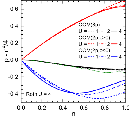
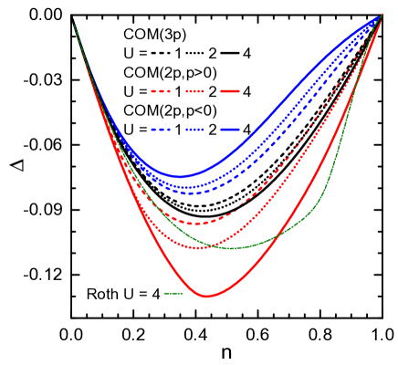
Figure 1: (top) Parameter $p$, diminished of the core term $\frac{1}{4}n^{2}$ of its charge-charge correlation component $\frac{1}{4}\chi_{0}^{\alpha}$, and (bottom) parameter $\Delta$ as functions of the filling $n$ at $U=1$ (dashed lines), $2$ (dotted lines) and $4$ (solid lines) and $T=\nicefrac{{1}}{{6}}$ for COM(3p) (black lines), COM(2p,$p>0$) (red lines) and COM(2p,$p<0$) (blue lines). Roth solution Roth (1969) for $U=4$ (dot-dashed green line) is also reported.

In Fig. 1 (top panel), we report the behavior of the parameter $p$ as a function of the filling $n$ for $U=1$, $2$, $4$ and $T=\nicefrac{{1}}{{6}}$. We subtracted the core, non-fluctuating, term $\frac{1}{4}n^{2}$ of the charge-charge correlation component of $p$, $\frac{1}{4}\chi_{0}^{\alpha}$, in order to be able to better appreciate the effective intensity of the charge, spin and pair fluctuations. The relevance of this parameter, taking into account that we will discuss charge, spin and pair fluctuations in detail in Sec. III.4, is strictly related to its predominant role in the characterization of the $n$-pole solutions available in the literature. Within Hubbard I solution, its value is approximated to just $\frac{1}{4}n^{2}$, which corresponds to a constant value $0$ in Fig. 1 (top panel): no charge, spin or pair fluctuations are taken into account. The two ($p>0$ and $p<0$) two-pole COM(2p) solutions The ; Avella and Mancini (2012b) are named after the sign of $p$ as this latter completely controls the shape of the two Hubbard subbands (see in the following) and, consequently, the whole physical scenario underlying the dynamics of the system. The three-pole solution COM(3p) described in the previous section is characterized by a negative sign of $p-\frac{1}{4}n^{2}$ and by a value of this latter very similar to the one that is possible to find by means of the Roth method Roth (1969), which is actually based on the very same formulas (55), (56) and (57). Although Roth uses the same formulas, the value of $p$ and, in particular, its behavior differs quite much in the most relevant region of filling where the effect of spin fluctuations are expected to be more pronounced. The presence of a third field in the basis ($c_{s}$) changes significantly the values of the correlation functions of the basis and, consequently, those of charge, spin and pair fluctuations. The negative sign of $p-\frac{1}{4}n^{2}$ in COM(3p) is a clear indication of the predominance of spin fluctuations, although with an intensity less pronounced than in COM(2p, $p<0$). Actually, the presence of a minimum (maximum of fluctuation intensity) at a filling significantly lower than $1$ and decreasing with increasing $U$ in COM(2p, $p<0$) is difficult to explain as well as the so large positive value of $p$ in COM(2p, $p>0$). As a matter of fact, in COM(2p) solutions, the parameter $p$ is fixed by an Algebra constraint ($C_{12}=0$) and has lost its physical interpretation inherent to its definition. Its value is just the one necessary to achieve the fulfillment of the Pauli principle at the one-site level (i.e. $n_{\sigma}^{2}\left(i\right)=n_{\sigma}\left(i\right)$) that is so relevant to describe correctly the spin fluctuations and, consequently, catch the virtual processes between nearest-neighbor sites (i.e. the scale of energy of $J=\nicefrac{{4t^{2}}}{{U}}$). In COM(3p), $p-\frac{1}{4}n^{2}$ has just the expected behavior: it smoothly (with respect to Roth, for instance) increases its negative value on reducing doping.

In Fig. 1 (bottom panel), we report the behavior of the parameter $\Delta$ as a function of the filling $n$ for $U=1$, $2$, $4$ and $T=\nicefrac{{1}}{{6}}$. The way to fix this parameter, together with the one used for the parameter $p$, and their resulting values permit to characterize completely all 2-pole solutions present in the literature. Chemical potential $\mu$, the third parameter appearing in any 2-pole treatment, is always fixed by means of the same equation (53) although its value and overall behavior greatly changes according to what is used for $p$ and $\Delta$ (see in the following). Within Hubbard I solution, the value of $\Delta$ is approximated to just $0$: no difference between the kinetic energy contributions of the two Hubbard subbands is taken into account. While the difference between COM solutions as regards this parameter is not so apparent contrarily to what happens for the parameter $p$, it is evident that Roth solution for this parameter reports a behavior quite peculiar. Such a behavior pairs with the one of the parameter $p$ and both cannot be easily explained and are not expected (kinks, changes of concavity, more minima and maxima).

III.2 Local properties and comparison with numerical results

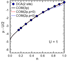
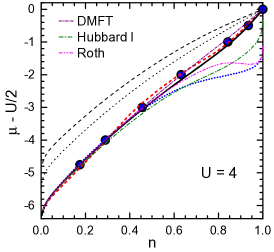
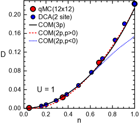
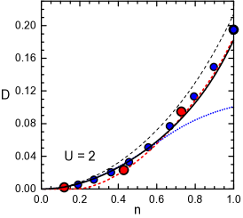
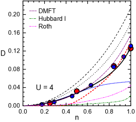
Figure 2: Scaled chemical potential $\mu-\nicefrac{{U}}{{2}}$ (top row) and double occupancy $D$ (bottom row) as functions of the filling $n$ for $U=1$ (left column), $2$ (central column) and $4$ (right column) and $T=\nicefrac{{1}}{{6}}$ for COM(3p) (black lines), COM(2p,$p>0$) (dashed red line) and COM(2p,$p<0$) (dotted blue line). COM results are compared with $12\times 12$-site qMC Moreo et al. (1990) and $2$-site DCA Sangiovanni numerical data (red and blue circles, respectively) as well as with the results of DMFT Capone (dash-dotted purple line), Hubbard I (dot-dashed green line) and Roth (dot-dot-dashed magenta line) methods (only at $U=4$, right column). The thin black dashed and dotted lines in central and right columns are COM(3p) results for $U=1$ and $U=2$, respectively.

In Fig. 2, we report the behavior of the scaled chemical potential $\mu-\nicefrac{{U}}{{2}}$ and of the double occupancy $D$ as functions of the filling $n$ for $U=1$, $2$ and $4$ and $T=\nicefrac{{1}}{{6}}$. It is evident the very good agreement for all values of $U$ reported in the whole range of filling $n$ between COM(3p) and the $12\times 12$-site qMC Moreo et al. (1990) and $2$-site DCA Sangiovanni numerical data. The DCA data for the chemical potential show an apparent change of concavity in proximity of half filling between $U=1,2$ and $U=4$ (Fig. 2 (top row)) that is correctly caught by COM(3p) and COM(2p, $p>0$) and not by COM(2p, $p<0$), Hubbard I and Roth solutions, which always present the same concavity. Roth solution actually reports a rather evident region of thermodynamic instability, $\frac{d\mu}{dn}<0$, close to half filling. As a matter of fact, $U=4$ induces already quite strong electronic correlations, while $U=1,2$ do not: the chemical potential gets ready to open a gap for higher values of $U$ and $n=1$. COM(2p, $p<0$), Hubbard I and Roth solutions not only do not catch the change of concavity in $\mu$, placing themselves always on the strongly correlated side, but they also report values of $\mu$ quite far from the numerical ones: their particle counting - actual effective filling - is definitely far from the exact one. DMFT Capone solution does not catch the change of concavity for $U=4$ either (it will change concavity only for larger values of $U$), but it features values of $\mu$ very close to the numerical ones in the whole range of filling $n$ although not so close as COM(3p) ones in proximity of half-filling, which is the most interesting region. The change of correlation-strength regime between $U=1,2$ and $U=4$ is also quite evident in the behavior of the double occupancy $D$ (Fig. 2 (bottom row)). This latter moves from a parabolic-like behavior somewhat resembling the non-interacting one ($\frac{n^{2}}{4}$) at $U=1,2$ (Fig. 2 (bottom-left/central panels)) to a more elaborated behavior presenting a continuos, but well defined, change of slope on approaching half filling at $U=4$ (Fig. 2 (bottom-right panel)). Again, COM(3p) correctly catches these features, while all other presented solutions do not manage to achieve the same level of agreement over the whole range of filling. Hubbard I and Roth solutions report values of the $D$ extremely far from the numerical ones and always much smaller than these latter, again confirming a tendency to an excess of correlations present in such solutions. DMFT Capone performs extremely well, with respect to numerical data, at low-intermediate values of filling, but at intermediate-high ones features values of $D$ larger than the numerical ones. This is a clear evidence of a lack of correlations for this value of $U$ as shown also by the absence of a change in the concavity of the chemical potential. COM(2p, $p<0$) performs really very well too at low-intermediate values of filling, but on increasing $U$ it shows an excess of correlations close to half filling (it is actually insulating for any finite value of $U$ at half filling - see in the following). COM(2p, $p>0$) is in very good agreement with numerical data for $U=1$ over the whole range of filling, but already for $U=2$, and even more for $U=4$, it is evident a complete suppression of $D$ at low values of the filling as well as a small, but visible, discrepancy in the slope close to half filling for $U=4$. COM(3p) evidently has (see Fig. 2 (bottom-central/right panels)) the capability to correctly interpolate between the two COM(2p) solutions sticking to COM(2p, $p<0$) at low-intermediate values of filling and even improving on COM(2p, $p>0$) at intermediate-high values of filling.

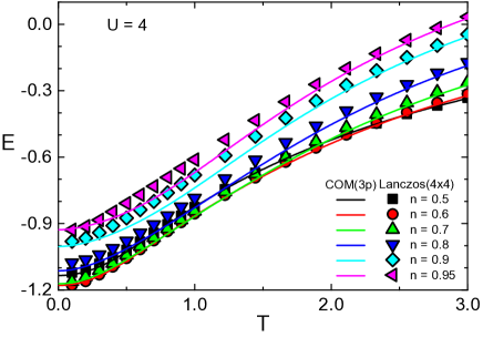
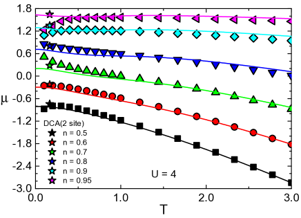
Figure 3: Internal energy per site $E$ (top) and chemical potential $\mu$ (bottom) as functions of the temperature $T$ for various values of the filling $n$ ($0.5\div 0.95$) at $U=4$ for COM(3p) (solid lines), $4\times 4$-site Lanczos Prelovšek (various symbols except stars) and $2$-site DCA Sangiovanni (stars) numerical data.

In Fig. 3, we report the behavior of the internal energy per site $E$ and of the chemical potential $\mu$ as functions of the temperature $T$ for various values of the filling $n$ ($0.5\div 0.95$) at $U=4$. The internal energy per site $E$ has been computed as

$$E=\frac{1}{N}\left\langle H\right\rangle+\mu n=8tC_{cc}^{\alpha}+UD$$ (59)

where $C_{cc}^{\alpha}=\sum_{n,m=1}^{2}C_{nm}^{\alpha}$. Given the very good performance already discussed as regards the double occupancy, this can be seen as a check of the capability of COM(3p) to describe correctly the kinetic energy and, in general, the coherent transport as a function of the temperature. As regards $E$ (Fig. 3 (top panel)), the agreement between COM(3p) and Lanczos Prelovšek is extremely good at high temperatures, where the correlations are weaker and Lanczos results are more reliable, and it is still really very good at low temperatures, where, in particular for low doping, a consistent increase of the correlations is expected. At any rate, the very small discrepancies at low temperatures and small doping cannot be attributed to COM(3p) as the analysis of the chemical potential comparison will clarify. As regards the chemical potential $\mu$ (Fig. 3 (bottom panel)), at high temperatures the agreement between COM(3p) and Lanczos Prelovšek is again excellent, but at low temperatures and for small enough doping the discrepancies between analytical and numerical results are now very much evident and somewhat disturbing. Now, if we add on the same graph (Fig. 3 (bottom panel)) the values obtained for the reported values of the filling by interpolating by means of cubic-splines the related DCA results Sangiovanni ($T=\nicefrac{{1}}{{6}}$ and $U=4$) from Fig. 2 (top row, right column), we clearly see that DCA and Lanczos results agree very well only at high dopings (where also COM(3p) agrees with Lanczos). At low dopings, DCA results evidently differ from Lanczos ones and falls almost exactly on the related COM(3p) lines. It is well known that finite-temperature Lanczos results at low temperatures are not so reliable (they are the result of a high temperature expansion Avella and Mancini (2013)). In this specific case, they seem to indicate the presence of a clear tendency towards a metal-insulator transition for values of $U$ definitely too small: the chemical potential bends towards values significantly lower than $\nicefrac{{U}}{{2}}$ for very small doping. Such a behavior is in contrast with the more reliable - at least in this region of model-parameter space - DCA results and with the rehabilitated COM(3p) ones, which, instead, very well agrees for all values of filling and shows no tendency towards an impending metal-insulator transition.

Figure 4: Double occupancy $D$ as a function of the on-site Coulomb repulsion $U$ for two values of the filling, $n=1$ (top) and $n=\nicefrac{{8}}{{9}}$ (bottom), and three values of the temperature $T$ ($0$, $\nicefrac{{1}}{{16}}$ and $\nicefrac{{1}}{{6}}$) for COM(3p) (black solid and magenta dashed lines), COM(2p,$p>0$) (red dashed line) and COM(2p,$p<0$) (blue dotted line). COM results are compared with $4\times 4$-site qMC White et al. (1989) (black square), $12\times 12$-site qMC Moreo et al. (1990) (green up-triangle), $2$-site DCA Sangiovanni (blue down-triangle), $24\times 24$-site qMC Varney et al. (2009) (red circle in the upper panel) and $3\sqrt{2}\times 3\sqrt{2}$-site Lanczos Becca et al. (2000) (black circle in the lower panel) numerical data.

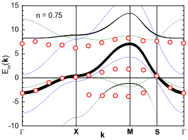
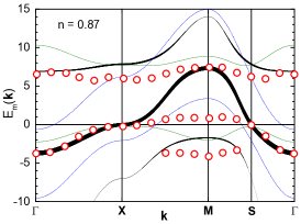
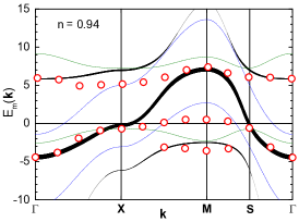
Figure 5: Energy bands $E_{m}\left(\mathbf{k}\right)$ along the principal directions of the first Brillouin zone ($\Gamma=(0,0)$ $\to$ $X=(\pi,0)$ $\to$ $M=(\pi,\pi)$ $\to$ $S=(\nicefrac{{\pi}}{{2}},\nicefrac{{\pi}}{{2}})$ $\to$ $\Gamma=(0,0)$) for $T=0.5$, $U=8$ and three different values of the filling $n=0.75$, $0.87$ and $0.94$ for COM(3p) (variable-thickness black line), COM(2p,$p>0$) (thin dashed blue line) and COM(2p,$p<0$) (thin dotted green line). As regards COM(3p), the thickness of each band is proportional to the value of the corresponding electronic spectral density weight $\sigma_{cc}^{\left(m\right)}\left(\mathbf{k}\right)$ (see in the text). COM results are compared with qMC numerical data Bulut et al. (1994) (red hollow circles).

In Fig. 4, we report the behavior of the double occupancy $D$ as a function of the on-site Coulomb repulsion $U$ for two values of the filling $n$ ($1$ and $\nicefrac{{8}}{{9}}$) and four values of the temperature $T$ ($0$, $\nicefrac{{1}}{{16}}$, $\nicefrac{{1}}{{12}}$ and $\nicefrac{{1}}{{6}}$). First of all, it is worth noting that all reported COM solutions exactly reproduce, by construction, both the $U\rightarrow 0$ and the $U\rightarrow\infty$ limits. At half filling (Fig. 4 (top panel)), COM(3p) results do not show any appreciable difference between the two reported temperatures ($T=\nicefrac{{1}}{{16}}$ and $T=\nicefrac{{1}}{{6}}$) while numerical data show some difference at low values of $U$, where four sets are available at the same time. At low values of $U$, COM(3p) results agree very well with the $12\times 12$-site qMC Moreo et al. (1990), $2$-site DCA Sangiovanni and $24\times 24$-site qMC Varney et al. (2009) data, which are definitely more reliable of the $4\times 4$-site qMC White et al. (1989) data because of both the numerical method used (DCA) and the size of the clusters involved ($12\times 12$ and $24\times 24$). At intermediate-high values of $U$, COM(3p) results agree quite well with both $4\times 4$-site qMC White et al. (1989) and $24\times 24$-site qMC Varney et al. (2009) data, which almost exactly coincide, and agree exactly with both of them for the higher reported values of $U$. At $n=\nicefrac{{8}}{{9}}$ (Fig. 4 (bottom panel)), the agreement between COM(3p) and the $3\sqrt{2}\times 3\sqrt{2}$-site Lanczos Becca et al. (2000) data is quite good and improves more and more on increasing $U$. On the other hand, the overlap of the reported numerical data at half filling and at $n=\nicefrac{{8}}{{9}}$ already in the intermediate range of values of $U$ (we can expect it only at sufficiently high values of $U$) is quite suspect and calls for a revisiting by means of advanced numerical methods applied to larger clusters. Comparing COM(3p) results to COM(2p) ones, we immediately see that COM(3p) overcomes both (i) the very pronounced kink characteristic of COM(2p,$p>0$), signaling the opening of the gap at half-filling and the exit of the chemical potential from the upper Hubbard band at $n=\nicefrac{{8}}{{9}}$, and (ii) the exceedingly small values of $D$ at low and zero doping in COM(2p,$p<0$) already discussed before. The opening of the gap at half-filling and the exit of the chemical potential from the upper Hubbard band at finite doping are strictly equivalent processes with respect to the double occupancy $D$ in COM(2p,$p>0$) as the vast majority of the contribution to $D$ in COM(2p,$p>0$) comes from the upper Hubbard band - see in the following.

III.3 Single-particle properties

In Fig. 5, we report the energy bands $E_{m}\left(\mathbf{k}\right)$ along the principal directions of the first Brillouin zone ($\Gamma=(0,0)$ $\to$ $X=(\pi,0)$ $\to$ $M=(\pi,\pi)$ $\to$ $S=(\nicefrac{{\pi}}{{2}},\nicefrac{{\pi}}{{2}})$ $\to$ $\Gamma=(0,0)$) for $T=0.5$, $U=8$ and three different values of the filling $n=0.75$, $0.87$ and $0.94$. As regards COM(3p), the thickness of each band is proportional to the value of the corresponding electronic spectral density weight $\sigma_{cc}^{\left(m\right)}\left(\mathbf{k}\right)=\sum_{a,b=1}^{2}\sigma_{ab}^{\left(m\right)}\left(\mathbf{k}\right)$. This latter corresponds to the component per band of the momentum distribution function per spin $n\left(\mathbf{k}\right)$ at $T=0$ for those bands and momenta below the chemical potential. Such a decoration shows the effective relevance of each energy bands, momentum per momentum, with respect to actual occupation and possible hole/electron doping. For all three reported values of the filling, COM(3p) results are in very good agreement with qMC numerical data Bulut et al. (1994) as regards the occupied part of the central band (CB). It is worth noticing that this is the most reliable portion of the numerical data as it is close to the chemical potential and tracks the occupied true quasi-particle peak. The lower band (or relic of a band) found by qMC is known as shadow band and has very low intensity. An intensity so low as not to allow a very precise determination of its position, given the very significative broadening of the corresponding peaks. At any rate, this structure is mimed by the LHB in COM(3p), which has a not-negligible occupation right close to $M$ point. On decreasing the doping, this correspondence becomes more and more faithful up to be almost perfect, except for the concavity, at the lower value of the doping ($n=0.94$). The portion of the numerical data closer to the chemical potential at the $M$ point also has not very relevant intensity, but it is important to describe the way the system approaches the metal-insulator transition at half-filling. Unfortunately, this portion of the numerical data is completely missed by COM(3p) solution. This latter also presents a finite occupation of the CB between the two main numerical bands. We can easily recognize that the upper numerical band (whose intensity is significative only close to $M$ point) is very well mimed by the UHB of COM(3p) close to $\Gamma$ point and by the CB close to $M$ point. As well as for the numerical shadow band, on decreasing the doping, the agreement becomes better and better up to be really very good at the lower value of the doping ($n=0.94$) close to both $\Gamma$ and $M$ points. It is worth reminding that qMC data are more and more severely affected by the sign problem on increasing doping: high doping results are less reliable and have larger error bars. As regards the comparison of COM(3p) solution with COM(2p) ones, it is evident the great number and the high level of similarities with the two COM(2p,$p<0$) bands. These latter seem to interpolate somehow between the three COM(3p) bands. It is worth noticing that although COM(2p,$p<0$) bands are really very close to the numerical data in proximity of both the $\Gamma$ point (LHB) and the $M$ point (UHB), COM(3p) bands just lie behind the numerical points in those regions. This clearly shows that the addition of the third field has definitely improved the overall description of the dynamics. COM(2p,$p>0$) bands are simply too different to make any kind of sensible comment.

In Fig. 6 (left and central columns), we report the energy bands $E_{m}\left(\mathbf{k}\right)$ along the principal directions of the first Brillouin zone ($\Gamma=(0,0)$ $\to$ $S=(\nicefrac{{\pi}}{{2}},\nicefrac{{\pi}}{{2}})$ $\to$ $M=(\pi,\pi)$ $\to$ $X=(\pi,0)$ $\to$ $Y=(0,\pi)$ $\to$ $\Gamma=(0,0)$) at $T=\nicefrac{{1}}{{6}}$, $U=4$ and two different values of the filling $n=0.2$ and $n=0.9$. The thickness of each band is proportional to the value of the corresponding electronic spectral density weight $\sigma_{cc}^{\left(m\right)}\left(\mathbf{k}\right)$ in the top row and $\sigma_{22}^{\left(m\right)}\left(\mathbf{k}\right)$ in the bottom row. After (53), (54), (29) and (30), they are the component per band and momentum of the filling $n$ and of double occupancy $D$, respectively, at $T=0$ for those bands and momenta below the chemical potential:

$$n =\sum_{m=1}^{3}n^{\left(m\right)}=\sum\limits_{m=1}^{3}\left[\frac{1}{N}\sum_{\mathbf{k}}f_{\mathrm{F}}\left(E_{m}\left(\mathbf{k}\right)\right)\sigma_{cc}^{\left(m\right)}\left(\mathbf{k}\right)\right]$$ (60)

$$D =\sum_{m=1}^{3}D^{\left(m\right)}=\sum\limits_{m=1}^{3}\left[\frac{1}{N}\sum_{\mathbf{k}}f_{\mathrm{F}}\left(E_{m}\left(\mathbf{k}\right)\right)\sigma_{22}^{\left(m\right)}\left(\mathbf{k}\right)\right]$$ (61)

In Fig. 6 (right column), we report the band component of the filling $n^{\left(m\right)}$ (top-right panel) and of the double occupancy $D^{\left(m\right)}$ (bottom-right panel) as functions of the filling $n$ for the same values of temperature ($T=\nicefrac{{1}}{{6}}$) and on-site Coulomb repulsion ($U=4$).

At $n=0.2$, we expect a significative reduction of the correlations given that the average distance between particles is greater than $2$ lattice spacings. For this filling, it is evident that the bands collecting the vast majority of the electronic occupancy (Fig. 6 (top-left panel)) are almost identical across all reported COM solutions. Looking at $n^{\left(m\right)}$ (Fig. 6 (top-right panel)) for the same value of filling, we immediately realize that actually COM(3p) is characterized by a small, but finite, occupation of its LHB, besides the occupation of its CB, which is the band coinciding with the COM(2p) LHBs. This can be understood in terms of the proximity of COM(3p) LHB to the chemical potential at the $M$ point. There, COM(3p) LHB also features a maximum, that is, a very high density of states (see in the following). Looking instead at $D^{\left(m\right)}$ (Fig. 6 (bottom-right panel)) at $n=0.2$ and cross checking with the $\sigma_{22}^{\left(m\right)}\left(\mathbf{k}\right)$ spectral density (Fig. 6 (bottom-left panel)), we can understand why COM(2p,$p>0$) features a vanishing double occupancy at small fillings (see Fig. 2 (bottom-central/right panels)). Double occupancy is negligible in COM(2p,$p>0$) LHB and all concentrated in the UHB that is all above the chemical potential at small fillings. COM(2p,$p<0$) and COM(3p) LHBs instead contribute significatively to the actual value of the double occupancy at all values of the filling. They contribute almost identically at small and large fillings and very much similarly at intermediate fillings although the actual shape of the bands is quite different away from the $M$ point. As a matter of fact, LHB is the only occupied band in COM(2p,$p<0$) (Fig. 6 (top-right panel)) at all finite values of $U$ (see in the following) and this is the reason why the double occupancy is so small at intermediate and large fillings. Contrarily, at large fillings, COM(3p) can count on the contribution of its CB to the double occupancy, which is greatly enhanced by the proximity of the van Hove singularity to the chemical potential. The composition of these two contributions to the double occupancy (COM(3p) LHB and CB ones) and their quite different behavior with filling (Fig. 6 (bottom-right panel)) can explain the evident change of slope on approaching half filling (see Fig. 2 (bottom row, right column)).

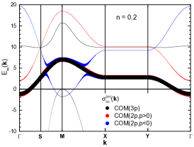
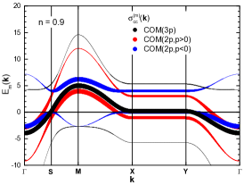
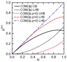
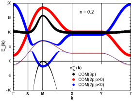
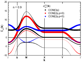
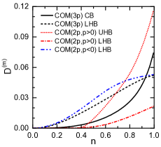
Figure 6: Energy bands $E_{m}\left(\mathbf{k}\right)$ along the principal directions of the first Brillouin zone ($\Gamma=(0,0)$ $\to$ $S=(\nicefrac{{\pi}}{{2}},\nicefrac{{\pi}}{{2}})$ $\to$ $M=(\pi,\pi)$ $\to$ $X=(\pi,0)$ $\to$ $Y=(0,\pi)$ $\to$ $\Gamma=(0,0)$) at $T=\nicefrac{{1}}{{6}}$, $U=4$ and two different values of the filling $n=0.2$ (left column) and $n=0.9$ (central column) for COM(3p) (variable-thickness black line), COM(2p,$p>0$) (variable-thickness red line) and COM(2p,$p<0$) (variable-thickness blue line). The thickness of each band is proportional to the value of the corresponding electronic spectral density weight $\sigma_{cc}^{\left(m\right)}\left(\mathbf{k}\right)$ in the top row and to the value of the corresponding spectral density weight $\sigma_{22}^{\left(m\right)}\left(\mathbf{k}\right)$ in the bottom row. Band components of the filling $n^{\left(m\right)}$ (top-right) and of the double occupancy $D^{\left(m\right)}$ (bottom-right) as functions of the filling $n$ at $T=\nicefrac{{1}}{{6}}$ and $U=4$ for COM(3p) (black lines: CB solid, LHB dashed), COM(2p,$p>0$) (red lines: UHB dotted, LHB dot-dashed) and COM(2p,$p<0$) (blue dot-dot-dashed line).

At $n=0.9$, we expect to be close to the apex of intensity of the electronic correlations. For such a filling, the occupied (with respect to $\sigma_{cc}^{\left(m\right)}\left(\mathbf{k}\right)$: Fig. 6 (top-central panel)) region in energy-momentum space across the three COM solutions is instead quite different, although some similarities can still be found. In particular, as regards the regions close to the chemical potential at the $\Gamma$ point and along the main anti-diagonal (the $X-Y$ line). The behavior of $n^{\left(m\right)}$ (Fig. 6 (top-right panel)) at $n=0.9$ and, in general, at intermediate and large fillings, clearly shows that COM(3p) CB, which was the main actor at low fillings, tends to systematically lose occupation in favor of the LHB. Close to half filling, this latter eventually exceeds the former in occupation and collects more and more of it on increasing $U$ (not shown) while the CB depletes on approaching the metal-insulator transition. As regards COM(2p,$p>0$) instead, UHB plays a minor role all the way up to the metal-insulator transition. It collects a small fraction of the electronic occupation and only above a certain intermediate value of the filling. Moving to the double occupancy $D$, it is worth noticing that the interested regions in energy-momentum space are quite different. COM(3p) receives significant contributions from both the LHB, close to the $M$ point and along the main anti-diagonal (the $X-Y$ line), and the CB, along the main anti-diagonal (the $X-Y$ line). COM(2p,$p<0$) only from the LHB close to the $M$ point. COM(2p,$p>0$) almost only from the UHB close to the $\Gamma$ point. It is now clear why the behavior of the double occupancy among the three COM solutions is very similar (almost identical) at small fillings between COM(3p) and COM(2p,$p<0$) - it comes from particles residing in the very same region in energy-momentum space - and only accidentally similar between COM(3p) and COM(2p,$p>0$) at large fillings.

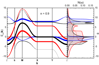
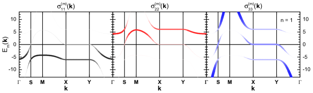
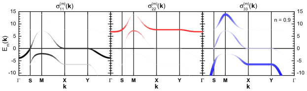
Figure 7: (top) Energy bands $E_{m}\left(\mathbf{k}\right)$ along the principal directions of the first Brillouin zone ($\Gamma=(0,0)$ $\to$ $S=(\nicefrac{{\pi}}{{2}},\nicefrac{{\pi}}{{2}})$ $\to$ $M=(\pi,\pi)$ $\to$ $X=(\pi,0)$ $\to$ $Y=(0,\pi)$ $\to$ $\Gamma=(0,0)$) at $T\cong 0$, $U=8$ and two different values of the filling $n=1$ (left) and $n=0.9$ (right) for COM(3p) (variable-thickness black line), COM(2p,$p>0$) (variable-thickness red line) and COM(2p,$p<0$) (variable-thickness blue line). The thickness of each band is proportional to the value of the corresponding electronic spectral density weight $\sigma_{cc}^{\left(m\right)}\left(\mathbf{k}\right)$. The corresponding densities of states $N\left(\omega\right)$ are reported using thick lines and shaded areas of the same colors: thin dashed, dotted and dot-dashed lines marks the contributions of the various bands. (central-bottom) Energy bands $E_{m}\left(\mathbf{k}\right)$ along the principal directions of the first Brillouin zone ($\Gamma=(0,0)$ $\to$ $S=(\nicefrac{{\pi}}{{2}},\nicefrac{{\pi}}{{2}})$ $\to$ $M=(\pi,\pi)$ $\to$ $X=(\pi,0)$ $\to$ $Y=(0,\pi)$ $\to$ $\Gamma=(0,0)$) at $T\cong 0$, $U=8$ and two different values of the filling $n=1$ (central) and $n=0.9$ (bottom) for COM(3p). The thickness of each band is proportional to the value of the corresponding spectral density weight (left) $\sigma_{11}^{\left(m\right)}\left(\mathbf{k}\right)$, (central) $\sigma_{22}^{\left(m\right)}\left(\mathbf{k}\right)$ and (right) $\sigma_{33}^{\left(m\right)}\left(\mathbf{k}\right)$.

In Fig. 7 (top panels), we report the energy bands $E_{m}\left(\mathbf{k}\right)$ along the principal directions of the first Brillouin zone ($\Gamma=(0,0)$ $\to$ $S=(\nicefrac{{\pi}}{{2}},\nicefrac{{\pi}}{{2}})$ $\to$ $M=(\pi,\pi)$ $\to$ $X=(\pi,0)$ $\to$ $Y=(0,\pi)$ $\to$ $\Gamma=(0,0)$) at $T\cong 0$, $U=8$ and two different values of the filling $n=1$ and $n=0.9$. The thickness of each band is proportional to the value of the corresponding electronic spectral density weight $\sigma_{cc}^{\left(m\right)}\left(\mathbf{k}\right)$. The corresponding density of states, $N\left(\omega\right)=\frac{1}{N}\sum_{\mathbf{k}}\left\{-\frac{1}{\pi}\Im\left[G_{cc}\left(\mathbf{k},\omega\right)\right]\right\}$, is also reported. The latter depends on both the electronic spectral weight, $\sigma_{cc}^{\left(m\right)}\left(\mathbf{k}\right)$, and the effective velocity in the band $m$, $\mathbf{v}_{m}\left(\mathbf{k}\right)=\nabla_{\mathbf{k}}E_{m}\left(\mathbf{k}\right)$,

$$N\left(\omega\right) =\frac{1}{N}\sum_{\mathbf{k}}\sum_{m}\sigma_{cc}^{\left(m\right)}\left(\mathbf{k}\right)\delta\left(\omega-E_{m}\left(\mathbf{k}\right)\right)$$

$$=\sum_{p}\left\|\mathbf{v}_{m}\left(\mathbf{k}_{m}^{\left(p\right)}\left(\omega\right)\right)\right\|^{-1}\sigma_{cc}^{\left(m\right)}\left(\mathbf{k}_{m}^{\left(p\right)}\left(\omega\right)\right)$$ (62)

where $\mathbf{k}_{m}^{\left(p\right)}\left(\omega\right)$ are the zeros of $\omega-E_{m}\left(\mathbf{k}\right)=0$.

At $n=1$ (Fig. 7 (top-left panel)), COM(3p) CB is pinned to the chemical potential along the main anti-diagonal (the $X-Y$ line). The corresponding van Hove singularity in the density of states lies exactly at the Fermi level and the Luttinger theorem is satisfied. Three is the minimal number of poles necessary to satisfy the Luttinger theorem in the Hubbard model. The van Hove peak at the chemical potential gets weaker and weaker on increasing $U$ (not shown), completely disappears only for $U\rightarrow\infty$, and its weight becomes almost negligible with respect to that in the Hubbard subbands for values of U as large as 12, which is the critical value for the metal-insulator transition in COM(2p,$p>0$). This signals an absence of a net transition, but it also manifests a clear tendency towards it.

This is the main drawback of having chosen as third field $c_{s}$ that is not an eigenoperator of the interacting term of the Hamiltonian (1) and, consequently, does not interpret exactly the scale of energy of $U$. Choosing the whole $\pi$ would not have solved this, obviously. The introduction of $c_{s}$ as third field in the operatorial basis improves enormously - up to making it practically exact in many cases - the description of momentum-integrated quantities. This clearly implies that the overall physical content of the chosen third field is exactly what was needed to definitely improve the two-pole solutions through a better description of the nearest-neighbor spin-spin correlations (i.e. of the energy scale of $J=\nicefrac{{4t^{2}}}{{U}}$). On the other hand, the analysis of COM(3p) bands shows that the CB does not reflect correctly the energy scale of $U$ instead, at least as regards its central portion. On increasing $U$, CB stretches out (not shown) keeping its maximum (the $M$ point) at about $\nicefrac{{U}}{{2}}$ and its minimum (the $\Gamma$ point) at about $-\nicefrac{{U}}{{2}}$, that is, within the UHB and the LHB, respectively, while the spectral weight moves rapidly from the central portion, pinned at the chemical potential, towards the extrema. The CB would like to split in two - following its $\xi$ and $\eta$ components - and open up a gap of the order $U$, but it never manages to do so up to $U\rightarrow\infty$ because of its $c$-like component, that is, of the component not resolved in $U$ as in a mean-field treatment of the model.

This is also shown by the spectral weight decoration, according to the three fields of the basis, of COM(3p) bands in Fig. 7 (central panel). It is worth reminding that $\sigma_{33}^{\left(m\right)}\left(\mathbf{k}\right)$ does not directly enter $\sigma_{cc}^{\left(m\right)}\left(\mathbf{k}\right)$, yet it is the best measure of which regions in the energy-momentum space are more affected by $c_{s}$. On one hand, the presence of $c_{s}$ in the basis allows to access those states missing in the two-pole description and resulting in an almost exact description of many relevant quantities. On the other hand, the energy-momentum relation/position of some of these states is simply wrong on the energy scale of $U$. Integrating over momentum this is not so relevant, but becomes evident resolving the bands of the system. As a matter of fact, COM(3p) solution performs so well that is worth analyzing it in detail in order to deeply understand its relevant ingredients so to have an absolutely preferential starting point to improve upon it as regards just this single issue. Along this line, it is very remarkable that COM(3p) CB exactly coincide with COM(2p,$p<0$) LHB and UHB at the $\Gamma$ and the $M$ points, respectively, as well as COM(3p) LHB and UHB are very close (just concavity differs) to COM(2p,$p<0$) LHB and UHB at the $M$ and the $\Gamma$ points, respectively. It is rather evident that, as regards the physics of the lower and upper Hubbard bands, that is, the physics at the scale of energy of $U$, COM(3p) builds upon COM(2p,$p<0$). COM(2p,$p>0$) simply describes a different physics and it is very difficult to compare the two solutions. Looking now at the density of states, it is clear that COM(3p), as well as COM(2p,$p<0$), features peaks in the LHB and in the UHB with the expected strong reduction of the bandwidth from $8t$ to something of the order $J$ according to the reduced mobility of the electrons in a strongly correlated almost-antiferromagnetic background. This is also reflected by the very strong asymmetry, in shape and occupation, with respect to the main anti-diagonal in the LHB and in the UHB.

At $n=0.9$ (Fig. 7 (top-right panel)), it is evident that COM(3p) CB is still almost pinned to the chemical potential along the main anti-diagonal (the $X-Y$ line); the van Hove singularity lies little below the Fermi level. Accordingly, changing the filling in this region of low doping (from $n=0.85$ to $n=1$) has mainly the effect to induce a transfer of spectral weight between the bands and between their components in terms of fields of the basis, as one would expect in a strongly correlated regime, rather than shifting the chemical potential more or less rigidly within the bands, as it could be expected at small fillings and weak interactions. It is also evident, looking at the density of states too, that the LHB has still a minor role with respect to the CB, which collects the vast majority of the occupied states, as also shown by the spectral weight decoration of COM(3p) bands in Fig. 7 (bottom panel). It is worth noting that the spin-spin correlations are already present, but not yet so strong to determine the reduction of the bandwidth in the energy-momentum space region shared by CB and LHB. As well as at $n=1$, although less because of the lack of particle-hole symmetry that is ruling the physics at half filling, COM(3p) bands are quite close to COM(2p,$p<0$) ones.

III.4 Charge, spin and pair correlation functions

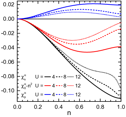
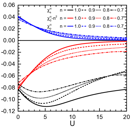
Figure 8: Spin $\chi_{s}^{\alpha}$ (black lines), charge $\chi_{0}^{\alpha}$ (red lines) and pair $\chi_{p}^{\alpha}$ (blue lines) nearest-neighbor correlation functions as functions of filling $n$ (top) and on-site Coulomb repulsion $U$ (bottom) at $T\approxeq 0$ for different values of $U$ ((solid lines) $4$, (dashed lines) $8$ and (dotted lines) $12$) and $n$ ((solid lines) $0.7$, (dashed lines) $0.8$, (dotted lines) $0.9$ and (dot-dashed lines) $1$), respectively. Charge nearest-neighbor correlation function $\chi_{0}^{\alpha}$ has been diminished of its core non-fluctuating value $n^{2}$.

In Fig. 8, we report the spin $\chi_{s}^{\alpha}$, charge $\chi_{0}^{\alpha}$ and pair $\chi_{p}^{\alpha}$ nearest-neighbor correlation functions as functions of filling $n$ and on-site Coulomb repulsion $U$ at $T\approxeq 0$ for different values of $U$ ($4$, $8$ and $12$) and $n$ ($0.7$, $0.8$, $0.9$ and $1$), respectively. Charge nearest-neighbor correlation function $\chi_{0}^{\alpha}$ has been diminished of its core non-fluctuating value $n^{2}$ in order to put all three correlation functions on the same fluctuation footing and make possible a direct comparison of their values.

The first and more relevant consideration that can be drawn looking at both panels at once regards the evident and net predominance of the spin correlations over the charge and pair ones in the relevant range of doping and on-site Coulomb repulsion. This justifies a posteriori the choice of $c_{s}$ as third field in the basis instead of $\pi$ or of any other of its components (charge or pair).

Spin correlations monotonically increase with filling reaching their maximum at half filling as expected. On approaching half filling, an increasing on-site Coulomb repulsion has two main competing effects. On one side, one needs a value of $U$ large enough to establish the perturbative virtual process at the basis of the appearance of the scale of energy of $J=\nicefrac{{4t^{2}}}{{U}}$. On the other side, $J$ is inversely proportional to $U$ and can simply vanish for high enough values of this latter or just become too small to induce strong enough antiferromagnetic correlations in presence of sufficiently high doping. This occurrence has the obvious effect to frustrate the antiferromagnetic order. Too high values of $U$ tend to forbid the virtual process and to favor a ferromagnetic order at half filling instead of an antiferromagnetic one. These facts can explain the quite strange behavior at $U=12$, already somewhat visible at $U=8$. Spin correlations are weaker at $U=12$ than at smaller values of $U$, in particular at large-intermediate doping, then suddenly increase much faster for small enough doping. At half filling, any not exceedingly small value of $J$ favors an antiferromagnetic ordering. In order to reach a full understanding of the reported results, it should be taken into account that we are studying just the homogeneous paramagnetic phase and no real ordering can be expected. Charge and pair correlations feature a maximum around $n=0.5$, where a checkerboard charge order or a double-checkerboard pair order could establish, and tend to vanish at half filling on increasing the on-site Coulomb repulsion that quenches all their fluctuations.

As a function of the on-site Coulomb repulsion $U,$ $\chi_{s}^{\alpha}$ presents a behavior that perfectly agrees with the previous explanation. For small increasing values of $U$, spin correlations also increase following the systematic growth of the number of single-occupied sites. For large increasing values of $U$, spin correlations decrease following the systematic reduction of $J$. In between, $\chi_{s}^{\alpha}$ crosses its maximum at a critical value of $U$ that depends on the value of the filling and on the homogenous-paramagnetic boundary conditions. In fact, we can expect a higher critical value if true antiferromagnetic order would be allowed. It can be inferred that, for small enough doping, the spin correlations will turn positive (ferromagnetic) for sufficiently high values of $U$. It is also evident that half filling is quite special as the spin correlations remain stronger and antiferromagnetic for much higher values of $U$. Charge and pair correlations, instead, systematically decrease on reducing the doping and increasing the on-site Coulomb repulsion showing how their fluctuations completely quench on approaching the metal-insulator transition.

IV Summary and Outlook

We have presented and analyzed in detail a three-pole solution for the two-dimensional Hubbard model within the Composite Operator method framework. The third field, after the two Hubbard ones, has been chosen according to the hierarchy of the equations of motion, but picking up only the operatorial term related to spin correlations/fluctuations in order to both simplify the calculations and highlight the most relevant physics. It is worth noticing that charge and pair operatorial terms have been just projected on the basis chosen and not simply neglected. This choice is justified and promoted, a posteriori, by the very good results obtained in the reported comprehensive comparison with the data obtained by different numerical methods for momentum-integrated quantities (e.g. local properties) as functions of all model parameters (filling, on-site Coulomb repulsion and temperature) as well as for the energy bands of the system. Spin correlations, as expected, are also shown to be the most relevant in intensity and the richest in features so to self-consistently validate the basis choice. The proposed solution has shown to be able to catch many relevant features of the numerical data: the crossover between weak and intermediate-strong correlations on varying both filling and on-site Coulomb repulsion, the way to approach the Mott-Hubbard metal-insulator transition, the presence and energy position of shadow bands, and the exact shape of the occupied portion of the dispersion. A comprehensive comparison with other two-pole solutions has been also reported in order to better understand the ultimate reasons of the very successful comparison with the numerical data and to characterize the proposed solution within the n-pole framework. On one hand, it is evident that the physical content of the chosen third field is driving all improvements and seems exhaustive as regards many relevant properties of the system under analysis so to grant the right for, actually to call for the need of, a comprehensive analysis to this solution. On the other hand, it is also clear that the shape/behavior of the energy-momentum dispersion close to the chemical potential at half filling dictated by the actual choice of the third field suffers from this latter not being an eigenoperator of the interacting term of the Hamiltonian. The field has the right momentum-integrated physical content, but not the exact momentum-resolved one. This can definitely be improved with some efforts in reconsidering the algebra of the operatorial fields involved and we are actually working on this. At any rate, this solution performs already very well as regards many of the relevant properties of the analyzed model.

Appendix A Operatorial Projection

Any field operator $\phi\left(i\right)$ can be projected on a set of fields operators $\left\{\psi_{m}\left(i\right)\right\}$ featuring $I_{\psi_{m}\psi_{p}}\left(\mathbf{i},\mathbf{j}\right)=\delta_{mp}\delta_{\mathbf{ij}}I_{\psi_{m}\psi_{m}}$ (e.g. $\left\{\xi\left(i\right),\eta\left(i\right)\right\}$) through the following relation

$$\phi\left(i\right)\cong\sum_{m}\sum_{\mathbf{j}}\frac{I_{\phi\psi_{m}}\left(\mathbf{i},\mathbf{j}\right)}{I_{\psi_{m}\psi_{m}}}\psi_{m}\left(\mathbf{j},t\right)$$ (63)

We can rewrite $\chi_{s}^{\alpha}$ and $f_{s}$ as follows (we extracted first the component of $f_{s}$ involving only two sites: $-\frac{1}{2}C_{c\xi}^{\alpha}$)

$$\chi_{s}^{\alpha} =-\frac{1}{3}\operatorname{Tr}\left\langle\phi_{s}\left(i\right)\otimes c^{\dagger}\left(i\right)\right\rangle$$ (64)

$$f_{s} =-\frac{1}{2}C_{c\xi}^{\alpha}-\frac{1}{6}\operatorname{Tr}\left\langle\phi_{s}\left(i\right)\otimes c^{\dagger\alpha\left(\beta\right)}\left(i\right)\right\rangle$$

$$-\frac{1}{12}\operatorname{Tr}\left\langle\phi_{s}\left(i\right)\otimes c^{\dagger\alpha\left(\eta\right)}\left(i\right)\right\rangle$$ (65)

where $\phi_{s}\left(i\right)=n_{k}^{\alpha}\left(i\right)\sigma_{k}\cdot c\left(i\right)$. $\left(\varrho^{\alpha}\left(i\right)\otimes\right)\varphi^{\alpha\left(\beta\right)}\left(i\right)$ and $\left(\varrho^{\alpha}\left(i\right)\otimes\right)\varphi^{\alpha\left(\eta\right)}\left(i\right)$ stand for an operator $\varphi$ sited on a site that is nearest-neigbor ($\alpha$) of site $\mathbf{i}$ and second-nearest-neighbor ($\beta$ and $\eta$, respectively) of the actual site where the operator $\varrho$ is sited (e.g. $\varrho^{\alpha}\left(i\right)\otimes\varphi^{\alpha\left(\beta\right)}\left(i\right):$ $\varrho\left(i\pm\hat{x}\right)\otimes\varphi\left(i\pm\hat{y}\right)$, $\varrho^{\alpha}\left(i\right)\otimes\varphi^{\alpha\left(\eta\right)}\left(i\right):$ $\varrho\left(i\pm\hat{x}\right)\otimes\varphi\left(i\mp\hat{x}\right)$).

Choosing $\left\{\xi\left(i\right),\eta\left(i\right)\right\}$ as set of fields operators $\left\{\psi_{m}\left(i\right)\right\}$, we have the following relevant relations

$$I_{\phi_{s}\xi}\left(\mathbf{i},\mathbf{j}\right) =\frac{3}{2}\delta_{\mathbf{ij}}\chi_{s}^{\alpha}+3\alpha_{\mathbf{ij}}C_{c\xi}^{\alpha}$$ (66)

$$I_{\phi_{s}\eta}\left(\mathbf{i},\mathbf{j}\right) =-\frac{3}{2}\delta_{\mathbf{ij}}\chi_{s}^{\alpha}+3\alpha_{\mathbf{ij}}C_{c\eta}^{\alpha}$$ (67)

Accordingly, we have the following projection for the field $\phi_{s}\left(i\right)$

$$\phi_{s}\left(i\right)\cong\frac{3}{2}\frac{\chi_{s}^{\alpha}}{I_{11}}\xi\left(i\right)-\frac{3}{2}\frac{\chi_{s}^{\alpha}}{I_{22}}\eta\left(i\right)+3\frac{C_{c\xi}^{\alpha}}{I_{11}}\xi^{\alpha}\left(i\right)+3\frac{C_{c\eta}^{\alpha}}{I_{22}}\eta^{\alpha}\left(i\right)$$ (68)

that leads to the following closed relation for $\chi_{s}^{\alpha}$ (leading to (56))

$$\chi_{s}^{\alpha}\cong-\frac{\chi_{s}^{\alpha}}{I_{11}}C_{\xi\xi}+\frac{\chi_{s}^{\alpha}}{I_{22}}C_{\eta\eta}-2\frac{C_{c\xi}^{\alpha}}{I_{11}}C_{c\xi}^{\alpha}-2\frac{C_{c\eta}^{\alpha}}{I_{22}}C_{c\eta}^{\alpha}$$ (69)

and to the expression of $f_{s}$ in the main text (58). To get this latter, we used the geometrical relation $C_{\phi\psi}^{\alpha^{2}}=\frac{1}{4}C_{\phi\psi}+\frac{1}{2}C_{\phi\psi}^{\beta}+\frac{1}{4}C_{\phi\psi}^{\eta}$.

In the very same way, we can rewrite $\chi_{0}^{\alpha}$ as follows

$$\chi_{0}^{\alpha}=2n-\operatorname{Tr}\left\langle\phi_{0}\left(i\right)\otimes c^{\dagger}\left(i\right)\right\rangle$$ (70)

where $\phi_{0}\left(i\right)=n^{\alpha}\left(i\right)c\left(i\right)$. Using the very same set of fields operators, we have the following relevant relations

$$I_{\phi_{0}\xi}\left(\mathbf{i},\mathbf{j}\right) =\delta_{\mathbf{ij}}\left(n-\frac{1}{2}\chi_{0}^{\alpha}\right)+\alpha_{\mathbf{ij}}C_{c\xi}^{\alpha}$$ (71)

$$I_{\phi_{0}\eta}\left(\mathbf{i},\mathbf{j}\right) =\frac{1}{2}\delta_{\mathbf{ij}}\chi_{0}^{\alpha}+\alpha_{\mathbf{ij}}C_{c\eta}^{\alpha}$$ (72)

Accordingly, we have the following projection for the field $\phi_{0}\left(i\right)$

$$\phi_{0}\left(i\right)\cong\frac{n-\frac{1}{2}\chi_{0}^{\alpha}}{I_{11}}\xi\left(i\right)+\frac{1}{2}\frac{\chi_{0}^{\alpha}}{I_{22}}\eta\left(i\right)+\frac{C_{c\xi}^{\alpha}}{I_{11}}\xi^{\alpha}\left(i\right)+\frac{C_{c\eta}^{\alpha}}{I_{22}}\eta^{\alpha}\left(i\right)$$ (73)

that leads to the following closed relation for $\chi_{0}^{\alpha}$ (leading to (55))

$$\chi_{0}^{\alpha}\cong 2n-\frac{2n-\chi_{0}^{\alpha}}{I_{11}}C_{\xi\xi}-\frac{\chi_{0}^{\alpha}}{I_{22}}C_{\eta\eta}-2\frac{C_{c\xi}^{\alpha}}{I_{11}}C_{c\xi}^{\alpha}-2\frac{C_{c\eta}^{\alpha}}{I_{22}}C_{c\eta}^{\alpha}$$ (74)

Once more, we can rewrite $\chi_{p}^{\alpha}$ as follows

$$\chi_{p}^{\alpha}=\left\langle\phi_{p}\left(i\right)c_{\uparrow}^{\dagger}\left(i\right)\right\rangle$$ (75)

where $\phi_{p}\left(i\right)=\left[c_{\uparrow}\left(i\right)c_{\downarrow}\left(i\right)\right]^{\alpha}c_{\downarrow}^{\dagger}\left(i\right)$. Using the very same set of fields operators, we have the following relevant relations

$$I_{\phi_{p}\xi}\left(\mathbf{i},\mathbf{j}\right) =\delta_{\mathbf{ij}}\chi_{p}^{\alpha}+\alpha_{\mathbf{ij}}C_{c\eta}^{\alpha}$$ (76)

$$I_{\phi_{p}\eta}\left(\mathbf{i},\mathbf{j}\right) =-\delta_{\mathbf{ij}}\chi_{p}^{\alpha}+\alpha_{\mathbf{ij}}C_{c\xi}^{\alpha}$$ (77)

Accordingly, we have the following projection for the field $\phi_{p0}\left(i\right)$

$$\phi_{p}\left(i\right)\cong\frac{\chi_{p}^{\alpha}}{I_{11}}\xi\left(i\right)-\frac{\chi_{p}^{\alpha}}{I_{22}}\eta\left(i\right)+\frac{C_{c\eta}^{\alpha}}{I_{11}}\xi^{\alpha}\left(i\right)+\frac{C_{c\xi}^{\alpha}}{I_{22}}\eta^{\alpha}\left(i\right)$$ (78)

that leads to the following closed relation for $\chi_{p}^{\alpha}$ (leading to (57))

$$\chi_{p}^{\alpha}\cong\frac{\chi_{p}^{\alpha}}{I_{11}}C_{\xi\xi}-\frac{\chi_{p}^{\alpha}}{I_{22}}C_{\eta\eta}+\frac{C_{c\eta}^{\alpha}}{I_{11}}C_{c\xi}^{\alpha}+\frac{C_{c\xi}^{\alpha}}{I_{22}}C_{c\eta}^{\alpha}$$ (79)

References

- Hubbard (1963) J. Hubbard, Proc. Roy. Soc. A 276, 238 (1963).
- Imada et al. (1998) M. Imada, A. Fujimori, and Y. Tokura, Rev. Mod. Phys. 70, 1039 (1998).
- Bednorz and Müller (1986) J. G. Bednorz and K. A. Müller, Z. Phys. B 64, 189 (1986).
- Anderson (1987) P. W. Anderson, Science 235, 1196 (1987).
- Alloul et al. (1989) H. Alloul, T. Ohno, and P. Mendels, Phys. Rev. Lett. 63, 1700 (1989).
- Timusk and Statt (1999) T. Timusk and B. Statt, Rep. Prog. Phys. 62, 61 (1999).
- Basov et al. (1999) D. N. Basov, S. I. Woods, A. S. Katz, E. J. Singley, R. C. Dynes, M. Xu, D. G. Hinks, C. C. Homes, and M. Strongin, Science 283, 49 (1999).
- Orenstein and Millis (2000) J. Orenstein and A. J. Millis, Science 288, 468 (2000).
- Damascelli et al. (2003) A. Damascelli, Z. Hussain, and Z.-X. Shen, Rev. Mod. Phys. 75, 473 (2003).
- Shen et al. (2005) K. M. Shen et al., Science 307, 901 (2005).
- Eschrig (2006) M. Eschrig, Adv. Phys. 55, 47 (2006).
- Kanigel et al. (2006) A. Kanigel et al., Nature Phys. 2, 447 (2006).
- Lee et al. (2006) P. A. Lee, N. Nagaosa, and X.-G. Wen, Rev. Mod. Phys. 78, 17 (2006).
- Valla et al. (2006) T. Valla, A. V. Fedorov, J. Lee, J. C. Davis, and G. D. Gu, Science 314, 1914 (2006).
- Doiron-Leyraud et al. (2007) N. Doiron-Leyraud, C. Proust, D. LeBoeuf, J. Levallois, J.-B. Bonnemaison, R. X. Liang, D. A. Bonn, W. N. Hardy, and L. Taillefer, Nature 447, 565 (2007).
- LeBoeuf et al. (2007) D. LeBoeuf et al., Nature 450, 533 (2007).
- Bangura et al. (2008) A. F. Bangura et al., Phys. Rev. Lett. 100, 047004 (2008).
- Hossain et al. (2008) M. A. Hossain et al., Nature Phys. 4, 527 (2008).
- Yelland et al. (2008) E. A. Yelland, J. Singleton, C. H. Mielke, N. Harrison, F. F. Balakirev, B. Dabrowski, and J. R. Cooper, Phys. Rev. Lett. 100, 047003 (2008).
- Sebastian et al. (2008) S. E. Sebastian, N. Harrison, E. Palm, T. P. Murphy, C. H. Mielke, R. X. Liang, D. A. Bonn, W. N. Hardy, and G. G. Lonzarich, Nature 454, 200 (2008).
- Audouard et al. (2009) A. Audouard, C. Jaudet, D. Vignolles, R. X. Liang, D. A. Bonn, W. N. Hardy, L. Taillefer, and C. Proust, Phys. Rev. Lett. 103, 157003 (2009).
- Meng et al. (2009) J. Q. Meng et al., Nature 462, 335 (2009).
- Anzai et al. (2010) H. Anzai et al., Phys. Rev. Lett. 105, 227002 (2010).
- Singleton et al. (2010) J. Singleton et al., Phys. Rev. Lett. 104, 086403 (2010).
- Sebastian et al. (2010a) S. E. Sebastian, N. Harrison, C. H. Altarawneh, R. X. Liang, D. A. Bonn, W. N. Hardy, and G. G. Lonzarich, Phys. Rev. B 81, 140505 (2010a).
- Sebastian et al. (2010b) S. E. Sebastian, N. Harrison, M. M. Altarawneh, P. A. Goddard, C. H. Mielke, R. X. Liang, D. A. Bonn, W. N. Hardy, and G. G. Lonzarich, Phys. Rev. B 81, 140505 (2010b).
- Sebastian et al. (2010c) S. E. Sebastian, N. Harrison, M. M. Altarawneh, C. H. Mielke, R. X. Liang, D. A. Bonn, W. N. Hardy, and G. G. Lonzarich, Proc. Nat. Acad. Sci. USA 107, 6175 (2010c).
- Tranquada et al. (2010) J. M. Tranquada, D. N. Basov, A. D. LaForge, and A. A. Schafgans, Phys. Rev. B 81, 060506 (2010).
- Vishik et al. (2010) I. M. Vishik et al., Phys. Rev. Lett. 104, 207002 (2010).
- King et al. (2011) P. D. C. King et al., Phys. Rev. Lett. 106, 127005 (2011).
- Laliberte et al. (2011) F. Laliberte et al., Nature Commun. 2, 432 (2011).
- Ramshaw et al. (2011) B. J. Ramshaw, B. Vignolle, J. Day, R. X. Liang, W. N. Hardy, C. Proust, and D. A. Bonn, Nature Phys. 7, 234 (2011).
- Riggs et al. (2011) S. C. Riggs, O. Vafek, J. B. Kemper, J. B. Betts, A. Migliori, F. F. Balakirev, W. N. Hardy, R. X. Liang, D. A. Bonn, and G. S. Boebinger, Nature Phys. 7, 332 (2011).
- Sebastian et al. (2011a) S. E. Sebastian, N. Harrison, M. M. Altarawneh, F. F. Balakirev, C. H. Mielke, R. Liang, D. A. Bonn, W. N. Hardy, and G. G. Lonzarich (2011a), arXiv:1103.4178.
- Sebastian et al. (2011b) S. E. Sebastian, N. Harrison, M. M. Altarawneh, R. Liang, D. A. Bonn, W. N. Hardy, and G. G. Lonzarich, Nature Commun. 2, 471 (2011b).
- Sebastian et al. (2011c) S. E. Sebastian, N. Harrison, and G. G. Lonzarich, Phil. Trans. R. Soc. London A 369, 1687 (2011c).
- Vignolle et al. (2011) B. Vignolle et al., C. R. Physique 12, 446 (2011).
- Sebastian et al. (2012a) S. E. Sebastian, N. Harrison, R. Liang, D. A. Bonn, W. N. Hardy, C. Mielke, and G. G. Lonzarich, Phys. Rev. Lett. 108, 196403 (2012a).
- Sebastian et al. (2012b) S. E. Sebastian, N. Harrison, and G. G. Lonzarich, Rep. Prog. Phys. 75, 102501 (2012b).
- Tremblay et al. (2006) A.-M. S. Tremblay, B. Kyung, and D. Sénéchal, Fizika Nizkikh Temperatur 32, 561 (2006), (Low Temp. Phys. 32, 424 (2006)).
- Avella and Mancini (2013) A. Avella and F. Mancini, eds., Strongly Correlated Systems: Numerical Methods, vol. 176 of Springer Series in Solid-State Sciences (Springer Berlin Heidelberg, 2013).
- Avella and Mancini (2012a) A. Avella and F. Mancini, eds., Strongly Correlated Systems: Theoretical Methods, vol. 171 of Springer Series in Solid-State Sciences (Springer Berlin Heidelberg, 2012a).
- Mori (1965) H. Mori, Prog. Theor. Phys. 33, 423 (1965).
- Hubbard (1964a) J. Hubbard, Proc. Roy. Soc. A 277, 237 (1964a).
- Hubbard (1964b) J. Hubbard, Proc. Roy. Soc. A 281, 401 (1964b).
- Rowe (1968) D. J. Rowe, Rev. Mod. Phys. 40, 153 (1968).
- Roth (1969) L. M. Roth, Phys. Rev. 184, 451 (1969).
- Tserkovnikov (1981a) Y. A. Tserkovnikov, Teor. Mat. Fiz. 49, 219 (1981a).
- Tserkovnikov (1981b) Y. A. Tserkovnikov, Teor. Mat. Fiz. 50, 261 (1981b).
- Gutzwiller (1963) M. C. Gutzwiller, Phys. Rev. Lett. 10, 159 (1963).
- Gutzwiller (1964) M. C. Gutzwiller, Phys. Rev. 134, A923 (1964).
- Gutzwiller (1965) M. C. Gutzwiller, Phys. Rev. 137, A1726 (1965).
- Brinkman and Rice (1970) W. F. Brinkman and T. M. Rice, Phys. Rev. B 2, 4302 (1970).
- Yokoyama and Shiba (1987) H. Yokoyama and H. Shiba, J. Phys. Soc. Jpn. 56, 1490 (1987).
- Gulácsi et al. (1993) Z. Gulácsi, R. Strack, and D. Vollhardt, Phys. Rev. B 47, 8594 (1993).
- Bünemann and Weber (1997) J. Bünemann and W. Weber, Phys. Rev. B 55, 4011 (1997).
- Dzierzawa et al. (1997) M. Dzierzawa, D. Baeriswyl, and S. Martelo, Helv. Phys. Acta 70, 124 (1997).
- Bünemann et al. (1998) J. Bünemann, W. Weber, and F. Gebhard, Phys. Rev. B 57, 6896 (1998).
- Seibold et al. (2003) G. Seibold, F. Becca, and J. Lorenzana, Phys. Rev. B 67, 085108 (2003).
- Attaccalite and Fabrizio (2003) C. Attaccalite and M. Fabrizio, Phys. Rev. B 68, 155117 (2003).
- Ferrero et al. (2005) M. Ferrero, F. Becca, M. Fabrizio, and M. Capone, Phys. Rev. B 72, 205126 (2005).
- Capello et al. (2005) M. Capello, F. Becca, M. Fabrizio, S. Sorella, and E. Tosatti, Phys. Rev. Lett. 94, 026406 (2005).
- Fabrizio (2007) M. Fabrizio, Phys. Rev. B 76, 165110 (2007).
- Lanatà et al. (2008) N. Lanatà, P. Barone, and M. Fabrizio, Phys. Rev. B 78, 155127 (2008).
- Ho et al. (2008) K. M. Ho, J. Schmalian, and C. Z. Wang, Phys. Rev. B 77, 073101 (2008).
- Deng et al. (2009) X. Deng, L. Wang, X. Dai, and Z. Fang, Phys. Rev. B 79, 075114 (2009).
- Schiró and Fabrizio (2010) M. Schiró and M. Fabrizio, Phys. Rev. Lett. 105, 076401 (2010).
- Tocchio et al. (2011) L. F. Tocchio, F. Becca, and C. Gros, Phys. Rev. B 83, 195138 (2011).
- Lanatà et al. (2012) N. Lanatà, H. U. R. Strand, X. Dai, and B. Hellsing, Phys. Rev. B 85, 035133 (2012).
- Barnes (1976) S. E. Barnes, J. Phys. F 6, 1375 (1976).
- Coleman (1984) P. Coleman, Phys. Rev. B 29, 3035 (1984).
- Kotliar and Ruckenstein (1986) G. Kotliar and A. E. Ruckenstein, Phys. Rev. Lett. 57, 1362 (1986).
- Kalashnikov and Fradkin (1969) O. K. Kalashnikov and E. S. Fradkin, Sov. Phys. JETP 28, 317 (1969).
- Nolting (1972) W. Nolting, Z. Phys. 255, 25 (1972).
- Chubukov and Norman (2004) A. V. Chubukov and M. R. Norman, Phys. Rev. B 70, 174505 (2004), and references therein.
- Prelovšek and Ramšak (2005) P. Prelovšek and A. Ramšak, Phys. Rev. B 72, 012510 (2005).
- Plakida and Oudovenko (2007) N. M. Plakida and V. S. Oudovenko, JETP 104, 230 (2007).
- Metzner and Vollhardt (1989) W. Metzner and D. Vollhardt, Phys. Rev. Lett. 62, 324 (1989).
- Georges and Kotliar (1992) A. Georges and G. Kotliar, Phys. Rev. B 45, 6479 (1992).
- Georges et al. (1996) A. Georges, G. Kotliar, W. Krauth, and M. J. Rozenberg, Rev. Mod. Phys. 68, 13 (1996).
- Sadovskii et al. (2005) M. V. Sadovskii, I. A. Nekrasov, E. Z. Kuchinskii, T. Pruschke, and V. I. Anisimov, Phys. Rev. B 72, 155105 (2005).
- Kuchinskii et al. (2005) E. Z. Kuchinskii, I. A. Nekrasov, and M. V. Sadovskii, JETP Letters 82, 198 (2005).
- Kuchinskii et al. (2006) E. Z. Kuchinskii, I. A. Nekrasov, and M. V. Sadovskii, Fizika Nizkikh Temperatur 32, 528 (2006).
- Maier et al. (2005) T. Maier, M. Jarrell, T. Pruschke, and M. H. Hettler, Rev. Mod. Phys. 77, 1027 (2005).
- Kotliar et al. (2001) G. Kotliar, S. Y. Savrasov, G. Palsson, and G. Biroli, Phys. Rev. Lett. 87, 186401 (2001).
- Hettler et al. (1998) M. H. Hettler, A. N. Tahvildar-Zadeh, M. Jarrell, T. Pruschke, and H. R. Krishnamurthy, Phys. Rev. B 58, R7475 (1998).
- Sénéchal et al. (2000) D. Sénéchal, D. Perez, and M. Pioro-Ladriére, Phys. Rev. Lett. 84, 522 (2000).
- (88) F. Mancini and A. Avella, Adv. Phys. 53, 537 (2004); Eur. Phys. J. B 36, 37 (2003).
- Avella and Mancini (2012b) A. Avella and F. Mancini, in Strongly Correlated Systems: Theoretical Methods, edited by A. Avella and F. Mancini (Springer Berlin Heidelberg, 2012b), vol. 171 of Springer Series in Solid-State Sciences, p. 103, URL http://dx.doi.org/10.1007/978-3-642-21831-6_4.
- (90) A. Avella, F. Mancini et al., Int. J. Mod. Phys. B 12, 81 (1998); Phys. Rev. B 63, 245117 (2001); Eur. Phys. J. B 29, 399 (2002); Phys. Rev. B 67, 115123 (2003); Eur. Phys. J. B 36, 445 (2003); Physica. C 470, S930 (2010); J. Phys. Chem. Solids 72, 362 (2011).
- Odashima et al. (2005) S. Odashima, A. Avella, and F. Mancini, Phys. Rev. B 72, 205121 (2005).
- (92) A. Avella, F. Mancini, F. P. Mancini, and E. Plekhanov, J. Phys. Chem. Solids 72, 384 (2011); J. Phys.: Conf. Series 273, 012091 (2011); 391, 012121 (2012); Eur. Phys. J. B 86, 265 (2013).
- (93) A. Avella, F. Mancini et al., Phys. Lett. A 240, 235 (1998); Eur. Phys. J. B 20, 303 (2001).
- (94) A. Avella and F. Mancini, Eur. Phys. J. B 41, 149 (2004).
- Villani et al. (2000) D. Villani, E. Lange, A. Avella, and G. Kotliar, Phys. Rev. Lett. 85, 804 (2000).
- (96) A. Avella, F. Mancini, and R. Hayn, Eur. Phys. J. B 37, 465 (2004).
- Plekhanov et al. (2011) E. Plekhanov, A. Avella, F. Mancini, and F. P. Mancini, J. Phys.: Conf. Ser. 273, 012147 (2011).
- (98) A. Avella and F. Mancini, Eur. Phys. J. B 50, 527 (2006).
- Avella et al. (2008) A. Avella, F. Mancini, and E. Plekhanov, Eur. Phys. J. B 66, 295 (2008).
- (100) E. Plekhanov, A. Avella, and F. Mancini, Phys. Rev. B 74, 115120 (2006); Eur. Phys. J. B 77, 381 (2010).
- (101) A. Avella, F. Mancini et. al, Solid State Commun. 108, 723 (1998); Eur. Phys. J. B 32, 27 (2003).
- Avella and Mancini (2007a) A. Avella and F. Mancini, Phys. Rev. B 75, 134518 (2007a).
- Avella and Mancini (2007b) A. Avella and F. Mancini, J. Phys.: Condens. Matter 19, 255209 (2007b).
- Avella and Mancini (2008) A. Avella and F. Mancini, Acta Phys. Pol., A 113, 395 (2008).
- Avella and Mancini (2009) A. Avella and F. Mancini, J. Phys.: Condens. Matter 21, 254209 (2009).
- (106) naturally appears in the equation of motion of the electronic field operator : .
- (107) An eigenoperator of a Hamiltonian , or of one or more terms of this latter, is an operator whose current with respect to , or to one or more terms of this latter, is proportional to the operator itself: . The proportionality constant is named eigenenergy of the eigenoperator with respect to , or to one or more terms of this latter.
- (108) This vector is of the type where the index individuates an operator in the operatorial basis and the index is the spin indices related to the spinorial notation. The summation over these two indexes is usually understood. See also Ref. mat, .
- (109) This matrix is of the type where the indexes and individuate an operator in the operatorial basis and the indexes and are the spin indices related to the spinorial notation. The summation over these four indexes is usually understood. For instance: , .
- (110) The product of two symmetric matrices has real eigenvalues if one of the two is semi-positive, that is, it has positive or null eigenvalues.
- Moreo et al. (1990) A. Moreo, D. J. Scalapino, R. L. Sugar, S. R. White, and N. E. Bickers, Phys. Rev. B 41, 2313 (1990).
- (112) G. Sangiovanni, private communication.
- (113) M. Capone, private communication.
- (114) P. Prelovšek, private communication.
- White et al. (1989) S. R. White, D. J. Scalapino, R. L. Sugar, E. Y. Loh, J. E. Gubernatis, and R. T. Scalettar, Phys. Rev. B 40, 506 (1989).
- Varney et al. (2009) C. N. Varney, C.-R. Lee, Z. J. Bai, S. Chiesa, M. Jarrell, and R. T. Scalettar, Phys. Rev. B 80, 075116 (2009).
- Becca et al. (2000) F. Becca, A. Parola, and S. Sorella, Phys. Rev. B 61, 16287 (2000).
- Bulut et al. (1994) N. Bulut, D. J. Scalapino, and S. R. White, Phys. Rev. B 50, 7215 (1994).