Cross-calibration of Time-of-flight and
Colour Cameras

Abstract

Time-of-flight cameras provide depth information, which is complementary to the photometric appearance of the scene in ordinary images. It is desirable to merge the depth and colour information, in order to obtain a coherent scene representation. However, the individual cameras will have different viewpoints, resolutions and fields of view, which means that they must be mutually calibrated. This paper presents a geometric framework for the resulting multi-view and multi-modal calibration problem. It is shown that three-dimensional projective transformations can be used to align depth and parallax-based representations of the scene, with or without Euclidean reconstruction. A new evaluation procedure is also developed; this allows the reprojection error to be decomposed into calibration and sensor-dependent components. The complete approach is demonstrated on a network of three time-of-flight and six colour cameras. The applications of such a system, to a range of automatic scene-interpretation problems, are discussed.

1 Introduction

The segmentation of multi-view video data, with respect to physically distinct objects of interest, is an essential task in automatic scene-interpretation. Visual segmentation can be based on colour, texture, parallax and motion information (e.g. hoiem-2007 ; tron-2007 ). The task remains very difficult, however, owing to the combined effects of non-rigid surfaces, variable lighting, and occlusion. It has become clear that depth cameras can make an important contribution to scene understanding, by enabling direct depth segmentation, based on the measured scene-structure (see CVIU special issue savarese-2009 ). This approach is also highly effective for dynamic tasks, such as body tracking and action recognition liu-2014 . Furthermore, if depth and colour information can be merged into a single representation, then a complete 3-d representation is possible, in principle. This is clearly desirable, because colour and texture data are essential to many other aspects of scene-understanding, such as identification and tracking alahi-2010 .

There are two major obstacles to the construction of a complete scene representation, from a multi-modal camera network. Firstly, typical depth sensors are unable to capture rgb data mesa-2010 . This means that the depth and colour cameras will have different viewpoints, and so the raw data are inconsistent. Secondly, typical tof and rgb cameras have limited fields of view, and so the depth and colour data are incomplete. This paper addresses both of these problems, by showing how to estimate the geometric relationships in a multi-view, multi-modal camera network. This task will be called cross-calibration.

In order to constrain the problem, two practical constraints are imposed from the outset. Firstly, the system will be based on time-of-flight (tof) cameras, in conjunction with ordinary rgb cameras. The tof cameras are compact, can be properly synchronized, and are industrially specified, e.g., mesa-2010 . Secondly, a modular network of tof+rgb units is required. This is so that individual units can be added or removed, in order to optimize the scene-coverage.

1.1 Overview

Time-of-flight cameras can, in principle, be geometrically calibrated by standard methods hansard-2014 . This means that each pixel records an estimate of the scene-distance (range) along the corresponding ray. The 3-d structure of a scene can also be reconstructed from two or more ordinary images, via the parallax (e.g. binocular disparity) between corresponding image points. There are many advantages to be gained by combining the range and parallax data. Most obviously, each point in a parallax-based reconstruction can be mapped back into the original images, from which colour and texture can be obtained. Parallax-based reconstructions are, however, difficult to obtain, owing to the difficulty of putting the image points into correspondence. Indeed, it may be impossible to find any correspondences in untextured regions. Furthermore, if a Euclidean reconstruction is required, then the cameras must be calibrated. The accuracy of the resulting reconstruction will also tend to decrease with the distance of the scene from the cameras verri-1986 .

The range data, on the other hand, are often corrupted by noise and surface-scattering. The spatial resolution of current tof sensors is relatively low, the depth-range is limited, and the luminance signal may be unusable for rendering and for classical image processing. It should also be recalled that tof cameras, of the type used here, cannot be used in outdoor lighting conditions. These considerations lead to the idea of a mixed colour and time-of-flight system, as described in lindner-2010 . Such a system could, in principle, be used to make high-resolution Euclidean reconstructions, including photometric information kolb-2010 ; gandhi-2012 .

In order to make full use of a mixed range/parallax system, it is necessary to find the exact geometric relationship between the different devices. In particular, the reprojection of the tof data, into the colour images, must be obtained. This paper is concerned with the estimation of these geometric relationships. Specifically, the aim is to align the range and parallax reconstructions, by a suitable 3-d transformation.

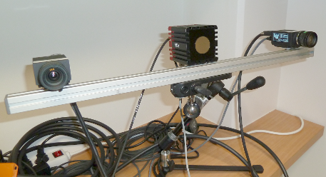
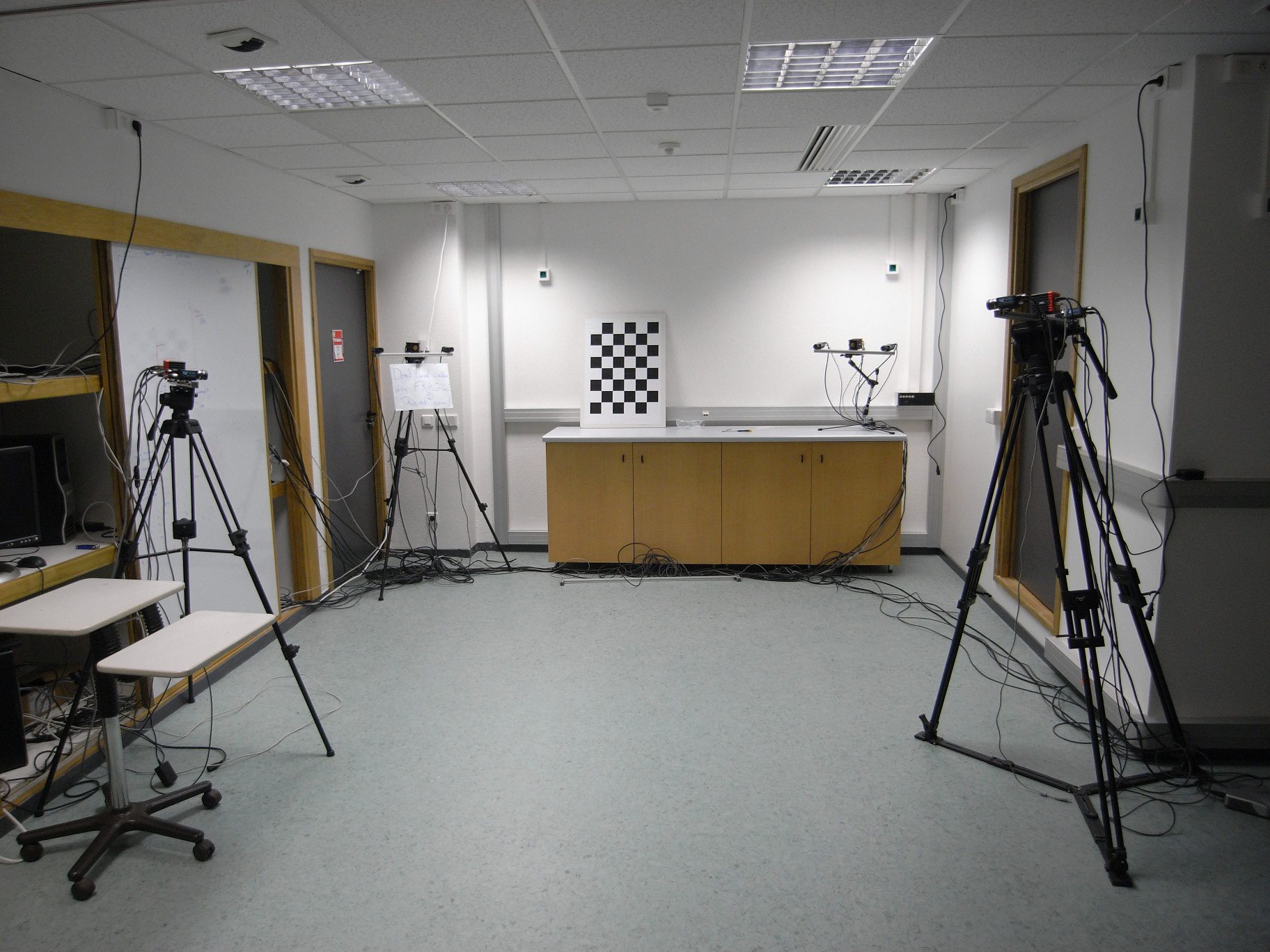
Figure 1: A single tof+2rgb system (left), comprising a time-of-flight camera in the centre, plus a pair of ordinary colour cameras. This paper addresses the problem of simultaneously cross-calibrating many such systems (right), as a foundation for scene understanding

1.2 Previous work

Multi-view depth and colour camera-networks, of the kind used here, produce data-streams that are subject to a variety of geometric relationships hartley-2000 . These relationships depend on the calibration state, relative orientation, and fields of view of the different cameras. It follows that a variety of calibration strategies can be adopted. These are discussed below, with reference to the literature, and contrasted with the approach presented here.

Perhaps the simplest way to combine rgb and tof data is to perform an essentially 2-d registration between the images and depth maps, as reviewed in nair-2013 ; see also huhle-2007 ; bartczak-2009 ; bleiweiss-2009 . This 2-d approach, however, can only provide an instantaneous solution, because changes in the scene-structure produce corresponding changes in the image-to-image mapping. Moreover, owing to the different viewpoints, a complete registration will usually be impossible. If the depth camera also produces a reliable intensity image, then photo-consistency can be used as a 3-d calibration criterion. For example, Beder et al. beder-2008 (see also schiller-2008 ; koch-2009 ) reproject the intensities of the depth data into the colour images, and optimize the camera parameters with respect to the photo-consistency.

Zhu et al. zhu-2011 (see also zhu-2008 ) present a sensor-fusion framework for the integration of tof depth and binocular disparity information. This method assumes that a dense disparity map is being computed on-line, which is not required by the method presented in this paper. Furthermore, the geometric calibration method zhu-2011 requires manual identification of corresponding points, and is based on a weak perspective camera model. In contrast, our method is automatic, and is based on the more appropriate perspective camera model. However, zhu-2011 is complementary to our method, in the sense that their sensor-fusion framework (along with a dense stereo-matcher) could be combined with the projective calibration method described below. Wang and Jia wang-2012 describe a related sensor-fusion framework for Kinect (rather than tof) depth data and colour images.

Another approach to the multi-modal calibration problem is to apply standard methods, as far as possible, to the depth cameras. Wu et al. wu-2009 describe an example of this approach. Lindner et al. lindner-2010 analyze the applicability of standard methods to tof cameras, as well as characterizing the accuracy of the depth data. Mure-Dubois and Hügli mure-2008 describe the Euclidean alignment of multiple tof point clouds, having calibrated the cameras by standard methods.

Silva et al. silva-2012 describe a cross-calibration methodology that is based on the identification of 3-d lines in the tof data, which are then projected to corresponding 2-d lines in the rgb images. This method does not require a chequerboard or other calibration pattern; it does, however, require the existence and detection of straight depth-edges throughout the scene. The approach of Silva et al. also involves a non-trivial correspondence problem, which in turn influences the calibration accuracy. Our method uses a standard chequerboard pattern, with a known number of vertices, for which the correspondence problem is relatively straightforward.

Zhang and Zhang zhang-2011 present cross-calibration methodology that is based on plane constraints, as given in zhang-1999 . This has the advantage of not requiring 2-d features to be detected in the (low resolution) tof images. However, this method cannot address the crucial issue of lens distortion, which is considerable in typical tof cameras kim-2008 . A related Kinect-based calibration system is described by Herrera et al. herrera-2012 , again using the plane-based method of zhang-1999 . Herrera et al. give a careful analysis of the Kinect intrinsic parameters, including lens and depth distortion. The latter is analyzed in more detail by Teichman et al. teichman-2013 . Our method does require features to be detected in the tof images, but this also makes it straightforward to estimate the lens parameters, using standard techniques.

Mikhelson et al. mikhelson-2013 describe an automatic method for registering a Euclidean point-cloud (obtained from a Kinect device) to its 2-d image-projections. This method, like ours, is based on a chequerboard target. However, Mikhelson et al. perform Euclidean 2-d/3-d registration, in contrast to the more general projective 3-d/3-d registration that is described below. Finally, there are methods that perform 3-d/3-d registration of dense data, subject to pointwise adjustments cui-2013 . This strategy can achieve very close registrations, but introduces a more complex optimization problem, which is not fully compatible with the standard calibration pipeline.

1.3 Paper organization and contributions

This paper is organized as follows. Section 2.1 briefly reviews some standard material on projective reconstruction, while section 2.2 describes the representation of range data in the present work. The chief contributions of the subsequent sections are as follows: Section 2.3 describes a point-based method that maps a classical multi-view reconstruction (projective or Euclidean) of the scene onto the corresponding tof representation. The data are obtained from a tof+2rgb system, as shown in figure 1. This does not require the colour cameras to be calibrated (although it is necessary to correct for lens distortion). It is established that this model includes a projective-linear approximation of the systematic tof depth-error.

Section 3 addresses the problem of multi-system alignment, which is necessary for complete scene-coverage. It is shown that this can be achieved in a way that is compatible with the individual tof+2rgb calibrations. The complete cross-calibration pipeline, given a collection of chequerboard images, is fully automatic.

Section 4 contains a detailed evaluation of these methods, using several large data-sets, captured by three tof+2rgb systems (i.e. a nine-camera network). In particular, section 4.1 extends the usual concepts of reprojection error hartley-2000 to the multi-modal case. Section 4.2 then introduces a new metric for mixed tof/rgb systems, which measures instantaneous sensor noise, as well as calibration error. The appropriateness of the 3-d homography transformation, as opposed to a similarity transformation, is tested in section 4.3. Section 4.4 discusses possible applications of these systems, including some real 3-d reconstruction examples. Conclusions and future directions are discussed in section 5.

The system presented here is based on the approach introduced by Hansard et al. hansard-2011 ; hansard-2013 . The earlier work has been improved, and extended to the case of multiple tof  and colour cameras. In addition, a new evaluation methodology has been developed, as described above. The automatic detection of calibration targets in the low-resolution tof images, which is a pre-requisite for the methods described here, was developed in a separate paper hansard-2014 .

2 Cross-calibration

This section describes the theory of projective alignment, using the following notation. Bold type will be used for vectors and matrices. In particular, points $\mathitbf{P}$, $\mathitbf{Q}$ and planes $\mathitbf{U}$, $\mathitbf{V}$ in the 3-d scene will be represented by column-vectors of homogeneous coordinates, e.g.

$$\mathitbf{P}=\begin{pmatrix}\mathitbf{P}_{\mspace{-1.0mu}\vartriangle}\\ P_{4}\end{pmatrix}\quad\text{and}\quad\mathitbf{U}=\begin{pmatrix}\mathitbf{U}_{\mspace{-1.0mu}\vartriangle}\\ U_{4}\end{pmatrix}$$ (1)

where $\mathitbf{P}_{\mspace{-1.0mu}\vartriangle}=(P_{1},\,P_{2},\,P_{3})^{\mspace{0.0mu}\scriptscriptstyle\top}$ and $\mathitbf{U}_{\mspace{-1.0mu}\vartriangle}=(U_{1},\,U_{2},\,U_{3})^{\mspace{0.0mu}\scriptscriptstyle\top}$. The homogeneous coordinates are defined up to a non-zero scaling; for example, $\mathitbf{P}\simeq(\mathitbf{P}_{\mspace{-1.0mu}\vartriangle}/P_{4},1)^{\mspace{0.0mu}\scriptscriptstyle\top}$. In particular, if $P_{4}=1$, then $\mathitbf{P}_{\mspace{-1.0mu}\vartriangle}$ contains the ordinary space coordinates of the point $\mathitbf{P}$. Furthermore, if $|\mathitbf{U}_{\mspace{-1.0mu}\vartriangle}|=1$, then $U_{4}$ is the signed perpendicular distance of the plane $\mathitbf{U}$ from the origin, and $\mathitbf{U}_{\mspace{-1.0mu}\vartriangle}$ is the unit normal. The point $\mathitbf{P}$ is on the plane $\mathitbf{U}$ if $\mathitbf{U}^{\mspace{0.0mu}\scriptscriptstyle\top}\mspace{-2.0mu}\mathitbf{P}=0$. The cross product $\mathitbf{u}\times\mathitbf{v}$ is often expressed as $(\mathitbf{u})_{\times}\mathitbf{v}$, where $(\mathitbf{u})_{\times}$ is a $3\times 3$ antisymmetric matrix. The column-vector of $N$ zeros is written $\mathitbf{0}_{N}$. Projective cameras are represented by $3\times 4$ matrices. For example, the range projection is

$$\mathitbf{q}\simeq\mathitbf{C}\mathitbf{Q}\quad\text{where}\quad\mathitbf{C}=\bigr{(}\mathitbf{A}_{3\times 3}\,|\,\mathitbf{b}_{3\times 1}\bigr{)}$$ (2)

is a block-decomposition of the $3\times 4$ camera matrix. The left and right colour cameras $\mathitbf{C}_{\ell}$ and $\mathitbf{C}_{r}$ are similarly defined, e.g. $\mathitbf{p}_{\ell}\simeq\mathitbf{C}_{\ell}\mathitbf{P}$. Table 1 summarizes the geometric objects that will be aligned.

	Observed	Reconstructed
	Points	Points	Planes
Binocular $\mathitbf{C}_{\ell}$,$\mathitbf{C}_{r}$	$\mathitbf{p}_{\ell}$, $\mathitbf{p}_{r}$	$\mathitbf{P}$	$\mathitbf{U}$
Range $\mathitbf{C}$	$(\mathitbf{q},\rho)$	$\mathitbf{Q}$	$\mathitbf{V}$

Table 1: Summary of notations in the left, right and range systems.

Points and planes in the two systems are related by the unknown $4\times 4$ space-homography $\mathitbf{H}$, so that

$$\mathitbf{Q}\simeq\mathitbf{H}\mathitbf{P}\quad\text{and}\quad\mathitbf{V}\simeq\mathitbf{H}^{-{\mspace{0.0mu}\scriptscriptstyle\top}}\mspace{-3.0mu}\mathitbf{U}.$$ (3)

This model encompasses all rigid, similarity and affine transformations in 3-d. It preserves collinearity and flatness, and is linear in homogeneous coordinates. Note that, in the reprojection process, $\mathitbf{H}$ can be interpreted as a modification of the camera matrices. For example, $\mathitbf{p}_{\ell}\simeq\bigl{(}\mathitbf{C}_{\ell}\mathitbf{H}^{-1}\bigr{)}\mathitbf{Q}$, where $\mathitbf{H}^{-1}\mathitbf{Q}\simeq\mathitbf{P}$ is the point that would theoretically be reconstructed by triangulation.

The $4\times 4$ homographies $\mathitbf{H}$ include, as special cases, the rigid transformations that would align a fully-calibrated Euclidean stereo-reconstruction to the tof measurements. There are two motivations for the generalization. Firstly, it allows uncalibrated binocular reconstructions to be used, as described above. Secondly, it has been shown elsewhere kolb-2010 ; zhu-2011 that tof data are subject to systematic depth biases and nonlinear distortions. These are difficult to correct, owing to the lack of a complete parametric model, and to their dependence on the camera settings (e.g. integration time). Nonetheless, the homography model (3) effectively includes a projective-linear approximation of the depth distortion, which is fitted along with the other transformation parameters. This model is quite powerful: it includes rational depth-distortions, with varying parameters, across each bundle of rays. For example, the two-parameter inverse disparity calibration, as used with Kinect devices herrera-2012 , is a special case of the homography model described here. Indeed, even if the rgb cameras are fully calibrated, the 3-d homographies are needed to account for depth-distortions and residual reconstruction errors, as demonstrated in hansard-2011 . This issue will be explored in section 4.3, below.

2.1 Parallax-based reconstruction

A projective reconstruction of the scene can be obtained from matched points $\mathitbf{p}_{\ell k}$ and $\mathitbf{p}_{rk}$, together with the fundamental matrix $\mathitbf{F}$, where $\mathitbf{p}_{rk}^{\mspace{0.0mu}\scriptscriptstyle\top}\mathitbf{F}\,\mathitbf{p}_{\ell k}=0$. The fundamental matrix can be estimated automatically, using the well-established ransac method. The camera matrices can then be determined, up to a four-parameter projective ambiguity hartley-2000 . In particular, from $\mathitbf{F}$ and the epipole $\mathitbf{e}_{r}$, the cameras can be defined as

$$\mathitbf{C}_{\ell}\simeq\bigl{(}\mathitbf{I}\,|\,\mathitbf{0}_{3})\hskip 6.00006pt\text{and}\hskip 5.0pt\mathitbf{C}_{r}\simeq\bigl{(}(\mathitbf{e}_{r})_{\times}\mathitbf{F}+\mathitbf{e}_{r}\mathitbf{g}^{\mspace{0.0mu}\scriptscriptstyle\top}\,\big{|}\,\gamma\mathitbf{e}_{r}\bigr{)}.$$ (4)

where $\gamma\neq 0$ and $\mathitbf{g}=(g_{1},\,g_{2},\,g_{3})^{\mspace{0.0mu}\scriptscriptstyle\top}$ can be used to bring the cameras into a plausible form. This makes it easier to visualize the projective reconstruction and, more importantly, can improve the numerical conditioning of subsequent procedures.

2.2 Range-based reconstruction

The tof camera $\mathitbf{C}$ provides the range (i.e. radial distance) $\rho$ of each scene-point from the camera-centre, as well as the associated image-coordinates $\mathitbf{q}=(x,y,1)$. The back-projection of this point into the scene is

$$\mathitbf{Q}_{\mspace{-1.0mu}\vartriangle}=\mathitbf{A}^{-1}\bigl{(}(\rho/\alpha)\,\mathitbf{q}-\mathitbf{b}\bigr{)}\quad\text{where}\quad\alpha=\bigl{|}\mathitbf{A}^{-1}\,\mathitbf{q}\bigr{|}.$$ (5)

Hence the point $(\mathitbf{Q}_{\mspace{-1.0mu}\vartriangle},1)^{\mspace{0.0mu}\scriptscriptstyle\top}$ is at distance $\rho$ from the optical centre $-\mathitbf{A}^{-1}\mathitbf{b}$, in the direction $\mathitbf{A}^{-1}\mathitbf{q}$. The scalar $\alpha$ serves to normalize the direction-vector. This is the standard pinhole model, as used in beder-2007 .

The range data are noisy and incomplete, owing to illumination and scattering effects. This means that, given a sparse set of features in the intensity image (of the tof device), it is not advisable to use the back-projected point (5) directly. A better approach is to segment the image of the plane in each tof camera (using the the range and/or intensity data). It is then possible to back-project all of the enclosed points, and to robustly fit a plane $\mathitbf{V}_{j}$ to the enclosed points $\mathitbf{Q}_{ij}$, so that $\mathitbf{V}_{j}^{\mspace{0.0mu}\scriptscriptstyle\top}\!\mathitbf{Q}_{ij}\approx 0$ if point $i$ lies on plane $j$. Now, the back-projection $\mathitbf{Q}_{\pi}$ of each sparse feature point $\mathitbf{q}$ can be obtained by intersecting the corresponding ray with the plane $\mathitbf{V}$, so that the new range estimate $\rho^{\pi}$ is

$$\rho^{\pi}=\frac{\mathitbf{V}_{\mspace{-1.0mu}\vartriangle}^{\mspace{0.0mu}\scriptscriptstyle\top}\mathitbf{A}^{-1}\mathitbf{b}-V_{4}}{(1/\alpha)\,\mathitbf{V}_{\mspace{-1.0mu}\vartriangle}^{\mspace{0.0mu}\scriptscriptstyle\top}\mathitbf{A}^{-1}\mathitbf{q}}$$ (6)

where $|V_{4}|$ is the distance of the plane to the camera centre, and $\mathitbf{V}_{\mspace{-1.0mu}\vartriangle}$ is the unit-normal of the range plane. The new point $\mathitbf{Q}^{\pi}$ is obtained by substituting $\rho^{\pi}$ into (5).

The choice of plane-fitting method is affected by two issues. Firstly, there may be very severe outliers in the data, due to the photometric and geometric errors in the depth-estimation process. Secondly, the noise-model should be based on the pinhole geometry, which means that perturbations occur radially along visual directions, which are not (in general) perpendicular to the observed plane hebert-1992 ; wang-2001 . Several plane-fitting methods, both iterative kanazawa-1995 and non-iterative pathak-2009 have been proposed for the pinhole model. However, for tof data, the chief problem is the large number of outliers. This means that a ransac-based method is the most effective in this context hansard-2011 .

2.3 Projective Alignment

It is straightforward to show that the transformation $\mathitbf{H}$ in (3) could be estimated from five binocular points $\mathitbf{P}_{k}$, together with the corresponding range points $\mathitbf{Q}_{k}$. This would provide $5\times 3$ equations, which determine the $4\times 4$ entries of $\mathitbf{H}$, subject to an overall projective scaling. It is better, however, to use the ‘Direct Linear Transformation’ method hartley-2000 , which fits $\mathitbf{H}$ to all of the data. This method is based on the fact that if

$$\mathitbf{P}^{\prime}=\mathitbf{H}\mathitbf{P}$$ (7)

is a perfect match for $\mathitbf{Q}$, then $\mu\mathitbf{Q}=\lambda\mathitbf{P}^{\prime}$, and the scalars $\lambda$ and $\mu$ can be eliminated between pairs of the four implied equations csurka-1999 . This results in $\binom{4}{2}=6$ interdependent constraints per point. It is convenient to write these homogeneous equations as

$$\begin{pmatrix}Q_{4}\mathitbf{P}_{\mspace{-1.0mu}\vartriangle}^{\prime}-P_{4}^{\prime}\mspace{1.0mu}\mathitbf{Q}_{\mspace{-1.0mu}\vartriangle}\\[4.30554pt] \mathitbf{Q}_{\mspace{-1.0mu}\vartriangle}\times\mathitbf{P}_{\mspace{-1.0mu}\vartriangle}^{\prime}\end{pmatrix}=\mathitbf{0}_{\mspace{2.0mu}6}.$$ (8)

Note that if $\mathitbf{P}^{\prime}$ and $\mathitbf{Q}$ are normalized so that $P^{\prime}_{4}=1$ and $Q_{4}=1$, then the magnitude of the top half of (8) is simply the distance between the points. Following Förstner forstner-2005 , the left-hand side of (8) can be expressed as $\bigl{(}\mathitbf{Q}\bigr{)}_{\wedge}\mathitbf{P}^{\prime}$ where

$$\bigl{(}\mathitbf{Q}\bigr{)}_{\wedge}=\begin{pmatrix}Q_{4}\mathitbf{I}_{3}&-\mathitbf{Q}_{\mspace{-1.0mu}\vartriangle}\\[4.30554pt] \bigl{(}\mathitbf{Q}_{\mspace{-1.0mu}\vartriangle}\bigr{)}_{\times}&\mathitbf{0}_{\mspace{2.0mu}3}\end{pmatrix}$$ (9)

is a $6\times 4$ matrix, and $\bigl{(}\mathitbf{Q}_{\mspace{-1.0mu}\vartriangle}\bigr{)}_{\times}\mathitbf{P}_{\mspace{-1.0mu}\vartriangle}=\mathitbf{Q}_{\mspace{-1.0mu}\vartriangle}\times\mathitbf{P}_{\mspace{-1.0mu}\vartriangle}$, as usual. The equations (8) can now be written in terms of (7) and (9) as

$$\bigl{(}\mathitbf{Q}\bigr{)}_{\wedge}\mathitbf{H}\mathitbf{P}=\mathitbf{0}_{\mspace{2.0mu}6}.$$ (10)

This system of equations is linear in the unknown entries of $\mathitbf{H}$, the columns of which can be stacked into the $16\times 1$ vector $\mathitbf{h}$. The Kronecker product identity $\mathrm{vec}(\mathitbf{X}\,\mathitbf{Y}\,\mathitbf{Z})=$ $(\mathitbf{Z}^{\mspace{0.0mu}\scriptscriptstyle\top}\!\otimes\mathitbf{X})\,\mathrm{vec}(\mathitbf{Y})$ can now be applied, to give

$$\Bigl{(}\mathitbf{P}^{\mspace{0.0mu}\scriptscriptstyle\top}\otimes\bigl{(}\mathitbf{Q}\bigr{)}_{\wedge}\Bigr{)}\mathitbf{h}=\mathitbf{0}_{\mspace{2.0mu}6}\quad\text{where}\quad\mathitbf{h}=\mathrm{vec}\bigl{(}\mathitbf{H}\bigr{)}.$$ (11)

If $M$ points are observed on each of $N$ planes, then there are $k=1,\ldots,MN$ observed pairs of points, $\mathitbf{P}_{k}$ from the projective reconstruction and $\mathitbf{Q}_{k}$ from the range back-projection. The $MN$ corresponding $6\times 16$ matrices $\bigl{(}\mathitbf{P}_{k}^{\mspace{0.0mu}\scriptscriptstyle\top}\otimes(\mathitbf{Q}_{k})_{\wedge}\bigr{)}$ are stacked together, to give the complete system

$$\begin{pmatrix}\mathitbf{P}_{1}^{\mspace{0.0mu}\scriptscriptstyle\top}&\otimes&\bigl{(}\mathitbf{Q}_{1}\bigr{)}_{\wedge}\\ &\vdots&\\ \mathitbf{P}_{MN}^{\mspace{0.0mu}\scriptscriptstyle\top}&\otimes&\bigl{(}\mathitbf{Q}_{MN}\bigr{)}_{\wedge}\end{pmatrix}\mathitbf{h}=\mathitbf{0}_{\mspace{2.0mu}6MN}$$ (12)

subject to the constraint $|\mathitbf{h}|=1$, which excludes the trivial solution $\mathitbf{h}=\mathitbf{0}_{16}$. It is straightforward to obtain an estimate of $\mathitbf{h}$ from the SVD of the the $6MN\times 16$ matrix on the left of (12). This solution, which minimizes an algebraic error hartley-2000 , is the singular vector corresponding to the smallest singular value of the matrix. Note that the point coordinates should be transformed, to ensure that (12) is numerically well-conditioned hartley-2000 . In this case the transformation ensures that $\sum_{k}\mathitbf{P}_{k{\mspace{-1.0mu}\vartriangle}}=\mathitbf{0}_{3}$ and $\frac{1}{MN}\sum_{k}|\mathitbf{P}_{k{\mspace{-1.0mu}\vartriangle}}|=\sqrt{3}$, where $P_{k4}=1$. The analogous transformation is applied to the range points $\mathitbf{Q}_{k}$.

The above procedure effectively computes a projective basis in 3-d, which requires five points, no four of which may be co-planar. This gives $5\times 3$ numbers, which are equivalent to the 15 parameters of the homogeneous $4\times 4$ matrix $\mathitbf{H}$. In practice, however, we require full detection of 35 vertices per board, and around 10 boards per homography (depending on visibility constraints). Hence the procedure operates far from any degenerate cases, which would involve fewer than 15 degrees of freedom in total.

The DLT method, in practice, gives a good approximation $\mathitbf{H}_{\scriptscriptstyle\mathrm{DLT}}$ of the homography (3). This can be used as a starting-point for the iterative minimization of a more appropriate error measure. In particular, consider the reprojection error in the left image,

$$E_{\ell}(\mathitbf{C}_{\ell})=\sum_{k=1}^{MN}D\bigl{(}\mathitbf{C}_{\ell}\mathitbf{Q}_{k},\,\mathitbf{p}_{\ell k}\bigr{)}^{2}$$ (13)

where $D(\mathitbf{p},\mathitbf{q})=|\,\mathitbf{p}_{\mspace{-1.0mu}\vartriangle}/p_{3}-\mathitbf{q}_{\mspace{-1.0mu}\vartriangle}/q_{3}|$. A $12$-parameter minimization of the reprojection error (13), starting with the linear estimate $\mathitbf{C}_{\ell}\leftarrow\mathitbf{C}_{\ell}\mathitbf{H}_{\scriptscriptstyle\mathrm{DLT}}^{-1}$, is then performed by the Levenberg-Marquardt algorithm press-1992 . The result will be the camera matrix $\mathitbf{C}_{\ell}^{\star}$ that best reprojects the range data into the left image ($\mathitbf{C}_{r}^{\star}$ is similarly obtained). The solution, provided that the calibration points adequately covered the scene volume, will remain valid for subsequent depth and range data.

Alternatively, it is possible to minimize the joint reprojection error, defined as the sum of left and right contributions,

$$E\bigl{(}\mathitbf{H}^{-1}\bigr{)}=E_{\ell}\bigl{(}\mathitbf{C}_{\ell}\mathitbf{H}^{-1}\bigr{)}+E_{r}\bigl{(}\mathitbf{C}_{r}\mathitbf{H}^{-1}\bigr{)}$$ (14)

over the (inverse) homography $\mathitbf{H}^{-1}$. The 16 parameters are again minimized by the Levenberg-Marquardt algorithm, starting from the DLT solution $\mathitbf{H}_{\scriptscriptstyle\mathrm{DLT}}^{-1}$.

The difference between the separate (13) and joint (14) minimizations is that the latter preserves the original epipolar geometry, whereas the former does not. Recall that $\mathitbf{C}_{\ell}$ $\mathitbf{C}_{r}$, $\mathitbf{H}$ and $\mathitbf{F}$ are all defined up to scale, and that $\mathitbf{F}$ satisfies an additional rank-two constraint hartley-2000 . Hence the underlying parameters can be counted as $(12-1)+(12-1)=22$ in the separate minimizations, and as $(16-1)=15$ in the joint minimization. The fixed epipolar geometry accounts for the $(9-2)$ missing parameters in the joint minimization. If $\mathitbf{F}$ is known to be very accurate (or must be preserved) then the joint minimization (14) should be performed. This will also preserve the original binocular triangulation, provided that a projective-invariant method was used hartley-1997 . However, if minimal reprojection error is the objective, then the cameras should be treated separately. This will lead to a new fundamental matrix $\mathitbf{F}^{\star}=(\mathitbf{e}_{r}^{\star})_{\times}\mathitbf{C}_{r}^{\star}(\mathitbf{C}_{\ell}^{\star})^{+}$, where $(\cdot)^{+}$ is the generalized inverse, and $\mathitbf{C}_{\ell}^{\star}$, $\mathitbf{C}_{r}^{\star}$ are the optimized camera-matrices. The epipole in the right-hand image is obtained from $\mathitbf{e}_{r}^{\star}=\mathitbf{C}_{r}^{\star}\mathitbf{d}_{\ell}^{\star}$, where the vector $\mathitbf{d}_{\ell}^{\star}$ represents the nullspace $\mathitbf{C}_{\ell}^{\star}\mathitbf{d}_{\ell}^{\star}=\mathitbf{0}_{3}$.

3 Multi-System Alignment

The methods described in section 2.3 can be used to calibrate a single tof+2rgb system; the joint calibration of several such systems will now be explained. In this section the notation $\mathitbf{P}_{i}$ will be used for the binocular coordinates (with respect to the left camera) of a point in the $i$-th system, and likewise $\mathitbf{Q}_{i}$ for the tof coordinates of a point in the same system. Hence the $i$-th tof, left and right rgb cameras (sharing the same physical mounting) have the form

$$\begin{gathered}\mathitbf{C}_{i}\simeq\bigl{(}\mathitbf{A}_{i}\,|\,\mathitbf{0}_{3})\\ \mathitbf{C}_{\ell i}\simeq\bigl{(}\mathitbf{A}_{\ell i}\,|\,\mathitbf{0}_{3})\quad\text{and}\quad\mathitbf{C}_{ri}\simeq\bigl{(}\mathitbf{A}_{ri}\,|\,\mathitbf{b}_{ri})\end{gathered}$$ (15)

where $\mathitbf{A}_{i}$ and $\mathitbf{A}_{\ell i}$ contain only intrinsic parameters, whereas $\mathitbf{A}_{ri}$ also encodes the relative orientation of $\mathitbf{C}_{ri}$ with respect to $\mathitbf{C}_{\ell i}$. Each system has a transformation $\mathitbf{H}_{i}^{-1}$ that maps tof points $\mathitbf{Q}_{i}$ into the corresponding rgb coordinate system of $\mathitbf{C}_{\ell i}$. Furthermore, let the $4\times 4$ matrix $\mathitbf{G}_{ij}$ be the transformation from system $j$, mapping back to system $i$ (between different physical mountings). This matrix, in the binocularly-calibrated case, is a rigid 3-d transformation. However, by analogy with the tof-to-rgb matrices $\mathitbf{H}$, each $\mathitbf{G}_{ij}$ could be a projective transformation in the uncalibrated case; this would allow Euclidean structure to propagate from the tof measurements, across the entire camera network.

The left and right cameras, in all cases, that project a scene-point $\mathitbf{P}_{\!j}$ in coordinate system $j$ to image-points $\mathitbf{p}_{\ell i}$ and $\mathitbf{p}_{ri}$ in system $i$ are

$$\mathitbf{C}_{\ell ij}=\mathitbf{C}_{\ell i}\,\,\mathitbf{G}_{ij}\quad\text{and}\quad\mathitbf{C}_{rij}=\mathitbf{C}_{ri}\,\,\mathitbf{G}_{ij}.$$ (16)

Note that if a single global coordinate system is chosen to coincide with the $k$-th rgb system, then a point $\mathitbf{P}_{k}$ projects via $\mathitbf{C}_{\ell ik}$ and $\mathitbf{C}_{rik}$. These two cameras are respectively equal to $\mathitbf{C}_{\ell i}$ and $\mathitbf{C}_{ri}$ in (15) only when $i=k$, such that $\mathitbf{G}_{ij}=\mathitbf{I}$ in (16). A typical three-system configuration is shown in fig. 2.

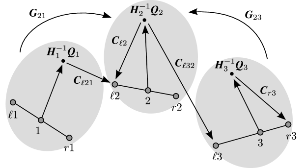
Figure 2: Example of a three tof+2rgb setup, with tof cameras labelled 1,2,3; cf. fig. 1. Each ellipse represents a separate system, with system 2 chosen as the reference. The arrows (with camera-labels) show some possible tof-to-rgb projections. For example, a point $\mathitbf{P}_{2}\simeq\mathitbf{H}_{2}^{-1}\mathitbf{Q}_{2}$ in the centre projects directly to rgb view $\ell 2$ via $\mathitbf{C}_{\ell 2}$, whereas the same point projects to $\ell 3$ via $\mathitbf{C}_{\ell 32}=\mathitbf{C}_{\ell 3}\mathitbf{G}_{32}$.

The transformation $\mathitbf{G}_{ij}$ can only be estimated directly if there is a region of common visibility between systems $i$ and $j$. If this is not the case (as when the systems face each other, such that the front of the calibration board is not simultaneously visible), then $\mathitbf{G}_{ij}$ can be computed indirectly. For example, $\mathitbf{G}_{02}=\mathitbf{G}_{01}\,\mathitbf{G}_{12}$ where $\mathitbf{P}_{2}=\mathitbf{G}_{12}^{-1}\mathitbf{G}_{01}^{-1}\mathitbf{P}_{0}$. Note that, in all cases, the stereo-reconstructed points $\mathitbf{P}$ are used to estimate these transformations This is because they are always more reliable than the tof points $\mathitbf{Q}$, as demonstrated below.

4 Evaluation

The following sections will describe the accuracy of a nine-camera setup, calibrated by the methods described above. Section 4.1 will evaluate calibration error, whereas section 4.2 will evaluate total error. The former is essentially a fixed function of the estimated camera matrices, for a given scene. The latter also includes the range-noise from the tof cameras, which varies from moment to moment (due to intrinsic noise, changing illumination, and object motion). The importance of this distinction will be discussed. In section 4.3 we analyze the avantages of using homographies to align the data, as opposed to similarity transformations. Finally, in section 4.4 we demonstrate some applications of the complete system.

The setup consists of three rail-mounted tof+2rgb systems, $i=1\ldots 3$, as in fig. 2. The stereo baselines are 17cm on average, and the tof cameras are separated by 107cm on average. The rgb images are $1624\times 1224$, whereas the Mesa Imaging sr4000 tof images are $176\times 144$, with a depth range of 500cm mesa-2010 . The three stereo systems are first calibrated by standard methods hartley-2000 , returning a full Euclidean decomposition of $\mathitbf{C}_{\ell i}$ and $\mathitbf{C}_{ri}$, as well as the associated lens parameters. The lenses of the tof cameras are also calibrated by standard methods hartley-2000 . This removes some of the radial depth deformation that has been observed in the tof data cui-2013 . The matrices $\mathitbf{G}_{ij}$ are rigid-body transformations, which are estimated by the SVD method of Arun et al. arun-1987 . Projective alignment is preferred for the tof/rgb alignment, for reasons discussed in sections 2 and 10. Hence the transformations $\mathitbf{H}_{j}^{-1}$ are $4\times 4$ homographies, estimated by the method of section 2.3. Specifically, the DLT solutions were refined by Levenberg-Marquardt minimization of the joint geometric error, as in (14).

4.1 Calibration Error

The calibration error is measured by first taking tof points $\mathitbf{Q}^{\pi}_{j}$ corresponding to chequerboard vertices on the reconstructed calibration plane $\pi_{j}$ in system $j$, as described in section 2.2. These can then be projected into a pair of rgb images in system $i$, so that the geometric image-error $E^{\mathrm{cal}}_{ij}=\frac{1}{2}\bigl{(}E^{\mathrm{cal}}_{\ell ij}+E^{\mathrm{cal}}_{rij}\bigr{)}$ can be computed, where

$$E^{\mathrm{cal}}_{\ell ij}=\frac{1}{|\pi|}\sum_{\mathitbf{Q}_{j}^{\pi}}D\Bigl{(}\mathitbf{C}_{\ell ij}\,\mathitbf{H}_{j}^{-1}\mathitbf{Q}_{j}^{\pi},\,\,\,\mathitbf{p}_{\ell i}\Bigr{)}$$ (17)

and $E^{\mathrm{cal}}_{rij}$ is similarly defined. The function $D(\cdot,\cdot)$ computes the image-distance between two inhomogenized points, as in (13), and the denominator corresponds to the number of vertices on the board, with $|\pi|=35$ in the present experiments. The measure (17) can of course be averaged over all images in which the board is visible. The rgb cameras were calibrated, by standard methods, as described above. Subpixel accuracy was obtained, which confirms the accuracy of the camera matrices $\mathitbf{C}_{\ell i}$ and $\mathitbf{C}_{ri}$, as well as the inter-system matrices $\mathitbf{G}_{ij}$, where $i,j=1,2,3$.

For the purpose of evaluation, a new set of tof-vertices $\mathitbf{Q}^{\pi}_{i}$ were reconstructed, fitted and reprojected within each system $i$. This evaluation effectively tests the quality of the $\mathitbf{H}_{i}^{-1}$ matrices, by comparing $\mathitbf{C}_{\ell i}\mathitbf{H}_{i}^{-1}\mathitbf{Q}^{\pi}_{i}$ to $\mathitbf{p}_{\ell i}$, and analogously to points $\mathitbf{p}_{ri}$ in the other image. Note that all camera and transformations parameters are now fixed; no optimization was performed with respect to the evaluation data. The whole experiment was performed on three large data-sets, from different capture-sessions, and with different camera configurations, labelled A, B and C. Such a configuration leads to one triplet per system as shown in fig. 3. While an image can be fronto-parallel for one frame, it may appear very slanted to the other frames. The example of fig. 3 shows a calibration image that is almost fronto-parallel to the tof frame of the central tof+2rgb unit. Table 2 shows that the average reprojection error remains subpixel in all three data-sets. The corresponding error-distributions are shown as histograms in fig. 4.

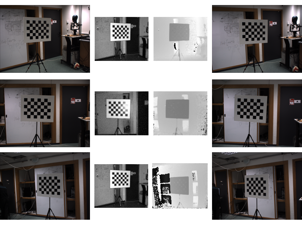
Figure 3: Calibration images from synchronized captures. Each row corresponds to the image triplet of a tof+2rgb system, while the range images are shown as well. Grayscale images of tof sensors have undergone lens undistortion and contrast enhancement.

Set	Mean	Median	Max	Count
A	0.59	0.52	1.82	1470
B	0.72	0.58	4.86	1470
C	0.45	0.40	1.48	1470

Table 2: Calibration error (17), measured by projecting the fitted tof vertices $\mathitbf{Q}^{\pi}_{i}$ to the left and right rgb images ($1624\times 1224$) of the respective systems $i=1,2,3$. The experiment was repeated three times (A–C), with different camera configurations. Each statistic was computed from the left and right rgb-reprojections of 35 vertices in 7 views of the board (total number of 2-d points, per data-set: $3\times 2\times 35\times 7=1470$).

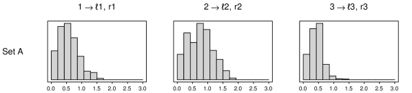
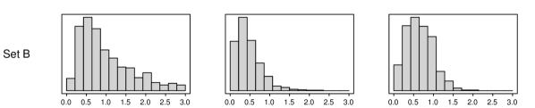
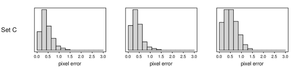
Figure 4: Calibration error (17), measured by projecting the fitted tof points $\mathitbf{Q}^{\pi}_{i}$ to the left and right rgb images ($1624\times 1224$) of the respective systems $i=1,2,3$. The experiment was repeated three times (A–C), with different camera configurations. Each histogram contains 1470 points, as in table 2.

It is also interesting to consider how the above tof-vertices reproject into different systems. The error 3-d error distribution, for a given pixel (either tof or stereo) is highly anisotropic; the direction of the corresponding ray is much more reliable than the distance along it cui-2013 . In practice, the different tof+2rgb systems are distributed around the edge of the room, looking inwards. Hence a given system is likely to be seen ‘from the side’ by at least one other system. This means that any large depth errors in the first system will not cancel-out in the re-projection to the other systems. This effect is seen clearly in figure 5, which shows calibration errors of up to several pixels, from one system to the others.

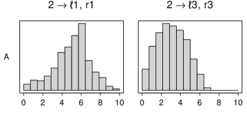
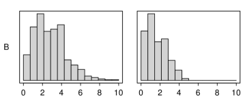
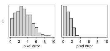
Figure 5: Calibration error (17), measured by projecting the fitted tof points $\mathitbf{Q}^{\pi}_{2}$ to the left and right rgb images ($1624\times 1224$) of two different systems, $i=1,3$. Each histogram combines left-camera and right-camera measurements from 7 views of the calibration board.

4.2 Total Error

The calibration error, as reported in the preceding section, is the natural way to evaluate the estimated cameras and homographies. It is not, however, truly representative of the ‘live’ performance of the complete setup. This is because the calibration error uses each estimated plane $\pi_{j}$ to replace all vertices $\mathitbf{Q}_{j}$ with the fitted versions $\mathitbf{Q}_{j}^{\pi}$. In general, however, no surface model is available, and so the raw points $\mathitbf{Q}_{j}$ must be used as input to segmentation, meshing and rendering processes.

The total error, which combines the calibration and range errors, can be measured as follows. The $i$-th rgb views of plane $\pi_{j}$ are related to the tof image-points $\mathitbf{q}_{j}$ by the 2-d transfer homographies $\mathitbf{T}_{\ell ij}$ and $\mathitbf{T}_{rij}$, where

$$\mathitbf{p}_{\ell i}\simeq\mathitbf{T}_{\ell ij}\,\mathitbf{q}_{j}\quad\text{and}\quad\mathitbf{p}_{ri}\simeq\mathitbf{T}_{rij}\,\mathitbf{q}_{j}.$$ (18)

These $3\times 3$ matrices can be estimated to subpixel accuracy, by using the DLT algorithm hartley-2000 to obtain initial homographies, and then applying area-based alignment Evangelidis2008 to produce the final estimates $\mathitbf{T}_{\ell ij}$ and $\mathitbf{T}_{rij}$.

Let $\Pi_{j}$ be the 2-d hull (i.e. bounding-polygon) of plane $\pi_{j}$ as it appears in the tof image. Any pixel $\mathitbf{q}_{j}$ in the hull (including the original calibration vertices) can now be re-projected to the $i$-th rgb views via the 3-d point $\mathitbf{Q}_{j}$, or transferred directly by $\mathitbf{T}_{\ell ij}$ and $\mathitbf{T}_{rij}$ in (18), as shown in figure 6. In other words, we are able to isolate the image-to-image error that is incurred by mapping via the 3-d reconstruction, in relation to the direct 2-d to 2-d mapping defined by $\mathitbf{T}_{\ell ij}$ and $\mathitbf{T}_{rij}$.

The total error is the average difference between the reprojections and the transfers, $E^{\mathrm{tot}}_{ij}=\frac{1}{2}\bigl{(}E^{\mathrm{tot}}_{\ell ij}+E^{\mathrm{tot}}_{rij}\bigr{)}$, where

$$E^{\mathrm{tot}}_{\ell ij}=\frac{1}{|\Pi_{j}|}\sum_{\mathitbf{q}_{j}\in\Pi_{j}}D\Bigl{(}\mathitbf{C}_{\ell ij}\,\mathitbf{H}_{j}^{-1}\mathitbf{Q}_{j},\,\,\,\mathitbf{T}_{\ell ij}\,\mathitbf{q}_{j}\Bigr{)}$$ (19)

and $E^{\mathrm{tot}}_{rij}$ is similarly defined. The view-dependent denominator $|\Pi_{j}|\gg|\pi|$ is the number of pixels in the hull $\Pi_{j}$. Hence $E^{\mathrm{tot}}_{ij}$ is the total error, including both calibration errors and range-noise, of tof plane $\pi_{j}$ as it appears in the $i$-th rgb cameras.

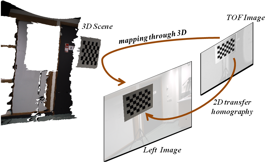
Figure 6: The 2-d transfer homography $\mathitbf{T}_{\ell}$ describes the chessboard mapping from the tof frame to the left frame. In principle, this mapping should be equivalent to a mapping via the range data, i.e. from the tof frame to the measured 3-d plane, and back to the left frame.

If the rgb cameras are not too far from the tof camera, then the range errors tend to be cancelled in the reprojection. This is evident from table 3, in which the total errors, on average, are not much greater than the calibration errors in table 2. It is, however, clear from fig. 7, that the tails of the total error distributions are greatly increased by outliers in the tof data-stream. Although errors up to $3$ pixels are shown in distributions for the sake of clarity, maximum errors of more than five pixels are common (see table 3).

Set	Mean	Median	Max	Count
A	0.74	0.71	6.07	39859
B	1.48	0.98	20.69	32159
C	0.63	0.54	6.51	29442

Table 3: Total error (19), measured by projecting the raw tof points $\mathitbf{Q}_{i}$ to the left and right rgb images ($1624\times 1224$) of the respective systems $i=1,2,3$. These figures characterize the raw data that is produced by the live system. This data includes all outliers in the tof data-stream, which gives rise to at least one error of 20 pixels here.

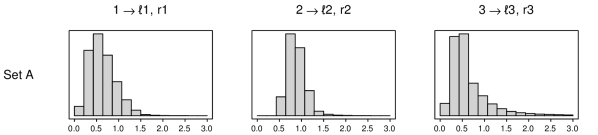
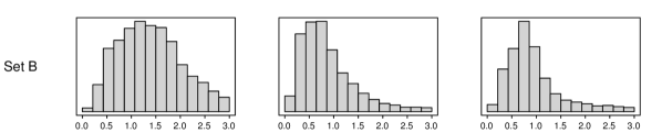
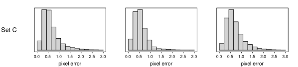
Figure 7: Total error (19), measured by projecting the raw tof points $\mathitbf{Q}_{i}$ to the left and right rgb images ($1624\times 1224$) of the respective systems $i=1,2,3$. These distributions have longer and heavier tails than those of the corresponding calibration errors, shown in fig. 4.

When the raw tof points are reprojected to a different system, a high total error is expected, because the sensor’s range-noise may be viewed ‘from the side’. Indeed, fig. 8 shows that a substantial proportion of the tof points reproject with total errors in excess of ten pixels. These kind of gross errors are characteristic of the tof data, owing to the inevitable presence of absorbing and scattering surfaces in a typical scene.

In fact, calibration error and total error are both influenced by surface orientation. For example, the higher errors in Set B of the data (see tables 2 and 3) are due to the presence of some very slanted boards, in both the fitting and evaluation data-sets; this causes two problems, as follows. Firstly, the images of these boards are very foreshortened in some systems. This leads to increased calibration error, because the vertices are hard to detect in the corresponding tof images. Secondly, the strength of the reflected IR signal is reduced whenever the surface is oblique to a given tof camera. If the surface is also absorbent (like the black squares of the board), then the total error is greatly increased, due to the combined effects of scattering and absorption.

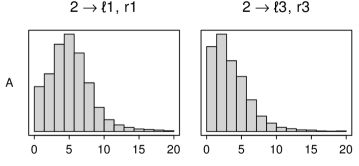
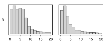
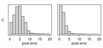
Figure 8: Total error (19), measured by projecting the fitted tof points $\mathitbf{Q}^{\pi}_{2}$ to the left and right rgb images ($1624\times 1224$) of two different systems, $i=1,3$. The range errors are emphasized by the difference in viewpoints between the two systems. Average error is now around five pixels, and the noisiest tof points reproject with tens of pixels of error.

It is possible to understand these results more fully by examining the distribution of the total error across individual boards. Figure 9 shows the distribution for a board reprojected to same/different systems (i.e. part of the data from figs. 7 & 8). There is a relatively smooth gradient of error across the board, which is attributable to errors in the fitting of plane $\pi_{j}$, and in the estimation of the camera parameters. In addition to these effects, it is clear that the gross errors are correlated with the black squares of the board, which reflect too little of the tof signal. For instance, in the bottom example of figure  9, the mean reprojection error associated with the black squares is $10.05$ pixels, whereas the white squares are associated with a mean error of $3.55$ pixels. The effect is particularly noticeable, as expected from the histograms, when reprojecting to different camera systems.

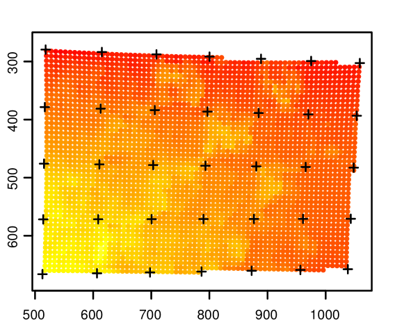
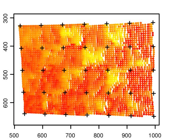
Figure 9: 3-d tof pixels on an example calibration board, projected into an RGB camera in the same (top) and in a different (bottom) system. Each pixel is colour-coded according to the relative total-error (19) in each case (larger errors are shown in yellow). Black crosses mark the detected vertices in the rgb image. The black squares of the board are associated with larger reprojection errors, particularly after reprojecting to a different system (mean error in the bottom example is 10.05px for black squares, and 3.55px for white).

4.3 Comparison of homography and similarity transformations

It was argued in section 2 that the 3-d homography model is an appropriate way to compensate for miscalibrations of the tof and stereo systems (and indeed it allows the stereo system to be left uncalibrated, if preferred hansard-2011 ). This claim is tested in the following experiments, using data images from two new data sets.

The most obvious alternative to the homography is a rigid motion and scaling; i.e. a 3-d similarity transformation. Specifically, the $4\times 4$ matrix $\mathitbf{H}$ in (3) can be replaced by the similarity transformation

$$\mathitbf{S}=\begin{pmatrix}\sigma\,\mathitbf{R}&\mathitbf{t}\\ \mathitbf{0}&1\end{pmatrix}$$ (20)

where $\sigma$ is a (positive) scalar, $\mathitbf{R}$ is a $3\times 3$ rotation matrix, and $\mathitbf{t}$ is a $3\times 1$ translation vector. Hence there are only seven degrees of freedom, in contrast to the fifteen of the homography. Geometrically, the similarity model can be interpreted as a rigid transformation between the tof and stereo systems, where the baseline distance of the latter is unknown.

In principle, a homography should always result in equal or lower error, because it includes the similarity transformation as a special case. In particular, a homography can always be written as $\mathitbf{H}=\mathitbf{S}\mathitbf{D}$ where the deformation $\mathitbf{D}$ is composed of an affinity and an elation hartley-2000 . However, there are two practical issues to consider. Firstly, the quality of the actual estimate in each case; and secondly, the possible danger of over-fitting with the homography.

It was argued in section 2 that the 3-d homography model is an appropriate way to compensate for miscalibrations of the tof and stereo systems (and also allows the stereo system to be left uncalibrated, if preferred hansard-2011 ). In particular the deformation $\mathitbf{D}$ can help to account for locally linear depth bias in the tof camera foix-2011 . Hence the additional eight degrees of freedom in the homography model allow for an overall approximation to the per-pixel corrections performed by Cui et al. cui-2013 .

The procedure to estimate the optimal similarity (20) is analogous to that used to estimate the homography in section 2. Instead of DLT, an initial estimate is obtained from the Procrustes algorithm schoenemann-1970 ; horn-1988 , using three or more correspondences. The reprojection error is then minimized using the Levenberg-Marquardt procedure, as with the homography. Note that the rotation $\mathitbf{R}$ in (20) is appropriately parameterized by the Rodrigues formula.

The results of these experiments are shown in figure 10. In every tof+2rgb system, and in both capture sessions, the homography results in lower error than the similarity. The mean reprojections errors (in pixels) were 0.22 vs. 0.65, and 0.46 vs. 1.06, for the respective capture sessions. The generally higher figures from the second set are due to a broader distribution of board-poses in the evaluation data-set.

These experiments show that the 3-d homography transformation is a suitable model for tof/rgb alignment, as argued in section 2. It may also be noted that the homography is effectively easier to estimate than the similarity, as there is no need to maintain the orthogonality of $\mathitbf{R}$ during the final minimization.

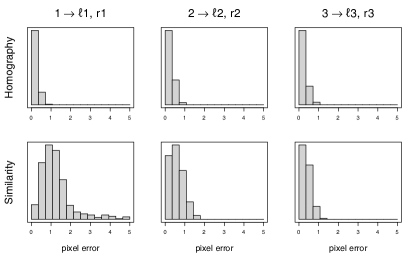
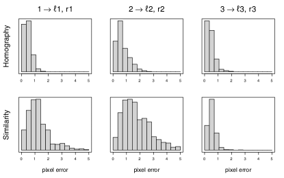
Figure 10: Calibration error (17), measured by projecting the fitted tof points $\mathitbf{Q}^{\pi}_{i}$ to the left and right rgb images ($1624\times 1224$) of the respective systems $i=1,2,3$. The tof/stereo alignment was computed via a 3-d homography (top), or a similarity transformation (bottom). It is clear that the former is superior, as described in section 4.3. The left and right $2\times 3$ blocks represent different capture-sessions, as described in the text.

4.4 Cross-calibration for 3-d reconstruction and rendering

The proposed cross-calibration methodology also allows a fully-textured 3-d model to be segmented and rendered. This is because the depth-data are automatically assigned to pixels in the rgb images. Figure 11 shows reconstruction instances with and without texture from a $360^{\circ}$ reconstruction, obtained from the cross-calibration of four tof+2rgb systems. Meshing was performed by the standard Poisson reconstruction method kazhdan-2006 , followed by simple triangle-based texture mapping.

More dense reconstruction can be achieved by exploiting the full resolution of stereo cameras, as described elsewhere gandhi-2012 . Figure 12 shows the difference between the raw reconstruction obtained from the cross-calibration of a tof+2rgb system, and that obtained after using the tof data in a subsequent stereo algorithm gandhi-2012 . A high-resolution depth map is produced, making full use of the high-resolution rgb cameras.

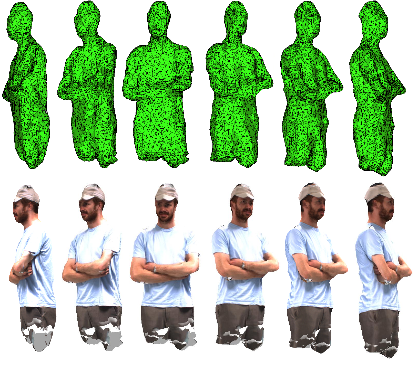
Figure 11: Examples of a segmented $360^{\circ}$ reconstruction, after Poisson meshing, with and without rgb texture.

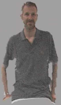
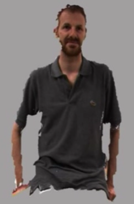
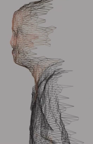
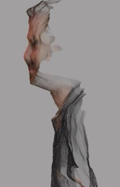
Figure 12: Cross-calibration for 3-d reconstruction. Left: The raw mesh, with textured edges, obtained directly from our tof+2rgb cross-calibration method. Right: The textured high-density point cloud, obtained after applying the tof-stereo fusion method of gandhi-2012 to the cross-calibration results.

5 Conclusion

It has been shown that 3-d projective transformations can be used to cross-calibrate a system of tof and stereo reconstructions. A practical method for computing these transformations, based on geometric principles, has been introduced. This calibration procedure has been extended to a nine-camera network of six rgb and three tof cameras, and evaluated in detail.

A clear distinction has been made between calibration error, which is due to imperfect camera and image models, versus total error, which incorporates tof-specific noise and biases. It has been shown that these errors can be separated geometrically, and used to characterize the performance of a tof/rgb camera network. The overall performance of the system has been visualized in segmented 360^∘ 3-d reconstructions. This type of reconstruction is challenging to compute, and shows that the system is more than adequate as a basis for scene-segmentation tasks.

The accuracy of the method presented here is somewhat limited by the relatively poor localization of points, even when spatially interpolated, in the tof images. The detection of standard chequerboard patterns, in tof images, has been discussed elsewhere hansard-2014 . The design of more convenient calibration patterns, for tof cameras, would be a worthwhile direction for future research. Meanwhile, in mitigation, the spatial resolution of tof cameras will continue to increase.

Future work should also consider the distribution of range-errors in 3-d, and how this can be used to design custom meshing and surface reconstruction algorithms for time-of-flight data. This, in conjunction with the rgb textures provided by the present method, would lead to a comprehensive approach to 3-d reconstruction, rendering and scene-understanding.

References

- (1) D. Hoiem, A. Efros, M. Hebert, Recovering surface layout from an image, International Journal of Computer Vision 75 (1) (2007) 151–172.
- (2) R. Tron, R. Vidal, A benchmark for the comparison of 3-d motion segmentation algorithms, in: Proc. CVPR’07, 2007, pp. 1–8.
- (3) S. Savarese, T. Tuytelaars, L. V. Gool, Special issue on 3D representation for object and scene recognition, Computer Vision and Image Understanding 113 (12) (2009) 1181–1182.
- (4) Z. Liu, M. Beetz, D. Cremers, J. Gall, W. Li, D. Pangercic, J. Sturm, Y.-W. Tai, Special issue on visual understanding and applications with RGB-D cameras, Journal of Visual Communication and Image Representation 25 (1).
- (5) A. Alahi, P. Vandergheynst, M. Bierlaire, M. Kunt, Cascade of descriptors to detect and track objects across any network of cameras, Computer Vision and Image Understanding 114 (6) (2010) 624–640.
- (6) Mesa Imaging, SR4000 Swiss Ranger manual, http://www.mesa-imaging.ch (2010).
- (7) M. Hansard, R. Horaud, M. Amat, G. Evangelidis, Automatic detection of calibration grids in time-of-flight images, Computer Vision and Image Understanding 121 (2014) 108–118.
- (8) A. Verri, V. Torre, Absolute depth estimate in stereopsis, J. Optical Society of America A 3 (3) (1986) 297–299.
- (9) M. Lindner, I. Schiller, A. Kolb, R. Koch, Time-of-flight sensor calibration for accurate range sensing, Computer Vision and Image Understanding 114 (12) (2010) 1318–1328.
- (10) A. Kolb, E. Barth, R. Koch, R. Larsen, Time-of-flight cameras in computer graphics, Computer Graphics Forum 29 (1) (2010) 141–159.
- (11) V. Gandhi, J. Cech, R. Horaud, High-resolution depth maps based on TOF-stereo fusion, in: Proc. ICRA, 2012, pp. 4742–4749.
- (12) R. Hartley, A. Zisserman, Multiple View Geometry in Computer Vision, Cambridge University Press, 2000.
- (13) R. Nair, K. Ruhl, S. Meister, H. Schäfer, C. S. Garbe, M. Eisemann, M. Magnor, D. Kondermann, A survey on time-of-flight stereo fusion, in: M. Grzegorzek, C. Theobalt, R. Koch, A. Kolb (Eds.), Time-of-Flight and Depth Imaging, Vol. 8200 of LNCS, Springer, 2013, Ch. A Survey on Time-of-Flight Stereo Fusion, pp. 105–127.
- (14) B. Huhle, S. Fleck, A. Schilling, Integrating 3D time-of-flight camera data and high resolution images for 3DTV applications, in: Proc. 3DTV, 2007, pp. 1–4.
- (15) B. Bartczak, R. Koch, Dense depth maps from low resolution time-of-flight depth and high resolution color views, in: Proc. Int. Symp. on Visual Computing (ISVC), 2009, pp. 228–239.
- (16) A. Bleiweiss, M. Werman, Fusing time-of-flight depth and color for real-time segmentation and tracking, in: Proc. DAGM Workshop on Dynamic 3D Imaging, 2009, pp. 58–69.
- (17) C. Beder, I. Schiller, R. Koch, Photoconsistent relative pose estimation between a PMD 2D3D-camera and multiple intensity cameras, in: Proc. Symp. of the German Association for Pattern Recognition (DAGM), 2008, pp. 264–273.
- (18) I. Schiller, C. Beder, R. Koch, Calibration of a PMD camera using a planar calibration object together with a multi-camera setup, in: Int. Arch. Soc. Photogrammetry, Remote Sensing and Spatial Information Sciences XXI, 2008, pp. 297–302.
- (19) R. Koch, I. Schiller, B. Bartczak, F. Kellner, K. Köser, MixIn3D: 3D mixed reality with ToF-camera, in: Proc. DAGM Workshop on dynamic 3D imaging, 2009, pp. 126–141.
- (20) J. Zhu, L. Wang, R. Yang, J. Davis, Z. Pan, Reliability fusion of time-of-flight depth and stereo geometry for high quality depth maps, IEEE Trans. on PAMI 33 (7) (2011) 1400–1414.
- (21) J. Zhu, L. Wang, R. G. Yang, J. Davis, Fusion of time-of-flight depth and stereo for high accuracy depth maps, in: Proc. CVPR, 2008, pp. 1–8.
- (22) Y. Wang, Y. Jia, A fusion framework of stereo vision and kinect for high-quality dense depth maps, in: ACCV 2012 Workshops, 2012, pp. 109–120.
- (23) J. Wu, Y. Zhou, H. Yu, Z. Zhang, Improved 3D depth image estimation algorithm for visual camera, in: Proc. International Congress on Image and Signal Processing, 2009, pp. 1–4.
- (24) J. Mure-Dubois, H. Hügli, Fusion of time-of-flight camera point clouds, in: ECCV Workshop on Multi-Camera and Multi-modal Sensor Fusion Algorithms and Applications, 2008.
- (25) M. Silva, R. Ferreira, J. Gaspar, Camera Calibration using a Color-Depth Camera: Points and Lines Based DLT including Radial Distortion, in: Proc. of IROS Workshop in Color-Depth Camera Fusion in Robotics, 2012.
- (26) C. Zhang, Z. Zhang, Calibration between depth and color sensors for commodity depth cameras, in: Proc. of the 2011 IEEE Int. Conf. on Multimedia and Expo, ICME ’11, 2011, pp. 1–6.
- (27) Z. Zhang, Flexible camera calibration by viewing a plane from unknown orientations, in: Proc. ICCV’99, 1999, pp. 666–673.
- (28) Y. Kim, D. Chan, C. Theobalt, S. Thrun, Design and calibration of a multi-view TOF sensor fusion system, in: Proc. CVPR Workshop on time-of-flight Camera based Computer Vision, 2008, pp. 1–7.
- (29) D. Herrera, J. Kannala, J. Heikila, Joint Depth and Color Camera Calibration with Distortion Correction, IEEE Trans. PAMI 34 (10) (2012) 2058–2064.
- (30) A. Teichman, S. Miller, S. Thrun, Unsupervised intrinsic calibration of depth sensors via slam, in: Proceedings of Robotics: Science and Systems, 2013.
-
(31)
I. V. Mikhelsona, P. G. Leea, A. V. Sahakiana, Y. Wua, A. K. Katsaggelosa,
Automatic, fast, online
calibration between depth and color cameras, Journal of Visual
Communication and Image RepresentationIn Press (available online).
URL http://dx.doi.org/10.1016/j.bbr.2011.03.031 - (32) Y. Cui, S. Schuon, S. Thrun, D. Stricker, C. Theobalt, Algorithms for 3d shape scanning with a depth camera, IEEE Trans. PAMI 35 (5) (2013) 1039–1050.
- (33) M. Hansard, R. Horaud, M. Amat, S. Lee, Projective Alignment of Range and Parallax Data, in: Proc. CVPR, 2011, pp. 3089–3096.
- (34) M. Hansard, S. Lee, O. Choi, R. Horaud, Time-of-Flight Cameras: Principles, Methods and Applications, Springer, 2013.
- (35) C. Beder, B. Bartczak, R. Koch, A comparison of PMD-cameras and stereo-vision for the task of surface reconstruction using patchlets, in: Proc. CVPR, 2007, pp. 1–8.
- (36) M. Hebert, E. Krotkov, 3D measurements from imaging laser radars: How good are they?, Image and Vision Computing 10 (3) (1992) 170–178.
- (37) C. Wang, H. Tanahasi, H. Hirayu, Y. Niwa, K. Yamamoto, Comparison of local plane fitting methods for range data, in: Proc. CVPR, 2001, pp. 663–669.
- (38) Y. Kanazawa, K. Kanatani, Reliability of Plane Fitting by Range Sensing, in: Proc. ICRA, 1995, pp. 2037–2042.
- (39) K. Pathak, N. Vaskevicius, A. Birk, Revisiting uncertainty analysis for optimum planes extracted from 3D range sensor point-clouds, in: Proc. ICRA, 2009, pp. 1631–1636.
- (40) G. Csurka, D. Demirdjian, R. Horaud, Finding the collineation between two projective reconstructions, Computer Vision and Image Understanding 75 (3) (1999) 260–268.
- (41) W. Förstner, Uncertainty and projective geometry, in: E. Bayro-Corrochano (Ed.), Handbook of Geometric Computing, Springer, 2005, pp. 493–534.
- (42) W. H. Press, S. A. Teukolsky, W. T. Vetterling, B. P. Flannery, Numerical Recipes in C, 2nd Edition, Cambridge University Press, 1992.
- (43) R. Hartley, P. Sturm, Triangulation, Computer Vision and Image Understanding 68 (2) (1997) 146–157.
- (44) K. Arun, T. S. Huang, S. D. Blostein, Least-squares fitting of two 3-D point sets, IEEE Trans. PAMI 9 (5) (1987) 698–700.
- (45) G. D. Evangelidis, E. Z. Psarakis, Parametric image alignment using enhanced correlation coefficient maximisation, IEEE Trans. PAMI 30 (10) (2010) 1858–1865.
- (46) S. Foix, G. Alenya, C. Torras, Lock-in Time-of-Flight (ToF) Cameras: A Survey, IEEE Sensors 11 (9) (2011) 1917–1926.
- (47) P. Schönemann, R. Carroll, Fitting one matrix to another under choice of a central dilation and a rigid motion, Psychometrika 35 (2) (1970) 245–255.
- (48) B. Horn, H. Hilden, S. Negahdaripour, Closed-form solution of absolute orientation using orthonormal matrices, J. Optical Society of America A 5 (7) (1988) 1127–1135.
- (49) M. M. Kazhdan, M. Bolitho, H. Hoppe, Poisson surface reconstruction, in: Symposium on Geometry Processing, 2006, pp. 61–70.