Quantitative constraints on starburst cycles in galaxies with stellar masses in the range $10^{8}-10^{10}M_{\odot}$

Abstract

We have used 4000 Å break and H$\delta_{A}$ indices in combination with SFR/$M_{*}$ derived from emission line flux measurements, to constrain the recent star formation histories of galaxies with stellar masses in the range $10^{8}-10^{10}M_{\odot}$. The fraction of the total SFR density in galaxies with ongoing bursts is a strong function of stellar mass, declining from 0.85 at a stellar mass of $10^{8}M_{\odot}$ to 0.25 for galaxies with $M_{*}\sim 10^{10}M_{\odot}$. Low mass galaxies are not all young. The distribution of half mass formation times for galaxies with stellar masses less than $10^{9}M_{\odot}$ is broad, spanning the range 1-10 Gyr. The peak-to-trough variation in star formation rate among the bursting population ranges lies in the range 10-25. In low mass galaxies, the average duration of the burst bursts is comparable to the dynamical time of the galaxy. Galaxy structure is correlated with estimated burst mass fraction, but in different ways in low and high mass galaxies. High mass galaxies with large burst mass fractions are more centrally concentrated, indicating that bulge formation is at work. In low mass galaxies, stellar surface densities $\mu_{*}$ decrease as a function of $F_{burst}$. These results are in good agreement with the observational predictions of Teyssier et al (2013) and lend further credence to the idea that the cuspy halo problem can be solved by energy input from multiple starbursts over the lifetime of the galaxy. We note that there is no compelling evidence for IMF variations in the population of star-forming galaxies in the local Universe.

1 Introduction

Cosmological simulations of the evolution of cold dark matter (CDM) show that the dark matter in collapsed, virialized systems forms cuspy distributions with inner profiles that are too steep compared with observations (e.g. Flores & Primack 1994; Moore 1994; Navarro, Frenk & White 1996). This is commonly referred to as the cuspy halo problem. One solution to this problem proposed early on, is that that impulsive mass loss from the galaxy can lead to irreversible expansion of the orbits of stars and dark matter near the center of the halo (Navarro, Eke & Frenk 1996; Read & Gilmore 2005; Pontzen & Governato 2012). These conclusions were based on simple analytic arguments and it was not clear whether this mechanism could in fact produce central density profiles in close agreement with observations. Recently, there have been a series of gas-dynamical simulations of dwarf galaxies demonstrating that repeated gas outflows during bursts of star formation can indeed transfer enough energy to the dark matter component to flatten “cuspy” central dark matter profiles (Mashchenko, Wadsley & Couchman 2008; Governato et al 2010; Governato et al 2012; Zolotov et al 2012; Trujillo-Gomez et al 2013; Teyssier et al 2013; Shen et al 2013).

It is still unclear whether the energy requirements for flattening cuspy profiles are in line with the actual stellar populations and star formation histories of real low mass galaxies (Gnedin & Zhao 2002; Garrison-Kimmel et al 2013). In a recent paper, Teyssier et al (2013) highlighted two key observational predictions of all simulations that find cusp-core transformations: i) low mass galaxies have a bursty star formation history with a peak-to-trough ratio of 5 to 10, ii) the bursts occur on the dynamical timescale of the galaxy. In addition, the simulations show that the feedback associated with the bursts alter the final stellar structure of the galaxies. In simulations without feedback, a prominent bulge with large Sersic index and a weak exponential disk was formed. In contrast, in the simulation with feedback, a smaller exponential disk with no bulge in the center and a clear signature of a core within the central 500 pc was produced.

Observationally, it is well established that there exist classes of low mass galaxy, for example blue compact dwarf galaxies with strong emission lines (BCD galaxies), which are clearly undergoing strong starbursts at the present day (e.g. Searle & Sargent 1972; Meurer et al 1995). In very nearby galaxies where individual stars can be resolved in high quality images, star formation histories for individual systems can be derived over longer timescales. Some nearby dwarf spheroidals have clearly experienced bursty star formation histories in their past (e.g. Dolphin 2012; De Boer et al 2012). On the other hand, the star formation histories of dwarf irregular galaxies have been found to be relatively quiescent (e.g. Van Zee 2001).

Recent work on low mass galaxies at high redshifts by Van der Wel et al (2011) has indicated that the space densities of extreme emission line dwarf galaxies with stellar masses $\sim 10^{8}M_{\odot}$ are much higher at earlier cosmic times. At $z>1$, these authors claim that the population of extreme emission line galaxies detected in the CANDELS survey is high enough to produce a significant fraction of the total stellar mass contained in the present-day population of such galaxies, if star formation continued in the same mode for around 4 Gyr. These authors propose that most of the stars in present-day dwarf galaxies must have formed in strong bursts at $z>1$. This conclusion is, however, at odds with the observation that the stellar populations of present-day low mass galaxies are, on average, quite young (Kauffmann et al 2003b). Heavens et al (2004) analyzed the star formation histories of stacked samples of galaxies in bins of stellar mass from the Sloan Digital Sky survey. They showed that the average star formation history of galaxies with stellar masses less than $10^{10}M_{\odot}$ could be well represented by flat star formation rate over the past 3-7 Gyr, with a decline at earlier epochs.

In order to estimate the duty cycle of the starburst phenomenon as well as the amplitude range in star formation during a burst, it is necessary to analyze a complete sample of galaxies that are intrinsically similar. Kauffmann et al (2003b) used constraints from 4000 Å break and H$\delta_{A}$ stellar absorption line indices to show that the fraction of present-day galaxies that have experienced bursts in the past 1-2 Gyr, is a factor of 5 higher for galaxies with stellar masses $\sim 10^{8}M_{\odot}$ than for galaxies with $M_{*}\sim 10^{10}M_{\odot}$. A similar conclusion was recently reached by Bauer et al (2013), who analyzed the distribution of specific star formation rates as a function of stellar mass for galaxies with $0.05<z<0.32$ from the Galaxy and Mass Assembly (GAMA) survey and found a significant tail of galaxies with high SFR/M_∗ and low stellar masses that could only be explained by a stochastic burst with late onset.

In this paper, we use the 4000 Å break and H$\delta_{A}$ indices in combination with SFR/$M_{*}$ derived from emission line flux measurements, to constrain the recent star formation histories of low mass galaxies. We show that this combination of quantities allows us to clearly separate galaxies that are currently undergoing a burst of star formation from galaxies that have formed their stars continuously and galaxies that have experienced a burst in the past. We use the subsample of galaxies experiencing an ongoing burst to constrain burst mass fractions and duty cycles, as well as the amplitude variation in SFR/M_∗ during the burst. We investigate how these parameters change as a function of galaxy mass. Finally, we investigate how the stellar structure of the galaxy correlates with burst mass fraction. The paper is organized as follows: in section 2, we describe or sample and the methodology we use to analyze star formation histories. In section 3, we present our results, and in section 4, we summarize and conclude. A Hubble constant $H_{0}=70$ km s^-1 is adopted throughout.

2 Data Analysis Methodology

2.1 The Sample

The parent galaxy sample used in this study is a magnitude-limited sample constructed from the final data release (DR7; Abazajian et al. 2009) of the SDSS (York et al. 2000) and is the same as that used in Li et al. (2012). This sample contains 482,755 galaxies located in the main contiguous area of the survey in the northern Galactic cap, with $r<17.6$, $24<M_{0.1r}<16$ and spectroscopically measured redshifts in the range $0.001<z<0.5$. Here $r$ is the $r$-band Petrosian apparent magnitude, corrected for Galactic extinction, and $M_{0.1r}$ is the $r$-band Petrosian absolute magnitude, corrected for evolution and K-corrected to its value at z=0.1.

Stellar masses, D_n(4000) and H$\delta_{A}$ line index measurements from the SDSS fiber spectra, as well as the estimated error on these quantities, are taken from the DR7 MPA/JHU value added catalogue (http://www.mpa-garching.mpg.de/SDSS/DR7/).

Star formation rates estimated within a 3 arcsecond fiber aperture are also available from these catalogues. The reader is referred to Brinchmann et al. (2004) for a detailed description of how SFRs are derived. Briefly, star formation rates are estimated by fitting a grid of photo-ionization models to the observed [OIII], H$\beta$, H$\alpha$ and [NII] line strengths for galaxies where the [OIII]/H$\beta$ and [NII]/H$\alpha$ line ratios have values that place them within the region of the Baldwin, Phillips & Terlevich (1981, BPT) diagram occupied by galaxies in which the primary source of ionizing photons is from HII regions rather than an active galactic nucleus (AGN). Standard Bayesian estimation methodology is used to derive the probability distribution function (PDF) of the star formation rate. We adopt the median of the integrated PDF as our actual estimate and one half the difference between the 84th and 16th percentile points as our estimate of the 1$\sigma$ error. We note that if the H$\beta$ line is not detected, the [NII]/H$\alpha$ ratio can still be used to separate out AGN; in this case, the SFR estimates have much larger errors, because dust extinction is not well constrained.

The MPA/JHU catalogue does contain SFR estimates for AGN and galaxies where the H$\alpha$ and/or [NII] lines are not detected. These estimates are derived using an empirical calibration between D_n(4000) and SFR/$M_{*}$ (see Brinchmann et al 2004 for details). For such objects, the SFR estimates carry no direct information about HII region line luminosities and thus cannot be used to find galaxies that are experiencing ongoing bursts. For this reason, we restrict the discussion in this paper to galaxies with $M_{*}<10^{10}M_{\odot}$, where the fraction of AGN drops to values close to zero (Kauffmann et al 2003c). In this case, essentially all galaxies with indirect SFR estimates are those with no detection of H$\alpha$/[NII]. These galaxies have old stellar populations, and as will be discussed in the next section, they are classified as having had quiescent star formation histories.

2.2 Methodology for constraining star formation histories

We create three different model libraries by using the population synthesis code of Bruzual & Charlot (2003) as follows:

1. Continuous Models. – a library of model galaxies with continuous star formation histories. These model galaxies have a continuous SFR, declining exponentially according to SFR(t) $\propto e^{-\gamma t}$, with $\gamma$ uniformly distributed between 0 (i.e. constant star formation rate) and 0.5 Gyr^-1. Stars begin to form at a look-back times between 11.375 Gyr and 4.2 Gyr in the past. We output the spectral energy distribution parameters at the present day.

2. Models with ongoing bursts. For each model galaxy in the continuous library described above, we add a burst which starts 100 million years before the present time. The burst has constant amplitude as a function of time and the amplitudes are allowed to vary so that the mass fraction of stars formed in the burst ranges from 0.00001 to close to 1. We output the spectral energy distribution parameters at time intervals $\Delta t$ of 10 million years while the burst is in progress.

3. Models with past bursts. We follow the same algorithm used to create the models with ongoing bursts, except that the starting time for the burst ranges from 2 Gyr before the present to 0.2 Gyr before the present. All bursts run for a total duration of 100 million years. We output spectral energy distribution parameters at the present day.

We generate all model libraries at metallicities of 0.5 solar and 0.25 solar, appropriate for galaxies with stellar masses in the range $10^{8}$ to $10^{10}M_{\odot}$ (Tremonti et al 2004). A fixed Chabrier (2003) initial mass function (IMF) is adopted for all the models.

The first three panels of Figure 1 show the distribution of model galaxies in the plane of specific star formation rate (SFR/M_∗) versus D_n(4000), H$\delta_{A}$ versus D_n(4000), and SFR/M_∗ versus H$\delta_{A}$. Model galaxies in the continuous libraries are coloured in green, those in the ongoing burst library and coloured in blue and those in the past burst library are coloured in red. As can be seen, the models with ongoing and past bursts are well separated, particularly in the SFR/M_∗ versus D_n(4000) and the SFR/M_∗ versus H$\delta_{A}$ planes. Continuous models occupy a narrow locus between the region of the diagrams spanned by the two classes of burst models. The locus is particularly narrow for galaxies with young stellar populations (D_n(4000) $<1.5$, H$\delta_{A}>3$). The continuous models fan out at older ages, where metallicity affects the 4000 Å break strength (Kauffmann et al 2003a) and the choice of formation time limits the age of the oldest stars in the model galaxies.

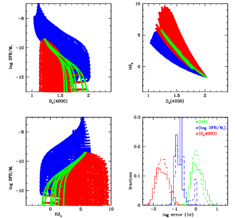
Figure 1: The first three panels show the distribution of model galaxies in the plane of specific star formation rate (SFR/M_∗) versus D_n(4000), H$\delta_{A}$ versus D_n(4000), and SFR/M_∗ versus H$\delta_{A}$. Model galaxies in the continuous libraries are coloured in green, those in the ongoing burst library and coloured in blue and those in the past burst library are coloured in red. In the bottom right panel, we plot histograms of the 1$\sigma$ errors on D_n(4000), H$\delta_{A}$ and SFR/M_∗.

Our ability to use the model library to constrain star formation histories will depend on the precision to which the quantities D_n(4000), H$\delta_{A}$ and SFR/$M_{*}$ can be measured. In the bottom right panel of Figure 1, we plot histograms of the 1$\sigma$ errors on D_n(4000), H$\delta_{A}$ and SFR/M_∗. Solid histograms show results for low mass galaxies ($\log M_{*}\sim 8.5$), while dashed histograms show results for high mass galaxies ($\log M_{*}\sim 10$). The error distribution depends very little on mass. The typical error on D_n(4000) is a few percent, while the errors on H$\delta_{A}$ are around 10%. log SFR/M_∗ is measured with a formal error of 0.1-0.2 dex. We note that the SFR/M_∗ error estimate does not include any estimate of the systematic errors in the photo-ionization models used to estimate SFR. Nevertheless, it is clear from Figure 1 that we should be able to separate galaxies with ongoing starbursts from the rest of the population with reasonably high confidence.

2.3 Classification and Parameterization of Star Formation History

We now describe the procedure used to group galaxies into classes according to whether they most likely have had continuous star formation histories, are currently experiencing a burst, or have experienced a burst in the past 2 Gyr. We note that these classifications pertain to the central regions of the galaxies, since the fiber spectrum typically samples 20-30 % of the total light from the galaxy (Kauffmann et al 2003a). We first search the continuous star formation library for the model that minimizes $\chi^{2}$. If the minimum $\chi^{2}$ per degree of freedom ($\chi^{2}_{min}/N_{d}$, with $N_{d}=3$ in our case) is less than 2.37, this means that there is a 50% or greater probability that that the continuous SFH hypothesis is correct, and we place the galaxy into the continuous class.

If $\chi^{2}_{min}/N_{d}$ is greater than 2.37, we then search both the ongoing and past burst libraries for a new minimum $\chi^{2}$ model. We check whether the new $\chi^{2}_{min}/N_{d}$ is smaller than that obtained for the continuous library, and smaller than 2.37. If so, we consider our classification into ongoing burst/past burst as “secure”. We note that the burst libraries contain models with burst fractions very close to zero, which are essentially identical to the models in the continuous library, so the new minimum $\chi^{2}$ is guaranteed to be equal to or smaller than the old one. If the new $\chi^{2}_{min}/N_{d}$ lies in the range 2.37-6.25, the probability that the model is consistent with the data is still between 10-50%, so these classifications should be regarded as ”tentative”.

In Figure 2, we plot galaxies in the stellar mass range $10^{9.75}-10^{10}M_{\odot}$ in the plane of log SFR/$M_{*}$ versus D_n(4000) and log SFR/M_∗ versus H$\delta_{A}$. We colour-code the points according to their classification: black refers to continuous, blue to ongoing burst and red to past burst. This particular mass range is chosen mainly for illustrative purposes. As can be seen, most of the leverage in the classification comes from the combination of SFR/$M_{*}$ and D_n(4000) where the three classes separate most clearly. This is not surprising, because we have seen that these two quantities have smaller errors than H$\delta_{A}$. It should also be noted that the class of galaxies that are experiencing ongoing bursts is clearly separated from the the other two classes in both planes. They appear as a very distinct cloud of points extending to high values of SFR/$M_{*}$ and low/high values of D_n(4000)/H$\delta_{A}$. The models in Figure 1 include many objects with underlying old stellar populations that are currently undergoing a burst. These appear at high values of SFR/$M_{*}$ and high/low values of D_n(4000)/H$\delta_{A}$. However, galaxies of this type do not appear to be present in the real data.

We comment briefly on the very narrow tail of black points in the left panel of Figure 2. This is the minority population of quiescent galaxies and/or AGN for which SFR is not estimated using emission lines, but using D_n(4000). In the lower mass ranges, this tail disappears altogether.

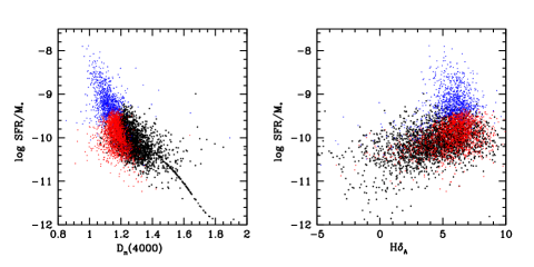
Figure 2: Galaxies in the stellar mass range $10^{9.75}-10^{10}M_{\odot}$ in the plane of log SFR/$M_{*}$ versus D_n(4000) and log SFR/M_∗ versus H$\delta_{A}$ We colour-code the points according to their classification: black refers to continuous, blue to ongoing burst and red to past burst.

We note that for each model galaxy, we store a variety of parameters relating to its star formation history. We can then use the library to compute the most probable value of each parameter from the median of the likelihood distribution, and an error on each parameter from the range enclosing 68 percent of the total probability density (see the Appendix in Kauffmann et al 2003a). The two parameters that will be explored in this paper include the fraction of the total stellar mass of the galaxy formed in the starburst and a formation time, defined to be the lookback time when half the stars in the galaxy were formed.

2.4 Evidence for IMF variations?

It is interesting to investigate the population of galaxies with minimum reduced $\chi^{2}$ values greater than 6.25, in order to see whether there is any evidence that our underlying stellar population models do not represent the data adequately. One possible inadequacy is the assumption of a fixed Chabrier IMF. Changing the fraction of high mass stars would alter the locus of the models in the plane of inferred SFR/$M_{*}$ versus D_n(4000)/H$\delta_{A}$. Systematic variations in the top-end of the IMF have been claimed by Hoversten & Glazebrook (2008) and Gunawardhana et al (2011) based on a changing relation between H$\alpha$ equivalent width and broad-band colour, and by Meurer et al (2009) based on a changing relation between H$\alpha$ and the UV luminosities in galaxies. We note that previous work did not attempt to account for the effect of bursts on a galaxy-by-galaxy basis. In addition, the test using H$\alpha$-based SFR and two narrow-band stellar absorption line indices should be less sensitive to systematic effects in the procedures used to correct for dust extinction.

We find the fraction of galaxies with $\chi^{2}_{min}/N_{d}$ values greater than 6.25 to be $\sim$ 5%. These outliers are primarily galaxies with low 4000 Å break strengths and strong emission lines. The greatest discrepancy between models and data arises for the H$\delta_{A}$ index. We note that in strongly star-bursting galaxies, the H$\delta_{A}$ absorption feature is filled in by nebular emission. Although the MPA/JHU spectral fitting pipeline attempts to subtract the emission, recovery of the H$\delta$ absorption features can be expected to become increasingly inaccurate for strongly star-bursting galaxies where stellar features are weak and nebular emission dominates. We therefore perform a restricted fit to the combination of SFR/M_∗ and D_n(4000). The percentage of galaxies with $\chi^{2}_{min}/N_{d}$ values greater than 4.61 (corresponding to a probability of 0.1 for 2 degrees of freedom) drops by another factor of two to values less than $\sim$2-3% in all the stellar mass bins. The remaining outliers mainly have D_n(4000) values that are less than 1, a value that cannot be matched by the youngest stellar template in the Bruzual & Charlot (2003) models. We have checked the dependence of D_n(4000) on IMF slope and on whether nebular continuum emission is included using the STARBURST 99 models (Leitherer et al 1999). Our tests show that D_n(4000)$<1$ cannot be reached by tuning these parameters. We think it is most likely that the remaining outliers are affected by errors in the spectro-photometric flux calibration. In summary, we find do not find a population of galaxies where there is conclusive evidence for a top-heavy IMF, though we feel that it would be premature to rule out IMF variations based on this data.

3 Results

3.1 Contribution of bursts to the SFR density

The black curve in Figure 3 shows the fraction of the total integrated stellar mass in galaxies that resides in galaxies that are well-fit by continuous models. The mass fraction increases from 0.3 for galaxies with $M_{*}=10^{8}M_{\odot}$ to 0.9 for galaxies with $M_{*}=10^{10.25}M_{\odot}$. The blue curve shows the fraction of the total integrated star formation rate density in galaxies with continuous star formation histories. This rises from 0.05 at the low mass end to 0.7 at the high mass end. The cyan curve shows the fraction of the total integrated star formation rate density in galaxies currently undergoing a starburst. According to Heckman et al (1997a), at least 25% of the high-mass star-formation in the local universe occurs in starbursts, a number that agrees well with our results at $M_{*}=10^{10.25}M_{\odot}$. We note that the difference between unity and the sum of the blue and cyan curves corresponds to the fraction of the integrated SFR density in galaxies that are best fit by models with past bursts. This generally lies in the range 0.1-0.2.

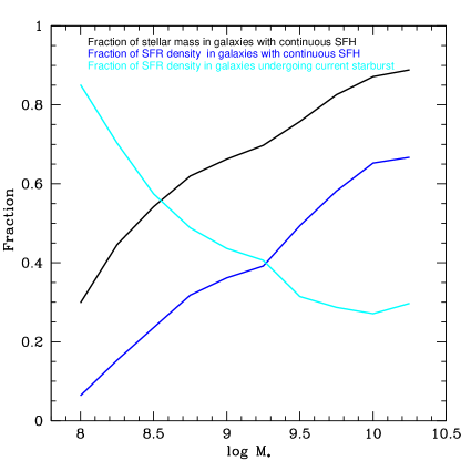
Figure 3: The black curve shows the fraction of the total integrated stellar mass in galaxies that resides in galaxies that are well-fit by continuous models. The blue curve shows the fraction of the total integrated star formation rate density in galaxies with continuous star formation histories. The cyan curve shows the fraction of the total integrated star formation rate density in galaxies currently undergoing a starburst.

3.2 Burst mass fractions

In Figure 4, we plot distributions of burst mass fractions for the population of galaxies currently undergoing starbursts. The burst mass fraction is defined as the stellar mass formed in the burst divided by the total stellar mass of the galaxy. Results are shown in 9 different mass ranges from 8.0 to 10.25 in log $M_{*}$. As can be seen, there is a significant tail of low mass galaxies with burst mass fractions larger than 0.3 for the lowest mass bins. The tail of galaxies with large burst mass fractions disappears progressively towards higher stellar masses. For galaxies with stellar masses $\sim 10^{10}M_{\odot}$, the burst mass fraction is typically around 0.05-0.1. The red dotted histograms in each panel shows the distribution of the relative errors on $F_{burst}$, i.e. the error scaled by dividing by the actual estimate. As can be seen, burst mass fractions can be recovered with a typical accuracies of between 25 and 60% (i.e. significantly better than a factor of two). The error distribution does not change significantly as a function of stellar mass, indicating that the trend in the tail of strong starbursts is not an artifact of increasing errors at low stellar masses.

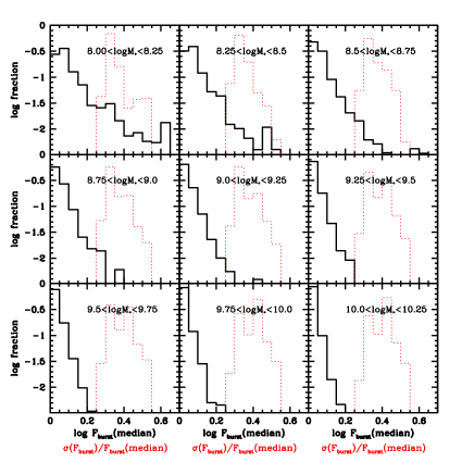
Figure 4: Histograms (in black) of the distribution of the logarithm of the burst mass fraction. Results are shown in 9 different mass ranges from 8.0 to 10.25 in log $M_{*}$. The red dotted histograms in each panel show the distribution of the relative error on $F_{burst}$.

3.3 Half mass formation times

In Figure 5, we plot distributions of half-mass formation times for all galaxies in the same 9 stellar mass ranges. Interestingly, in the lowest mass bin where the fraction of galaxies experiencing ongoing starbursts is highest, the distribution of half-mass formation times is very broad, ranging from 10 Gyr to less than 1 Gyr. In the intermediate mass bins, the distribution is narrower, ranging from 7 to 3 Gyr. In the highest mass bins, a tail of galaxies with large ($\sim$ 10 Gyr) formation times again appears. These results should be compared to the distribution of 4000 Å break strength shown in Figure 2 of Kauffmann et al (2003b). This plot shows a monotonic increase as a function of stellar mass, with a secondary tail of large D_n(4000) galaxies appearing at the same stellar mass where we see the large half-mass formation time tail appear for the second time.

These results may appear puzzling at first sight, but we remind the reader that a one-to-one mapping between 4000 Å break strength and half mass formation time only exists if the underlying star formation history is continuous. If star formation is bursty, D_n(4000) alone cannot be used to infer formation time. The dotted red histograms in each panel show the distribution of 1$\sigma$ errors on the formation time, which are in the range 0.5-2.5 Gyr. Once again the error distributions do not vary significantly as a function of stellar mass, indicating that the greater spread at low stellar masses is a real effect.

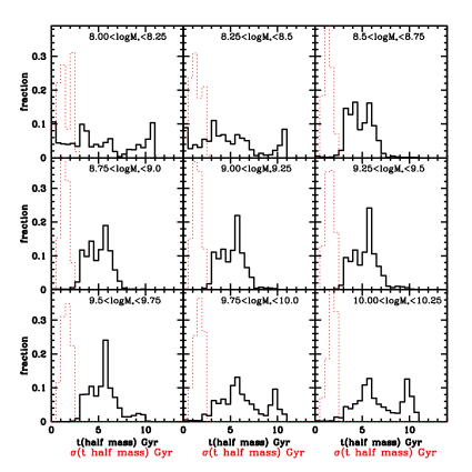
Figure 5: Histograms (in black) of the distribution of the half mass formation time. Results are shown in 9 different mass ranges from 8.0 to 10.25 in log $M_{*}$. The red dotted histograms in each panel show the distribution of the error on $t_{halfmass}$.

3.4 Correlation between burst mass fraction and galaxy structure and metallicity

We now investigate whether there is any direct observational evidence that bursts are correlated with changes in the metallicities and structural properties of galaxies. The structural properties include the stellar surface mass density $\mu_{*}$, where $\mu_{*}=0.5M_{*}/\pi R_{50}^{2}$ (R₅₀ is the half-light radius of the galaxy), and the concentration index $R_{90}/R_{50}$, where $R_{90}$ is the radius enclosing 90% of the light of the galaxy. The concentration index is often used as a rough proxy for galaxy bulge-to-disk ratio (Shimasaku et al 2001). The metallicity is the gas-phase metallicity derived from emission line ratios using the methodology described in Tremonti et al (2004).

The solid curves in Figure 6 show how the median values of $\mu_{*}$, R90/R50 and gas-phase metallicity vary as a function of $F_{burst}$ for galaxies with ongoing starbursts. Dashed curves indicate the 25th and 75th percentiles of the distribution of these quantities. Results are shown in three different mass ranges: $8<\log M_{*}<9$, $9<\log M_{*}<10$ and $10<\log M_{*}<10.5$. In the lowest mass bin, median stellar surface density decreases by 0.2-0.3 dex in log $\mu_{*}$ for the highest burst mass fractions. No significant trend is seen for concentration index. The gas-phase metallicity also drops by $\sim 0.2$ dex. In the two higher mass bins, the correlation between stellar mass density and burst mass fraction vanishes. Instead, there is a clear trend for concentration index to increase as a function of F_burst. The most natural interpretation of these results is that in high mass galaxies, starbursts result in the formation of a centrally-concentrated bulge component. In low mass galaxies, starbursts no longer build bulges. The feedback associated with the burst becomes strong enough to alter the stellar structure of the galaxy and reduce stellar densities as seen in the hydrodynamical simulations of dwarf galaxies discussed in Section 1.

Figure 6: Correlation between $\mu_{*}$, R90/R50 and gas-phase metallicity as a function of $F_{burst}$. Solid curves show the medians, while dashed curves indicate the 25th and 75th percentiles of the distribution of each of these quantities.

3.5 Environment

We note that a reduction in the gas-phase metallicities of interacting starburst galaxies in pairs compared to “normal” galaxies of the same stellar mass has been found in previous work by Kewley, Geller & Barton (2006). In Figure 7, we show an image gallery of galaxies with stellar masses less than $10^{9}M_{\odot}$ with burst mass fractions larger than 0.4. As can be seen, the majority are strongly asymmetric, but they are not always clearly interacting with another nearby galaxy. This is in agreement with work by Li et al. (2008), who found that a close neighbour is a sufficient, but not necessary condition for galaxies to be strongly star-forming. We have also investigated the environments of the star-bursting galaxies on larger scales by counting the number of spectroscopic neighbours within a projected radius of 1 Mpc and a velocity difference of less than 500 km/s. We find no significant differences with respect to galaxies with continuous star formation histories.

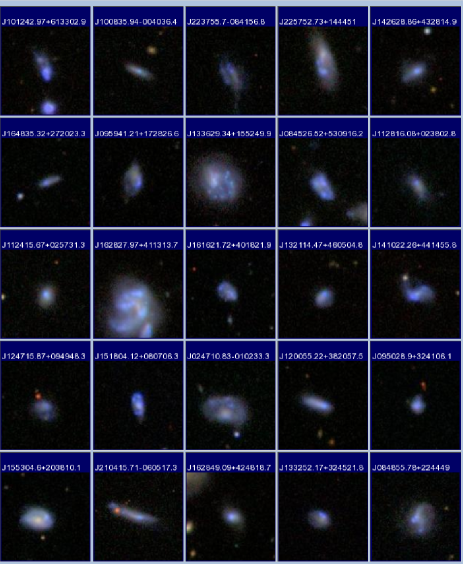
Figure 7: SDSS postage stamp images of some of the galaxies with burst mass fractions greater than 0.4 in the stellar mass range $10^{8.5}-10^{9}M_{\odot}$.

3.6 Burst amplitudes and durations

If we make the assumption that starburst galaxies with similar stellar masses represent a single class of object viewed a different times during the starburst cycle, the distribution function of SFR/$M_{*}$ provides the most direct constraint on the SFR amplitude variations during the burst. In Figure 8, we plot the cumulative distribution of galaxies with ongoing starbursts with SFR/$M_{*}$ values less than a given value. Cyan, blue, green, black, yellow, red and magenta curves represent galaxies in bins of increasing stellar mass from $10^{8}$ to $10^{10.25}M_{\odot}$. Dotted lines mark the 10th and 90th percentile points, which we adopt as our definition of peak-to-trough variation in amplitude. As can be seen the peak-to-trough variations range from a factor 25 for the lowest mass galaxies with $10^{8}-10^{9}M_{\odot}$ to a factor of 10 for galaxies with $\sim 10^{10}M_{\odot}$.

We can now combine these results from those presented in Figure 4 to estimate the average duration of the bursts in low mass galaxies. The median burst mass fraction in a galaxy with $10^{8}M_{\odot}$ is 0.05, which corresponds to a burst mass of $5\times 10^{6}M_{\odot}$. From Figure 8, the median specific star formation rate during the burst is log SFR/$M_{*}$ = -9.6, which corresponds to a star formation rate of 0.02511 $M_{\odot}$ yr^-1. This leads to an estimate of the typical period of the burst of $2\times 10^{8}$ yr. A $10^{8}M_{\odot}$ galaxy has a characteristic effective radius of 1.1 kpc (Kauffmann et al 2003b) and a rotation velocity of 80 km s^-1 (McGaugh et al 2000), which yields a dynamical time of $1.3\times 10^{8}$ yr. We conclude that the typical burst duration is very similar to the dynamical timescale of the galaxy. This, together with our estimates of peak-to-trough variation in SFR, are in good agreement with the requirements put forward by Teyssier et al (2013).

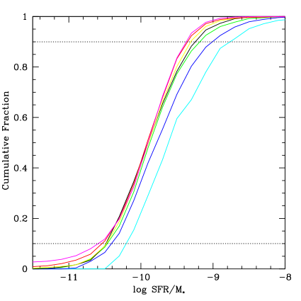
Figure 8: The cumulative distribution of galaxies with ongoing starbursts with SFR/$M_{*}$ values less than a given value. Cyan, blue, green, black, yellow, red and magenta curves represent galaxies in bins of increasing stellar mass from $10^{8}$ to $10^{10}M_{\odot}$. (Cyan: $10^{8}-10^{8.5}M_{\odot}$, Blue: $10^{8.5}-10^{8.75}M_{\odot}$, Green: $10^{8.75}-10^{9}M_{\odot}$, Yellow: $10^{9}-10^{9.25}M_{\odot}$, Red: $10^{9.25}-10^{9.5}M_{\odot}$, Magenta: $10^{9.5}-10^{9.75}M_{\odot}$.) Dotted lines mark the 10th and 90th percentile points, which we adopt as our definition of ”peak-to-trough” variation in amplitude.

4 Summary

We have used the the 4000 Å break and H$\delta_{A}$ indices in combination with SFR/$M_{*}$ derived from emission line flux measurements, to constrain the recent star formation histories of galaxies in the stellar mass range $10^{8}-10^{10}M_{\odot}$. Our main results can be summarized as follows.

• The fraction of the total SFR density in galaxies with ongoing bursts declines with increasing stellar mass, from 0.85 at a stellar mass of $10^{8}M_{\odot}$ to 0.25 at a stellar mass of $10^{10}M_{\odot}$. The duty cycle of bursts declines from 0.7 for $10^{8}M_{\odot}$ galaxies to 0.1 for $10^{10}M_{\odot}$ galaxies.

• The median burst mass fraction in galaxies of all stellar masses is small, 5% or less. There is, however, a tail of low mass galaxies that are undergoing bursts that have formed as much as 50-60% of their present-day mass. The number of galaxies in this high mass fraction tail decreases as a function of stellar mass.

• Low mass galaxies are not all young. The distribution of half mass formation times for galaxies with stellar masses less than $10^{9}M_{\odot}$ is broad, spanning the range from 1 to 10 Gyr. This is quite different to what is obtained when colours or 4000 Å break strengths are used to estimate stellar population age, assuming continuous star formation histories.

• The peak-to-trough variation in star formation rate among the bursting population ranges from a factor of 25 in the lowest mass galaxies in our sample to a factor of 10 for galaxies with $M_{*}=10^{10}M_{\odot}$. The average duration of bursts in low mass galaxies is comparable to their average dynamical time.

• Burst mass fraction is correlated with galaxy structure in quite different ways in low and high mass galaxies. High mass galaxies experiencing strong bursts are more centrally concentrated, indicating that bulge formation is likely at work. This is not seen in low mass galaxies. In low mass galaxies, we find that the stellar surface densities decrease as a function of $F_{burst}$.

• Gas phase metallicities decrease as a function of $F_{burst}$ in galaxies of all stellar masses.

These results are in rather good agreement with the observational predictions of Teyssier et al (2013) and lend further credence to the idea that the cuspy halo problem can be solved by energy input from multiple starbursts triggered by gas cooling and supernova feedback cycles over the history of a low mass galaxy. We note that the analysis in this paper is confined to the stellar populations enclosed within the 3 arsecond diameter fiber aperture, which samples the central $\sim$ 20-30 % of the total light from the galaxy. In future, it will be interesting to obtain resolved kinematic data for complete samples of low mass galaxies to understand the influence of bursts on galaxy and dark matter halo structure in more detail.

References

- Abazajian et al. (2009) Abazajian K. N., et al., 2009, ApJS, 182, 543
- Baldwin, Phillips, & Terlevich (1981) Baldwin J. A., Phillips M. M., Terlevich R., 1981, PASP, 93, 5
- Bauer et al. (2013) Bauer A. E., et al., 2013, MNRAS, 434, 209
- Brinchmann et al. (2004) Brinchmann J., Charlot S., White S. D. M., Tremonti C., Kauffmann G., Heckman T., Brinkmann J., 2004, MNRAS, 351, 1151
- Bruzual & Charlot (2003) Bruzual G., Charlot S., 2003, MNRAS, 344, 1000
- Chabrier (2003) Chabrier G., 2003, PASP, 115, 763
- de Boer et al. (2012) de Boer T. J. L., et al., 2012, A&A, 539, A103
- Dolphin (2012) Dolphin A. E., 2012, ApJ, 751, 60
- Flores & Primack (1994) Flores R. A., Primack J. R., 1994, ApJ, 427, L1
- Garrison-Kimmel et al. (2013) Garrison-Kimmel S., Rocha M., Boylan-Kolchin M., Bullock J. S., Lally J., 2013, MNRAS, 433, 3539
- Gnedin & Zhao (2002) Gnedin O. Y., Zhao H., 2002, MNRAS, 333, 299
- Governato et al. (2010) Governato F., et al., 2010, Natur, 463, 203
- Gunawardhana et al. (2011) Gunawardhana M. L. P., et al., 2011, MNRAS, 415, 1647
- Heavens et al. (2004) Heavens A., Panter B., Jimenez R., Dunlop J., 2004, Natur, 428, 625
- Heckman (1997) Heckman T. M., 1997, AIPC, 393, 271
- Hoversten & Glazebrook (2008) Hoversten E. A., Glazebrook K., 2008, ApJ, 675, 163
- Kauffmann et al. (2003) Kauffmann G., et al., 2003a, MNRAS, 341, 33
- Kauffmann et al. (2003) Kauffmann G., et al., 2003b, MNRAS, 341, 54
- Kauffmann et al. (2003) Kauffmann G., et al., 2003c, MNRAS, 346, 1055
- Kewley, Geller, & Barton (2006) Kewley L. J., Geller M. J., Barton E. J., 2006, AJ, 131, 2004
- Leitherer et al. (1999) Leitherer C., et al., 1999, ApJS, 123, 3
- Li et al. (2008) Li C., Kauffmann G., Heckman T. M., Jing Y. P., White S. D. M., 2008, MNRAS, 385, 1903
- Li et al. (2012) Li C., et al., 2012, MNRAS, 419, 1557
- Mashchenko, Wadsley, & Couchman (2008) Mashchenko S., Wadsley J., Couchman H. M. P., 2008, Sci, 319, 174
- McGaugh et al. (2000) McGaugh S. S., Schombert J. M., Bothun G. D., de Blok W. J. G., 2000, ApJ, 533, L99
- Meurer et al. (1995) Meurer G. R., Heckman T. M., Leitherer C., Kinney A., Robert C., Garnett D. R., 1995, AJ, 110, 2665
- Meurer et al. (2009) Meurer G. R., et al., 2009, ApJ, 695, 765
- Moore (1994) Moore B., 1994, Natur, 370, 629
- Navarro, Eke, & Frenk (1996) Navarro J. F., Eke V. R., Frenk C. S., 1996, MNRAS, 283, L72
- Navarro, Frenk, & White (1996) Navarro J. F., Frenk C. S., White S. D. M., 1996, ApJ, 462, 563
- Pontzen & Governato (2012) Pontzen A., Governato F., 2012, MNRAS, 421, 3464
- Read & Gilmore (2005) Read J. I., Gilmore G., 2005, MNRAS, 356, 107
- Searle & Sargent (1972) Searle L., Sargent W. L. W., 1972, ApJ, 173, 25
- Shen et al. (2013) Shen S., Madau P., Guedes J., Mayer L., Prochaska J. X., Wadsley J., 2013, ApJ, 765, 89
- Shimasaku et al. (2001) Shimasaku K., et al., 2001, AJ, 122, 1238
- Teyssier et al. (2013) Teyssier R., Pontzen A., Dubois Y., Read J. I., 2013, MNRAS, 429, 3068
- Tremonti et al. (2004) Tremonti C. A., et al., 2004, ApJ, 613, 898
- Trujillo-Gomez et al. (2013) Trujillo-Gomez S., Klypin A., Colin P., Ceverino D., Arraki K., Primack J., 2013, arXiv, arXiv:1311.2910
- van der Wel et al. (2011) van der Wel A., et al., 2011, ApJ, 742, 111
- van Zee (2001) van Zee L., 2001, AJ, 121, 2003
- York et al. (2000) York D. G., et al., 2000, AJ, 120, 1579
- Zolotov et al. (2012) Zolotov A., et al., 2012, ApJ, 761, 71