Elimination of systemic risk in financial networks by means of a systemic risk transaction tax

Abstract

Financial markets are exposed to systemic risk (SR), the risk that a major fraction of the system ceases to function, and collapses. It has recently become possible to quantify SR in terms of underlying financial networks where nodes represent financial institutions, and links capture the size and maturity of assets (loans), liabilities, and other obligations, such as derivatives. We demonstrate that it is possible to quantify the share of SR that individual liabilities within a financial network contribute to the overall SR. We use empirical data of nationwide interbank liabilities to show that the marginal contribution to overall SR of liabilities for a given size varies by a factor of a thousand. We propose a tax on individual transactions that is proportional to their marginal contribution to overall SR. If a transaction does not increase SR it is tax-free. With an agent-based model (CRISIS macro-financial model) we demonstrate that the proposed “Systemic Risk Tax” (SRT) leads to a self-organised restructuring of financial networks that are practically free of SR. The SRT can be seen as an insurance for the public against costs arising from cascading failure. ABM predictions are shown to be in remarkable agreement with the empirical data and can be used to understand the relation of credit risk and SR.

I Introduction

Failure to manage systemic risk (SR) has turned out to be extremely costly for society. The financial crisis of 2007-2008 and its consequences demonstrated the importance of reducing it. The threat of collapse of large parts of the financial system has forced national governments to bailout hundreds of banks (The Economist, 2013). As a result, one observed falling global stock and real estate markets (The Economist, 2007a), a severe and global credit crunch (The Economist, 2007b), skyrocketing and prolonged unemployment rates, and several Western governments at the verge of bankruptcy. Bank bailouts have caused dangerously high levels of sovereign debt around the world, and it has become necessary to find alternatives to finance bailouts (Klimek et al., 2015). The International Monetary Fund has proposed a tax on banks, called the “financial stability contribution” (FSC), i.e. a contribution of the financial sector to the public costs of the financial crisis, which is used to create reserves for future crises. Bank taxes have been proposed in many countries around the world, e.g. the “Financial Crisis Responsibility Fee” in the US. In several European countries, including Germany and Austria, bank taxes are currently in force. The European Commission has proposed an EU-wide bank tax under the “Single Resolution Mechanism”. In addition to bank taxes, a financial transaction tax (FTT) is being considered by many countries. A FTT is not a tax on financial institutions per se, but a levy placed on specific types of financial transactions. Its main purpose, besides generating revenue for governments, is to curb the volatility of financial markets (Tobin, 1978; Summers and Summers, 1989). Related empirical studies are generally inconclusive, and a causal relation between volatility and FTTs remains ambiguous (McCulloch and Pacillo, 2011; Matheson, 2012). In response to the financial crisis of 2007-2008, a consensus on the need for new financial regulation is emerging (Aikman et al., 2013). New financial regulation must be designed to mitigate the risk of the financial system as a whole. This approach to financial regulation is known as “macroprudential regulation”, and is currently being put in place around the globe (Aikman et al., 2013; Bank of England, 2011, 2013). The Basel III framework recognises systemically important financial institutions (SIFI) and recommends increased capital requirements for them – the so called “SIFI surcharges” (Bank for International Settlements, 2010; Georg, 2011). Basel III further introduces the idea of “counter-cyclical buffers” that allow regulators to increase capital requirements during periods of high credit growth. No matter how well-intended these developments might be, they miss the central point about the nature of SR, and therefore may not be suitable to improve the stability of the financial system in a sustainable way. SR is closely related to the network structure of financial assets and liabilities in a financial system. Management of SR is essentially a matter of restructuring financial networks in such a way that the probability of cascading failure is reduced, or ideally eliminated.

Credit risk is the risk that a borrower will default on a specific debt by failing to make the full pre-specified repayments. It is usually seen as a risk that emerges between two counterparties once they have engaged in a financial transaction. The lender is the sole bearer of credit risk and accounts for the likelihood of failed repayments by demanding a risk premium. Lenders usually charge higher interest rates to borrowers that are more likely to default (risk-based pricing). Credit risk is relatively well-understood, and can be mitigated through a number of methods and techniques (Duffie and Singleton, 2012). The Basel Accords provide an extensive framework, dealing foremost with the mitigation of credit risk (Bank for International Settlements, 1988, 2006; Balin, 2008). When two counterparties are part of a financial system, for example as nodes in a financial network, the situation changes, and their transaction may affect the financial system as a whole. The lender is no more the sole bearer of credit risk, nor does credit risk depend on the financial conditions of the borrower alone. The impact of a default of the borrower is no longer limited to the lender, but may affect other creditors of the lender, which in turn may affect their creditors. Similarly, the lender is not only vulnerable to a default of the borrower but also to defaults of all debtors of that borrower, as well as their debtors. In other words, in financial networks credit risk is no longer limited to two counterparties, but becomes systemic.

SR is the risk that the financial system as a whole, or a large fraction of it, can no longer perform its function as a credit provider and collapses. In a narrow sense, SR is the notion of contagion or impact from the failure of a financial institution, or group of institutions, on the financial system and the wider economy (De Bandt and Hartmann, 2000; Bank for International Settlements, 2010). It is a result of the interconnected nature of financial transactions, and claims or liabilities in the financial system. It unfolds as secondary cascades of credit defaults, triggered by credit defaults between individual counterparties (Eisenberg and Noe, 2001). These cascades can potentially wipe out the financial system by a de-leveraging cascade (Minsky, 1992; Fostel and Geanakoplos, 2008; Geanakoplos, 2010; Adrian and Shin, 2008; Brunnermeier and Pedersen, 2009; Thurner et al., 2012; Caccioli et al., 2012; Poledna et al., 2014; Aymanns and Farmer, 2015; Caccioli et al., 2015). It is obvious that lenders have a strong incentive to mitigate credit risk. In the case of SR the situation is less clear as SR involves externalities, i.e. financial institutions manage their own risks but do not consider their impact on the system as a whole (Acharya et al., 2009). In fact, funding costs for large financial institutions are lowered due to a market expectation that the state will bailout banks that are deemed to be systemically important (Davies and Tracey, 2014). Unless financial institutions are required to internalise costs of SR, institutions will have little incentive to minimise risks that are borne by the general public (Acharya et al., 2012). Management of SR is, therefore, foremost in the public interest.

SR is a network externality resulting from contagion effects (Acemoglu et al., 2013). To cope with this externality, governments can use two main policy instruments: taxation or regulation (Masciandaro and Passarelli, 2013). Taxation is aimed at reducing the gap between public and private costs of SR, while financial regulations impose direct restrictions and requirements on financial institutions. In general, taxation is superior to regulation because a taxation scheme can be designed to produce any desired progressive impact (Masciandaro and Passarelli, 2013). In principle, marginal tax rates can be set so that they reflect the marginal cost of reducing SR. Several authors have recently advocated for a taxation of SR (Cooley et al., 2009; Acharya et al., 2012; Adrian and Brunnermeier, 2011; Markose et al., 2012; Acharya et al., 2013; Zlatić et al., 2014), while in the real world regulation policies are being put in place due to the inherent difficulties of measuring SR (Bank for International Settlements, 2010). In this context several measures for SR have recently been proposed that focus (mainly) on statistics of losses, accompanied by a potential shortfall during periods of synchronised behaviour where many institutions are simultaneously distressed (Adrian and Brunnermeier, 2011; Acharya et al., 2012; Brownlees and Engle, 2012; Huang et al., 2012). None of these measures, however, take cascading failure directly into account.

SR is predominantly a network property of liability networks (Battiston et al., 2012a; Thurner and Poledna, 2013). Recent econometric studies indicate that network measures could potentially serve as early warning indicators for crises (Caballero, 2012; Billio et al., 2012; Minoiu et al., 2013). Different financial network topologies will have different probabilities for contagion and systemic collapse, given the link density and the financial conditions of nodes are the same (Roukny et al., 2013). In this sense the management of SR becomes a technical problem of reshaping the topology of financial networks (Haldane and May, 2011). The goal is to do this in a way that neither reduces the credit provision capacity, nor the transaction volume of the financial system. Data on the topology of liability networks is available to many central banks. Several studies on historical data show typical scale-free connectivity patterns in liability networks (Upper and Worms, 2002; Boss et al., 2004, 2005; Soramäki et al., 2007; Cajueiro et al., 2009; Bech and Atalay, 2010; Martínez-Jaramillo et al., 2014), including overnight markets (Iori et al., 2008), financial flows (Kyriakopoulos et al., 2009) and mutual cross holdings (Huang et al., 2013). As a network property, SR can be (precisely) quantified by using network metrics (Battiston et al., 2012a; Thurner and Poledna, 2013). In particular, a relative network measure (DebtRank) can be assigned to all nodes in a financial network that specifies the fraction of SR that they contribute to the system (institution- or node-specific SR) (Thurner and Poledna, 2013). As shown later, it is natural to extend the notion of node-specific SR to individual liabilities between two counterparties (liability-specific SR) and to individual transactions (transaction-specific SR).

In this paper we introduce a novel approach for the management of SR in financial networks. First, we develop a risk measure to quantify the marginal contribution of individual liabilities in financial networks to the overall SR. Second, we use this risk measure to design an incentive scheme where banks pay a Pigovian tax – the “Systemic Risk Tax” (SRT) – on each transaction, which is proportional to the increase in overall SR that it would cause. Following this approach, financial institutions would internalise their externality, as they are “taxed” according to their marginal contribution to overall SR. This incentive scheme leads to a self-organised reduction of SR in the following way: Market participants looking for credit will try to avoid this tax by looking for credit opportunities that do not increase SR and are thus tax-free. As a result, the network rearranges toward a topology that, in combination with the financial conditions of individual institutions, will lead to a de facto elimination of SR. This is due to the fact that with the new topology cascading failures can no longer occur. With the help of an agent-based model (ABM), we show that financial institutions react to the SRT by rearranging the financial network over time such that overall SR is indeed drastically reduced. A number of ABMs have been used recently to study interactions between the financial system and the real economy, focusing on destabilising feedback loops between the two sectors (Delli Gatti et al., 2009; Battiston et al., 2012b; Tedeschi et al., 2012; Gabbi et al., 2015). We test the proposed SRT within the framework of the CRISIS macro-financial model. In this ABM we run the financial system in three modes. The first reflects the situation today, where banks do not care about their systemic importance and where interbank loans are traded with an “interbank offered rate” that is dynamically formed in the interbank market. This interest rate only reflects the creditworthiness of the borrowing counterparty, and does not take SR into account. The second mode introduces the SRT. In this mode, the effective interest rate (interest rate + SRT) reflects both the creditworthiness of the borrowing counterparty and the SR increase associated with each transaction. For comparison, in a third mode we implement a FTT on all transactions (Tobin-like tax) that does not depend on the SR increase associated with transactions and hence does not have any network restructuring effect.

II The systemic risk tax

The SRT is a levy placed on a financial transaction to offset the SR increase associated with that transaction. We show that SR associated with a transaction can be quantified by the DebtRank methodology, which was originally suggested as a recursive method to determine the systemic importance of nodes within financial networks (Battiston et al., 2012a). It is a quantity that measures the fraction of the total economic value (eq. 16) in the network that is potentially affected by the default and distress of a node or a set of nodes, see appendix D. For simplicity’s sake let us think of the nodes in financial networks as banks. By $L_{ij}(t)$ we denote the liability (exposure) network of a given financial system at a given moment. $L_{ij}(t)=\sum_{k}l_{ijk}(t)$ is the sum of all loans $l_{ijk}(t)$ that bank $j$ currently extends to bank $i$. $C_{i}(t)$ is the capital of bank $i$ at time $t$. If bank $i$ defaults and cannot repay its loans, bank $j$ loses the loans $L_{ij}(t)$. If $j$ does not have enough capital available to cover the loss, $j$ also defaults. Given $L_{ij}(t)$ and $C_{i}(t)$, the DebtRank $R_{i}(t)=R_{i}(L_{ij}(t),C_{i}(t))$ of bank $i$ can be computed, see eq. 19.

DebtRank has the precise meaning of economic loss (in Euros) that is caused by the distress or default of a node (Battiston et al., 2012a). This precise meaning of the DebtRank allows us to define the “expected systemic loss” for the entire economy. Assuming that we have $B$ banks in the system, the expected systemic loss can be approximated by

$$EL^{\rm syst}(t)=V(t)\sum_{i=1}^{B}p_{i}(t)R_{i}(t)\quad,$$ (1)

with $p_{i}(t)$ the probability of default of node $i$, and $V(t)$ the combined economic value of all nodes at time $t$. That this is an excellent approximation has been demonstrated in (Poledna et al., 2015). For the derivation, see appendix E.

$R_{i}(t)$ measures the fraction of the total economic value (eq. 16) that is potentially affected by node $i$. In general, $p_{i}(t)$ is not known and can, in principle, also depend on the particular topology of various financial networks. Since $R_{i}$ denotes the risk of financial contagion from the liability network $L_{ij}(t)$, the probability of default $p_{i}(t)$ should not explicitly depend on $L_{ij}(t)$. However, $p_{i}(t)$ can, in principle, depend on other networks, like the network of overlapping portfolios. Besides overlapping portfolios there are a number of reasons why default correlation exists, e.g. external events can trigger joint defaults of firms in the same geographic region or sector (Hull, 2012). Note that we assume in eq. 1 that $R_{i}$ denotes the risk of financial contagion and all other factors that lead to default correlations are comparably small (second order). Thus we calculate the total expected loss by summing the expected losses across banks. However, summing the expected losses across banks in general does not have the meaning of total expected loss because it ignores the joint probability of default. If the default correlation is known, additional terms containing the joint probability of default and the impact of a group can be added to eq. 1, see section V.

To calculate the marginal contributions to the expected systemic loss, we start by defining the net liability network $L^{\rm net}_{ij}(t)=\max[0,L_{ij}(t)-L_{ji}(t)]$. After we add a specific liability $L_{mn}(t)$, we denote the liability network by

$$L^{(+mn)}_{ij}(t)=L^{\rm net}_{ij}(t)+\sum_{m,n}\delta_{im}\delta_{jn}L_{mn}(t)\quad,$$ (2)

where $\delta_{ij}$ is the Kronecker symbol. The marginal contribution of the specific liability $L_{mn}(t)$ on the expected systemic loss is

$$\Delta^{(+mn)}EL^{\rm syst}(t)=\\ =\sum_{i=1}^{B}p_{i}(t)\left(V^{(+mn)}(t)R^{(+mn)}_{i}(t)-V(t)R_{i}(t)\right)\,,$$ (3)

where $R^{(+mn)}_{i}(t)=R_{i}(L^{(+mn)}_{ij}(t),C_{i}(t))$ is the DebtRank of the liability network and $V^{(+mn)}(t)$ the total economic value with the added liability $L_{mn}(t)$. Clearly, a positive $\Delta^{(+mn)}EL^{\rm syst}(t)$ means that $L_{mn}(t)$ increases the total SR.

Finally, the marginal contribution of a single loan (or a transaction leading to that loan) can be calculated. We denote a loan of bank $i$ to bank $j$ by $l_{ijk}$. The liability network changes to

$$L^{(+k)}_{ij}(t)=L^{\rm net}_{ij}(t)+\sum_{m,n,k}\delta_{im}\delta_{jn}\delta_{kk}l_{mnk}(t)\quad.$$ (4)

Since $i$ and $j$ can have a number of loans at a given time $t$, the index $k$ numbers a specific loan between $i$ and $j$. The marginal contribution of a single loan (transaction) $\Delta^{(+k)}EL^{\rm syst}(t)$ is obtained by substituting $L^{(+mn)}_{ij}(t)$ by $L^{(+k)}_{ij}(t)$ in eq. 3. In this way every existing loan in the financial system, as well as every hypothetical one, can be evaluated with respect to its marginal contribution to overall SR.

The central idea of the SRT is to tax every transaction between any two counterparties that increases SR in the system. The size of the tax is proportional to the increase of the expected systemic loss that this transaction adds to the system as seen at time $t$. The SRT for a transaction $l_{ijk}(t)$ between two banks $i$ and $j$ is given by

$$SRT_{ij}^{(+k)}(t)=\zeta\max\\ \left[0,\sum_{i}p_{i}(t)\left(V^{(+k)}(t)R^{(+k)}_{i}(t)-V(t)R_{i}(t)\right)\right]\quad.$$ (5)

Note that we assume in eq. 5 that defaults occur only on the maturity date of the loan. For simplicity’s sake we do not discount. To allow defaults at any time, valuation can be done similarly to credit risk models as for example for credit default swaps (Hull and White, 2000, 2001; Hull, 2012).

$\zeta$ is a proportionality constant that specifies how much of the generated expected systemic loss is taxed. $\zeta=1$ means that 100% of the expected systemic loss will be charged. $\zeta<1$ means that only a fraction of the true SR increase is added on to the tax due from the institution responsible. $\zeta$ can be chosen such that the efficiency (total transaction volume) of the financial system is kept the same as it would be in the untaxed world. We show below that this is indeed the case.

III The model to test the ability of the systemic risk tax to reduce systemic risk

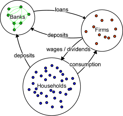
Figure 1: Schematic overview of the model structure showing the three agent types (banks, firms, and households), and their interactions. Firms pay dividends to their owners, and wages (financed through income and loans) to their workers. Households consume goods produced by the firms. Households and firms deposit money in banks, banks grant loans to the firms.

To test the economic and financial implications of the SRT we use the CRISIS macro-financial model. This is an economic simulator that combines a well-studied macroeconomic ABM (Gaffeo et al., 2008; Delli Gatti et al., 2008, 2011) with an ABM of financial markets. We use a modified version of the macroeconomic model of Delli Gatti et al. (2011), which additionally has an interbank market and is a closed, stock-flow consistent economic system that allows no in- or out-flows of cash. Here we give a short description of the model, for a comprehensive description, see Delli Gatti et al. (2011) or Gualdi et al. (2015) and for the modifications, see appendix A.

In the model, there are three types of agents: households, banks, and firms, as depicted in fig. 1. The agents interact on four different markets:

1. Firms and banks interact on the credit market.

2. Banks interact with banks on the interbank market.

3. Households and firms interact on the job market.

4. Households and firms interact on the consumption goods market.

Banks hold all firms’ and households’ cash as deposits. Households are randomly assigned as owners of firms and banks (share-holders). Agents repeat the following sequence of decisions at each time step:

1. firms define labour and capital demand,

2. banks raise liquidity for loans,

3. firms allocate capital for production (labour),

4. households receive wages, decide on consumption and saving,

5. firms and banks pay dividends, firms with negative liquidity go bankrupt,

6. banks and firms repay loans,

7. banks raise additional liquidity to manage unanticipated cash needs.

Households owning firms or banks receive dividends as income. All other households earn salaries for work done for firms. Banks and firms pay $20\%$ of their profits as dividends.

III.1 The agents

We give a short description of the agents; for more details on the agents and their interactions, see Delli Gatti et al. (2011), Gualdi et al. (2015), and appendix A.

III.1.1 Households

There are $H$ households of which there exist two types: firm owners, and workers. Each of them has a personal account $A_{j,b}(t)$ at one of the $B$ banks. $j$ indexes the worker, $b$ the bank. Household accounts are randomly assigned to banks. Workers apply for jobs at the $F$ different firms. If hired, they receive a fixed income $w$ per time step, and supply a fixed labour productivity $\alpha$. Firm owners receive their income through dividends from their firm’s profits. At each time step every household spends a fixed percentage $c$ of its current deposit account on the consumption market. Households compare prices of consumption goods from $z$ randomly chosen firms and buy the cheapest.

III.1.2 Firms

There are $F$ firms producing perfectly substitutable consumption goods. At every time step $t$ firms compute an expected demand for the next time step $D_{i}(t+1)$, and an estimated price $P_{i}(t+1)$ (subscripts label the firm), based on a rule that takes into account both excess demand/supply and the deviation of the price $P_{i}(t)$ from the average price at the present time step. Each firm computes the number of required workers to supply the expected demand. If the wages for the respective workforce exceed the firm’s current liquidity, it applies for a loan. Firms approach $n$ randomly chosen banks and choose the loan with the most favourable rate. If this rate exceeds a threshold rate $r^{\rm max}$, the firm only asks for $\phi$ percent of whatever loan was originally requested. Based on the outcome of this loan request, firms re-evaluate the required workforce, and hire or fire the necessary number of workers. Firms sell the goods on the consumption goods market. Firms go bankrupt if they have negative liquidity after the goods market has closed. Each of the bankrupted firm’s debtors (banks) incurs a capital loss in proportion to their investment in the company. Firm owners of bankrupted firms are personally liable, and their personal account is divided by the debtors pro rata. They immediately (next time step) start a new company. Their initial estimates for $D_{i}(t+1)$ and $P_{i}(t+1)$ equals the respective current averages in the population.

III.1.3 Banks

There are $B$ banks that offer firm loans at rates that take into account the individual specificity of banks (modelled by a uniformly distributed random variable), and the firms’ creditworthiness quantified by their leverage ratio (see appendix A). Firms pay a credit risk premium according to their creditworthiness, which is modelled by a monotonically increasing function of their financial fragility. Banks try to provide requested loans and grant them if they have enough liquid resources. If they do not have enough cash, they approach other banks in the interbank market to obtain the necessary amount. If a bank does not have enough cash and cannot raise the full amount for the requested firm loan on the interbank market it does not pay out the loan. Interbank and firm loans have the same duration. Additional refinancing costs of banks remain with the firms. Each time step firms and banks repay $\tau$ percent of their outstanding debt (principal plus interest). If banks have excess liquidity they offer it on the interbank market for a nominal interest rate. The interbank market is modelled after an electronic marketplace where, in principle, all participants can enter into business relationships. In the model, banks choose the interbank offer with the most favourable rate. This does not mean that the emerging interbank network is fully connected. Emerging interbank networks are shown in fig. 2 and (weighted) degree distributions can be found in fig. 7. Interbank rates $r_{ij}(t)$ offered by bank $i$ to bank $j$ take into account the specificity of bank $i$, and the creditworthiness (leverage ratio) of bank $j$. If a firm goes bankrupt the respective creditor bank writes off the respective outstanding loans as defaulted credits. If the bank does not have enough equity capital to cover these losses, it defaults. Following a bank default an iterative default-event unfolds for all interbank creditors. This may trigger a cascade of bank defaults. For simplicity’s sake, we assume no recovery for interbank loans. This assumption is reasonable in practice for short term liquidity (Cont et al., 2013). A cascade of bankruptcies happens within one time step. After the last bankruptcy is taken care of the simulation is stopped.

III.2 Implementation of the systemic risk tax and the Tobin tax

A systemic risk premium, in form of the SRT, is imposed on all interbank transactions. Before entering a desired loan contract ${l}_{ijk}(t)$, the credit seeking banks $i$ can get quotes for the $SRT^{(+k)}_{ij}(t)$ rates from the central bank, for various offering banks $j$. They choose the interbank offer from bank $j$ with the smallest total rate, which is composed of $r^{\rm total}_{ij}(t)=r_{ij}(t)+SRT^{(+k)}_{ij}(t)$. All other transactions are exempted from the SRT. In contrast to current market practice, the effective interest rate reflects both the creditworthiness of the borrowing counterparty and the SR increase associated with each transaction. The SRT is collected in a bailout fund. The SRT is calculated according to eq. 5. We approximate $p_{i}(t)$ by the financial fragility, defined by the borrower’s leverage at time $t$. For more details, see section A.2.

For comparison, we implement a Tobin-like (Tobin, 1978) FTT for interbank loans. We impose a constant tax rate of 0.2% of the transaction (this is about 5% of the interbank interest rates) on all interbank rates on offer. Other transactions are not taxed. The FTT makes lending less attractive for firms that borrow from banks requiring liquidity from the interbank market, as refinancing costs remain with the firms.

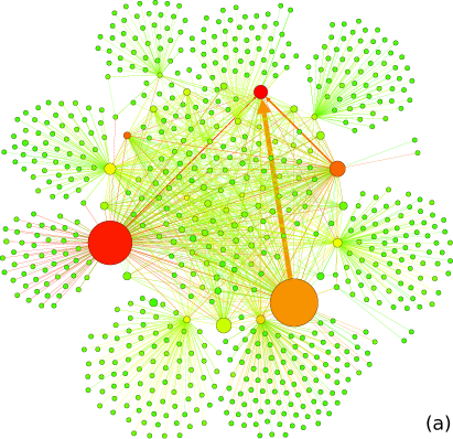
Figure 2: Banking network. (a) Austrian interbank network at the end of the first quarter of 2006, (b) the $20$ largest banks of the Austrian interbank network only, (c) banking network of the ABM without a tax, (d) with the FTT, and (e) with the SRT. Nodes (banks) are coloured according to their systemic importance $R_{i}$, from systemically important banks (red) to unimportant ones (green). The node-size represents the capitalisation of the banks. Width of the links are the liabilities of the banks in the interbank network and the colour is according to the source.

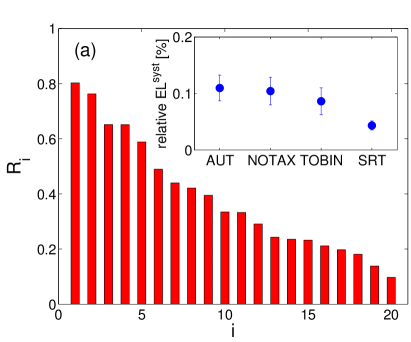
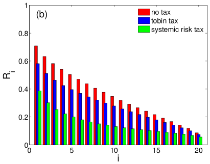
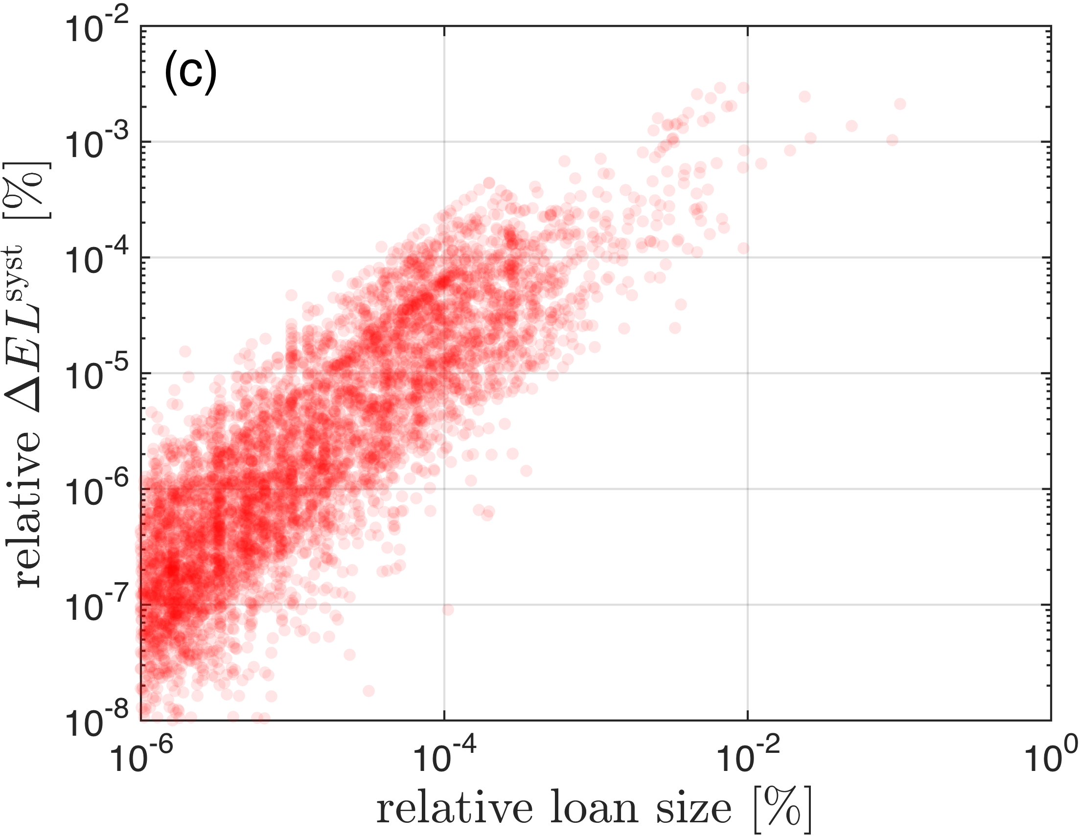
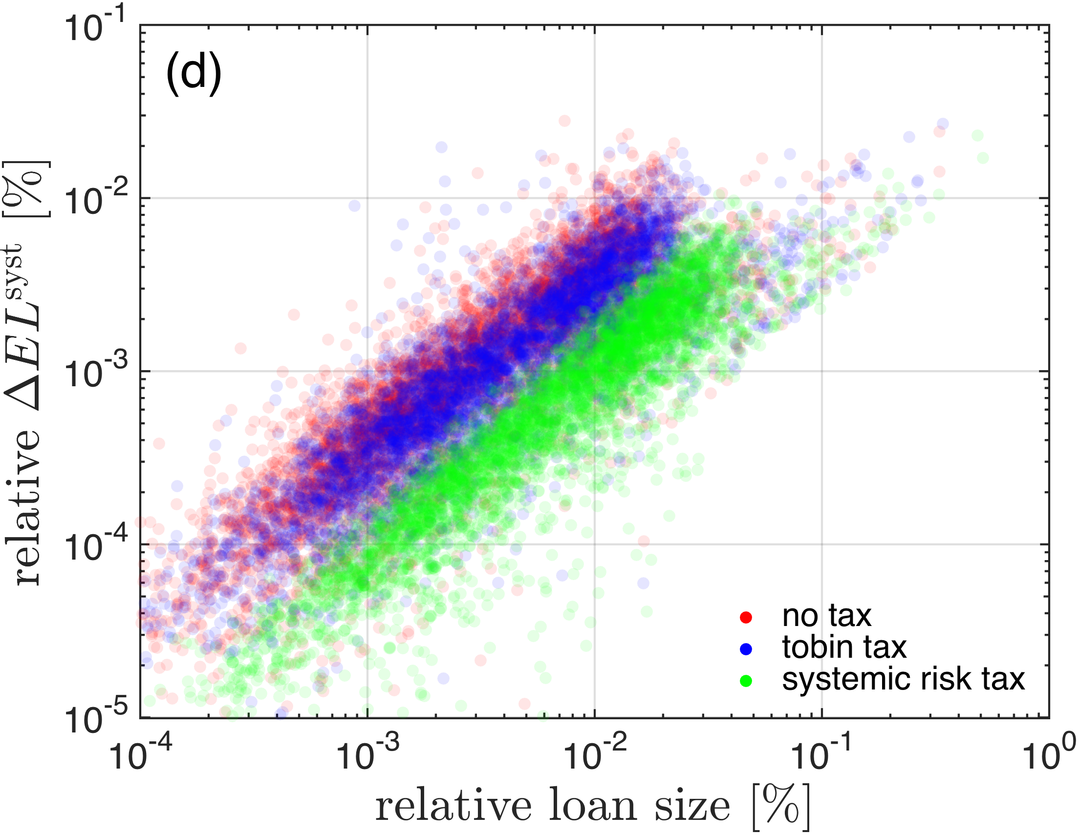
Figure 3: Expected systemic loss as measured by DebtRank, $EL^{\rm syst}_{i}\propto R_{i}$. (a) DebtRank, $R_{i}$ of the $20$ largest banks of the Austrian banking sector at the end of the first quarter of 2006. Banks are ordered by DebtRank, the most important being to the very left. Inset: Expected systemic loss from all banks for the Austrian interbank data and the three model modes. Here the SR measure is the size of a potential loss for the entire economy times the probability of that loss occurring as defined in eq. 3. (b) Model results for $R_{i}$: without a tax (red), with the FTT (blue), and with the SRT (green). Clearly, the SRT drastically reduces the SR contributions of individual banks. The situation without tax resembles the empirical distribution. (c) Marginal contributions on expected systemic loss $\Delta^{(+mn)}EL^{\rm syst}$ of individual interbank liabilities $L_{mn}$ vs. the relative size of interbank loans in double logarithmic scale. Every data point represents an interbank liability $L^{\rm data}_{mn}$, see appendix C. The loan size captures the credit risk for lenders, whereas $\Delta^{(+mn)}EL^{\rm syst}$ is the SR of the liability. (d) Marginal contributions for the simulations in the three modes. The SRT reduces SR but leaves contract sizes unchanged.

IV Results

We implement the above model in MATLAB for $B=20$ banks, $F=100$ firms, and $H=1300$ households. The model is run in three modes, without any tax, with the SRT, and with a Tobin-like FTT. Results are averages over $10,000$ independent, identical simulations across $500$ time steps. We set $\zeta=0.02$ (see section II), and for the Tobin-like FTT we impose a constant tax rate of 0.2% of the transaction. For different tax rates for the Tobin-like FTT and an alternative mode in which the SRT is set to the true increase in SR associated with each transaction ($\zeta=1$), see appendix B. Additionally in appendix B there is a short discussion of the effect of the SRT on the network properties.

We compare model results to historical, anonymised, and linearly transformed interbank liability data provided by the Austrian Central Bank (OeNB), see appendix C. In fig. 2(a) we show a snapshot of the Austrian interbank network at the end of the first quarter of 2006. Nodes symbolise the banks of the Austrian banking system and links represent their lending relations (weighted by the liabilities). Nodes are coloured according to their systemic importance $R_{i}$, from systemically important banks (red) to unimportant ones (green). The node-size represents the capitalisation of banks and the width of the links symbolises the liabilities. In fig. 2(b) we show the $20$ largest banks of the Austrian interbank network. Clearly, the $20$ largest banks contribute most to overall SR (red and orange dots). Figure 2(c) shows results from the ABM without a tax, (d) with the FTT, and (e) with the SRT. The SRT effectively reduces the spreading of SR by preventing systemically important nodes from lending. This can be seen from the fact that there are only green links in fig. 2(e). In the snapshot of the Austrian interbank network and in the model without the SRT numerous red links are clearly visible. In fig. 3(a) we show SR as measured by DebtRank $R_{i}$. In particular, we show $R_{i}$ for the $20$ largest banks (according to total assets) of the Austrian banking sector at the end of the first quarter of 2006. Here we calculate $R_{i}$ from $L^{\rm data}_{ij}(t)$ (see appendix C), in fig. 3(b) we use the net liability network $L^{\rm net}_{ij}(t)$. Banks are ordered by their DebtRank, the systemically most important one is to the very left, the least important one to the very right. The ABM results for $R_{i}(t)$ are presented in fig. 3(b): without a tax (red), with the FTT (blue) and with the SRT (green). The shown distributions are averages over $10,000$ independent simulations. Clearly, the SRT drastically reduces the SR contributions of individual banks. The situation without tax resembles the empirical distribution remarkably well. In fig. 3(c) the marginal contributions on expected systemic loss from eq. 3 are presented for all individual interbank liabilities $L^{\rm data}_{mn}$, as a function of the relative size of interbank loans. Every data point represents a single interbank liability $L^{\rm data}_{mn}$ from bank $m$ to $n$. Interbank loans are themselves power-law distributed (not shown), which is known empirically (Boss et al., 2005). The loan size captures the credit risk for lenders, whereas $\Delta^{(+mn)}EL^{\rm syst}$ is the SR contribution of the liability. Figure 3(d) shows the corresponding marginal contributions for the ABM simulations for the three modes. It is clearly visible that the SRT reduces the SR contribution of liabilities by approximately an order of magnitude (note the log scale), but leaves contract-sizes practically unchanged.

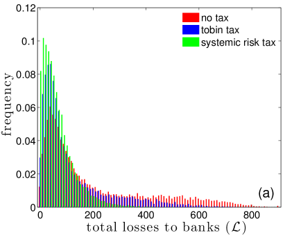
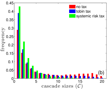
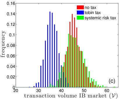
Figure 4: Comparison of no financial transaction tax (red) on interbank loans, with systemic risk tax (green), and Tobin tax (blue). (a) Distribution of total losses to banks ${\cal L}$, (b) distribution of cascade sizes ${\cal C}$ of defaulting banks, and (c) distribution of total transaction volume in the interbank market ${\cal V}$. $10,000$ independent, identical simulations, each with $500$ time steps, $20$ banks.

The effects of the SRT and the FTT on total losses to banks ${\cal L}$ (see appendix F) that occur as a consequence of bank defaults are shown in fig. 4(a). Clearly, the mode without tax (red) produces fat tails in the loss distributions of the banking sector. The Tobin tax slightly reduces losses. The SRT gets rid of big losses in the system completely (green). The remaining losses reflect those from firm defaults, which represents the economic risk in the system. Note that economic risk can hardly be managed. This elimination of losses on the interbank market is due to the fact that under the SRT the possibility for cascading defaults is drastically reduced. This is seen in fig. 4(b), where the distributions of cascade sizes $\mathcal{S}$ (see appendix F) for the three modes are compared. While the untaxed mode produces considerable cascade sizes of up to $20$ banks, the maximum cascade sizes under the SRT is less than half. The Tobin tax more or less follows the untaxed case. As mentioned above, the interbank loan sizes are practically unchanged under the SRT. This is also true for the total transaction volume $\mathcal{V}$ (see appendix F) in the interbank market, as can be seen in fig. 4(c), where the distributions of transaction volumes at time step 100 are shown. Obviously, the situation for the SRT (green) is very similar to the untaxed case (red), whereas the transaction volume is drastically reduced in the FTT scenario (blue), as expected.

V Discussion

We extend the notion of SR to individual liabilities within a financial network and show with empirical data of nation-wide interbank liabilities that this is indeed feasible. The notion of liability-specific SR allows us to quantify the marginal contribution of every financial transaction to overall SR. We propose a Pigovian tax (SRT) on every SR-increasing transaction, proportional to the marginal contribution to overall SR. By trying to avoid the SRT, financial institutions effectively rearrange the financial network over time, such that cascading failures can no longer occur. This process leads to a sustainable, self-organised and self-stabilising reduction of SR.

The notion of liability-specific SR is based on the probability of default and the impact of a failure of a financial institution, as measured by DebtRank. A central idea of this paper is to separate default risk from contagion risk. Contagion risk is the risk that a default by one institution leads to defaults of other institutions. DebtRank denotes the risk of financial contagion from the interbank liability network. The default risk of a financial institution depends on its financial condition and on the economic situation in general. In principle, it can also depend on financial networks, for example, the network of overlapping portfolios or the network of firms and regions or industries. However, if network contributions to the probability of default are small (second order), it becomes possible to separate default risk from contagion risk, as given by DebtRank, in a meaningful way. Otherwise, it is necessary to replace or generalise DebtRank with a methodology that includes the network of overlapping portfolios and other relevant networks.

In Poledna et al. (2015) we show that DebtRank and the ideas presented here can be generalised for multi-layer networks to quantify and reduce SR originating from different financial markets, such as derivatives, foreign exchange and securities. In future work we will conduct an empirical study on the network of overlapping portfolios and its implications for SR. Joint defaults can also be taken into account for example by copula methods. Once the default correlation has been estimated, it is possible to include the joint probability of default straightforwardly in the present framework. Joint defaults can be included by considering the joint probability of default of a group of financial institutions and by calculating the DebtRank for this group. Thus, additional terms containing the joint probability of default and the impact of a group can be added to eqs. 1 and 5.

We test the SRT within the framework of the CRISIS macro-financial model. The model produces SR-profiles of banks that are practically identical to those of actual interbank liability data. Even on the level of individual transactions the model is fully compatible with the empirical data (see also (Poledna et al., 2015)). The SRT drastically reduces the probability of a financial collapse due to restructured liability networks that minimise the size of cascading failure. The tax is implemented in a simple way: an agent would like to make a transaction (with a given counterparty) and expresses this interest by announcing it (and the envisioned counterparty) to the central bank. The latter computes the SR increase associated with the transaction based on the knowledge of the present state of the entire liability network and the capitalisation of its agents. The SR-increase is then presented to the agent as a tax (SRT) for that particular transaction. If the SR-increase is zero, then it is tax-free. The agent can now look for other counterparties to carry out exactly the same transaction. The agent will therefore typically screen several possible counterparties and then decide on the one with the lowest tax. Once the agent decides to carry out the transaction, it is executed and the tax is paid to the central bank or the government.

We show explicitly that SR is, to a large extent, a network property. We show that the SRT is able to restructure financial liability networks without loss of transaction volume in the financial market. For an explicit comparison we implement and test a Tobin-like tax that taxes all transactions regardless of their SR contributions. The Tobin-like tax does not restructure networks and only reduces SR because it also drastically reduces transaction volume in the system. This is damaging as it makes the system less efficient; the loss of efficiency materialises as expensive credit for the real economy. We tested an alternative mode in which the SRT is set to the true increase in SR associated with the transaction, and not only a fraction ($\zeta=1$). This alternative leads to much more homogeneous SR-spreading across all agents, and makes the system even safer, see fig. 3(b) and fig. 6(d), however, it is done at the cost of much reduced transaction volume.

An obvious alternative to the SRT are bank taxes for SIFIs as recently suggested by several authors (Cooley et al., 2009; Acharya et al., 2012; Adrian and Brunnermeier, 2011; Markose et al., 2012; Acharya et al., 2013; Zlatić et al., 2014), or alternatively, to increase capital requirements for them by imposing SIFI surcharges as proposed in Basel III (Bank for International Settlements, 2010). An immediate problem of a bank tax or capital surcharges, compared to the SRT, is that financial institutions sometimes have no control over their systemic importance. For instance, in case of publicly traded securities, such as bonds, financial institutions have no authority to decide who holds them and thus no influence on their systemic importance. In recent work the effects of the Basel III regulation framework on SR has been studied in the same ABM environment (Poledna et al., 2016). Results indicate that capital surcharges for SIFIs can reduce SR, but must be larger than specified in Basel III to have a measurable impact, and thus cause a loss of efficiency.

We close with a remark on the policy relevance of the SRT. We think that the concept that network-related SR can be managed most efficiently by restructuring the underlying network topologies, is generally true. We further believe that the concept of the SRT as presented here is directly policy relevant. In particular, the incentive scheme introduced to internalise the externalities that lead to SR, can be directly transferred to banking regulation. Technically, the requirements for its implementation would include an electronic market run by a central bank or another central authority. This electronic market would work in the same way as an airline reservations system, i.e. by holding a quote for a limited amount of time. The computational requirements for central banks to compute the SRT for several thousand banks on a minute by minute basis is by today’s standards a technical triviality. Central banks would have to record transactions in real-time; this is done as a matter of course for several financial markets routinely, for instance at the Banco de México (Solorzano-Margain et al., 2013; Poledna et al., 2015). There are no privacy issues; obtaining information about the portfolios of other banks from the SRT quotes is impossible, in the same way as it is impossible to infer the entries of a real valued matrix from the eigenvector associated to the largest real eigenvalue. The problem that generally applies to any FTT – that it should be implemented globally to avoid free riding – also applies in the context of the SRT.

We finally stress that the current market practice of not pricing SR into transaction-costs effectively amounts to an implicit subsidy for those with the highest contribution to overall SR, and an effective tax on those with the lowest. In that sense, the SRT can be seen as an insurance premium that keeps the public neutral with respect to the SR that is introduced by the non-optimal liability networks.

Appendix A Details of the model

In this section we describe the extensions and modifications of the macroeconomic model of Delli Gatti et al. [2011]. The modifications include the implementation of an interbank market and a closed, stock-flow consistent economic system that allows no in- or out-flow of cash. The closed economic system is also discussed in Gualdi et al. [2015].

A.1 The credit market

There are $B$ banks that offer firm loans at rates that take the individual specificity of banks (modelled by a uniformly distributed random variable) and the firms’ creditworthiness into account. Firms pay a credit risk premium according to their creditworthiness that is modelled by a monotonically increasing function of their financial fragility. A firm’s financial fragility is defined as the ratio between the outstanding debt and the liquid financial resources of the firm [Delli Gatti et al., 2011]. Specifically the interest rate for firm $\kappa$, borrowing from bank $i$ is given by

$$r^{\kappa}_{i}(t)=\bar{r}(1+\chi_{i}(t)\mu(l_{\kappa}(t))\quad,$$ (6)

where $\bar{r}$ is a benchmark interest rate, $\chi_{i}(t)$ is the specificity of bank $i$ – modelled as random variations in its operating costs, strategy, etc. and captured by a uniformly distributed random variable on the interval $(0,1)$. $\mu(l_{\kappa}(t))$ is a proxy for the financial fragility of the borrower – modelled by a monotonically increasing function $\mu(\cdot)$ of the borrower’s debt to liquidity ratio $l_{\kappa}(t)$. The hyperbolic tangent is chosen for $\mu(\cdot)$.

A.2 The interbank market

Banks try to provide firm loans and grant them if they have enough liquidity. If they do not have enough cash, they approach other banks in the interbank market to obtain the required amount. If a bank does not have enough cash, and cannot raise the full amount for the requested firm loan on the interbank market, it does not pay out the loan. Interbank and firm loans have the same duration. Additional refinancing costs of banks remain with the firms. Each time step firms and banks repay $\tau$ percent of their outstanding debt. If banks have excess liquidity they offer it on the interbank market. The interbank market is modelled after an electronic marketplace where, in principle, all participants can enter into business relationships. In the model, banks choose the interbank offer with the most favourable rate. This does not mean that the emerging interbank network is fully connected. Emerging interbank networks are shown in fig. 2 and (weighted) degree distributions can be found in fig. 7. Interbank rates $r_{ij}(t)$ offered by bank $i$ to bank $j$ take into account the specificity of bank $i$ and the creditworthiness of bank $j$. Specifically the interest rate on the interbank market for bank $j$ borrowing from bank $i$ is given by

$$r_{ij}(t)=\bar{r}(1+\psi_{i}(t)\mu(l_{j}(t))\quad,$$ (7)

where $\bar{r}$ is a benchmark interest rate, $\psi_{i}(t)$ is the specificity of bank $i$, modelled as random variations in its operating costs, strategy, etc. and captured by a uniformly distributed random variable on the interval $(0,0.1)$. $\mu(l_{j}(t))$ is a proxy for the financial fragility of the borrower, modelled by a monotonically increasing function $\mu(\cdot)$ of the borrower’s leverage $l_{j}(t)$. As the monotonically increasing function again the hyperbolic tangent is chosen. Banks add the additional refinancing costs to the offered interest rate for firms. Therefore the interest rate for firm $\kappa$, borrowing from bank $i$, which requires additional liquidity from bank $j$ is given by

$$r^{\kappa}_{ij}(t)=r^{\kappa}_{i}(t)+\frac{l_{jik}(t)}{b_{\kappa}(t)}r_{ji}(t)=\\ =\bar{r}\left(1+\chi_{i}(t)\mu(l_{\kappa}(t))+\frac{l_{jik}(t)}{b_{\kappa}(t)}\psi_{j}(t)\mu(l_{i}(t))\right)\quad,$$ (8)

where $b_{\kappa}(t)$ is the firm loan and $l_{jik}(t)/b_{\kappa}(t)$ is the ratio between the interbank and the firm loan.

A.3 Implementation of the systemic risk tax and the Tobin tax

A systemic risk premium, in form of the SRT, is imposed on all interbank transactions. Before entering a desired loan ${l}_{ijk}(t)$, the credit seeking banks $i$ can get quotes for the $SRT^{(+k)}_{ij}(t)$ rates from the central bank, for various banks $j$. They choose the interbank offer from bank $j$ with the smallest total rate, which is composed of $r^{\rm total}_{ij}(t)=r_{ij}(t)+SRT^{(+k)}_{ij}(t)$. All other transactions are exempted from the SRT. In contrast to current market practice, the effective interest rate reflects both the creditworthiness of the borrowing counterparty and the SR increase associated with each transaction. The SRT is collected in a bailout fund. The SRT from the main text is given by

$$SRT_{ij}^{(+k)}(t)=\zeta\max\\ \left[0,\sum_{i}p_{i}(t)\left(V^{(+k)}(t)R^{(+k)}_{i}(t)-V(t)R_{i}(t)\right)\right]\quad.$$ (9)

For $p_{i}(t)$ we use a proxy for the financial fragility of the borrower, modelled by a monotonically increasing function $p_{i}(t)=0.01\mu(l_{i}(t))$ of the borrower’s leverage $l_{i}(t)$ at time $t$.

For comparison we implement a FTT (Tobin tax [Tobin, 1978]) for interbank loans. We impose a constant tax rate of 0.2% of the transaction (this is about 5% of the interbank interest rates) on all interbank rates on offer. Other transactions are not taxed. The FTT makes lending less attractive for firms that borrow from banks requiring liquidity from the interbank market, as refinancing costs remain with the firms.

Interbank rates $r_{ij}(t)$ offered by bank $i$ to bank $j$ including the FFT or the SRT are composed of

$$r^{\rm total}_{ij}(t)=r_{ij}(t)+TAX\quad.$$ (10)

In case of the FFT the tax term is simply a constant tax rate of 0.2%

$$r^{\rm total}_{ij}(t)=r_{ij}(t)+0.002\quad.$$ (11)

To obtain a tax rate, the SRT must be expressed as a ratio with respect to the interbank loan ($SRT^{(+k)}_{ij}(t)/l_{jik}(t)$). The total rate is then given by

$$r^{\rm total}_{ij}(t)=r_{ij}(t)+\frac{SRT_{ij}^{(+k)}(t)}{l_{ijk}(t)}\quad,$$ (12)

where $r_{ij}(t)$ is from eq. 7. Banks add the additional refinancing costs, including taxes, to the offered interest rate for firms. Therefore eq. 6 becomes for the Tobin-like tax

$$r^{\kappa}_{ij}(t)=r^{\kappa}_{i}(t)+\frac{l_{jik}(t)}{b_{\kappa}(t)}r^{\rm total}_{ji}(t)=\\ =\bar{r}\left(1+\chi_{i}(t)\mu(l_{\kappa}(t))+\frac{l_{jik}(t)}{b_{\kappa}(t)}\psi_{j}(t)\mu(l_{i}(t))\right)+\\ +\frac{l_{jik}(t)}{b_{\kappa}(t)}0.002\quad,$$ (13)

and in case of the SRT,

$$r^{\kappa}_{ij}(t)=r^{\kappa}_{i}(t)+\frac{l_{jik}(t)}{b_{\kappa}(t)}r^{\rm total}_{ji}(t)=\\ =\bar{r}\left(1+\chi_{i}(t)\mu(l_{\kappa}(t))+\frac{l_{jik}(t)}{b_{\kappa}(t)}\psi_{j}(t)\mu(l_{i}(t))\right)+\\ +\frac{SRT_{ji}^{(+k)}(t)}{b_{\kappa}(t)}\quad.$$ (14)

A.4 Model parameters

All parameters of the model are collected in table 1.

Table 1: List of the parameters as used in the model.

number of banks	$B=20$
number of firms/capitalists	$F=100$
number of workers (households)	$H=1300$
share of dividends	$div=0.2$
general refinancing rate	$\bar{r}=0.02$
labour productivity	$\alpha=0.1$
credit demand contraction	$\phi=0.8$
rate of debt reimbursement	$\tau=0.05$
wage rate	$wb=1$
number of applications in consumption goods market	$z=2$
propensity to consume	$c=0.8$
number of applications in credit market	$n=5$

Appendix B Comparison of different tax rates for the Tobin-like financial transaction tax

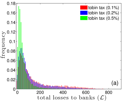
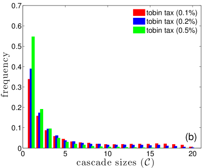
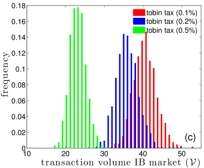
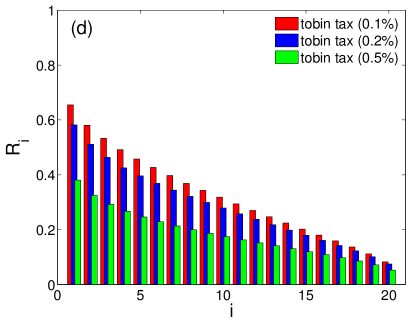
Figure 5: Comparison of different tax rates for the Tobin-like financial transaction tax, 0.1% (red), 0.2% (blue) and 0.5% (green). (a) Distribution of total losses to banks ${\cal L}$, (b) distribution of cascade sizes ${\cal C}$ of defaulting banks and (c) distribution of total transaction volume in the interbank market ${\cal V}$, (d) distribution of DebtRank $R_{i}$. Banks are ordered by DebtRank, the most important being to the very left. $10,000$ independent, identical simulations, each with $500$ time steps, $20$ banks.

In fig. 5 we show the distribution functions of the three measures for (a) losses ${\cal L}$, (b) cascade sizes ${\cal C}$, (c) transaction volume in the interbank market ${\cal V}$ and (d) the distribution of DebtRank $R_{i}$, for the simulations performed with different tax rates for the Tobin-like FTT, 0.1% (red), 0.2% (blue) and 0.5% (green). Clearly, the shape of the distribution of losses ${\cal L}$ and cascade sizes ${\cal C}$ are similar. The tail of the distributions is only reduced due to a decrease in efficiency (transaction volume), as can be seen in fig. 5(c). Evidently, average losses ${\cal L}$ are reduced at the cost of a loss of efficiency by roughly the same factor.

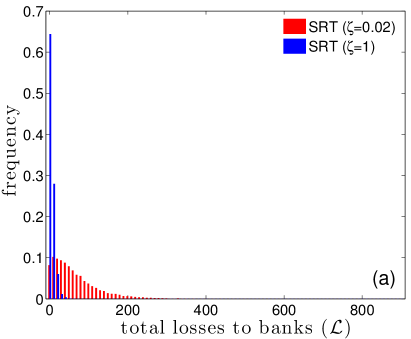
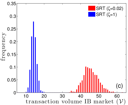
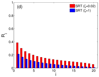
Figure 6: Comparison of different levels of the systemic risk tax, $\zeta=0.02$ (red) and $\zeta=1$ (blue). (a) Distribution of total losses to banks ${\cal L}$, (b) distribution of cascade sizes ${\cal C}$ of defaulting banks and (c) distribution of total transaction volume in the interbank market ${\cal V}$, (d) distribution of DebtRank $R_{i}$. Banks are ordered by DebtRank, the most important being to the very left. $10,000$ independent, identical simulations, each with $500$ time steps, $20$ banks.

For the comparison of different levels of the SRT we choose $\zeta=0.02$ (red) and $\zeta=1$ (blue), as shown in fig. 6. Again, we compare the three measures for (a) losses ${\cal L}$, (b) cascade sizes ${\cal C}$, (c) transaction volume in the interbank market ${\cal V}$ and (d) the distribution of DebtRank $R_{i}$. Clearly, for both $\zeta$ the SRT gets completely rid of big losses in the system. $\zeta=1$ reduces average losses ${\cal L}$ by a factor of $2$ compared to the case of $\zeta=0.02$, at the cost of a loss of efficiency by roughly the same factor, as can be seen in fig. 6(c). The SRT with ($\zeta=1$) leads to homogeneous SR spreading across all agents, as shown in fig. 6(d).

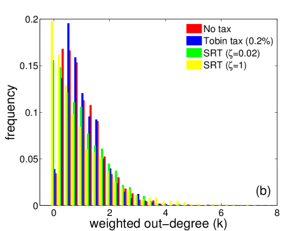
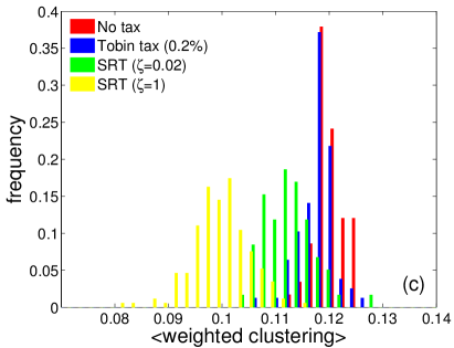
Figure 7: The effect of the bank selection process induced by the systemic risk tax on the interbank liability network topology. Distributions of weighted in-degrees $k$ (a), and weighted out-degrees $k$ (b) of the interbank liability network $(L^{\rm net}_{ij}(t))$, without FTT (red), 0.2% Tobin tax (blue), the SRT ($\zeta=0.02$) (green) and the SRT ($\zeta=1$) (yellow). (c) Shows the average weighted clustering coefficient of the interbank liability network $(L^{\rm net}_{ij}(t))$ from the model. The weighted in-degrees distributions are clearly affected in the SRT modes. The weighted out-degree distribution is mainly influenced by the cash needs of a bank. Therefore, the weighted out-degree distribution of the SRT modes is less clearly affected. The distributions are from an average over $1000$ simulations runs and show the situation at time $t=100$.

Table 2: Network measures

Mode	$\langle k\rangle$	$\langle k^{weighted}\rangle$	$\langle C_{i}\rangle$	$\langle C_{i}^{weighted}\rangle$	$\langle g_{i}\rangle$	$\langle g^{weighted}_{i}\rangle$
Normal	9.43(5)	38.4(35)	0.136(5)	0.119(3)	10.3(7)	40.2(53)
Tobin tax	9.39(9)	32.4(32)	0.135(5)	0.117(3)	10.4(7)	40.0(55)
SRT ($\zeta=0.02$)	9.15(13)	25.4(35)	0.138(6)	0.112(5)	11.9(20)	44.1(76)
SRT ($\zeta=1$)	8.73(20)	7.4(14)	0.122(6)	0.100(4)	11.3(12)	45.9(68)

In fig. 7 we show the effect of the bank selection process induced by the SRT on the interbank liability network topology. The distributions of weighted in-degrees $k$ of the interbank liability network $(L^{\rm net}_{ij}(t))$, without FTT (red), 0.2% Tobin tax (blue), the SRT ($\zeta=0.02$) (green) and, the SRT ($\zeta=1$) (yellow) are shown in fig. 7(a). Without FTT, the emerging liability network shows Poisson distributed in-degrees. The interbank network topology without FTT coincides nicely with the expected result from random linking. In the SRT modes, market participants looking for credit will try to avoid the tax by looking for credit opportunities that do not increase SR and are thus tax-free. This leads to fewer banks lending on the interbank market and is reflected in fig. 7(a) by the high number of nodes with a low weighted in-degree.

The total demand for interbank loans (which is approximately the same for the SRT with $\zeta=0.02$ as without FTT) is now serviced by fewer banks. As a result, the in-degree distribution of the SRT mode broadens and has a fat tail. The out-degree distribution is mainly influenced by the cash needs of a bank. Therefore, the weighted out-degree distribution of the SRT modes is less clearly affected, which is shown in fig. 7(b).

In fig. 7(c) we show the average weighted clustering coefficient of the interbank liability network $(L^{\rm net}_{ij}(t))$, without FTT (red), 0.2% Tobin tax (blue), the SRT ($\zeta=0.02$) (green) and the SRT ($\zeta=1$) (yellow). Average weighted clustering coefficients are calculated according to Barrat et al. [2004]. The average clustering is roughly the same without a FTT on interbank loans and for the 0.2% Tobin tax. The SRT reduces average clustering, as can be seen in fig. 7(c).

Mean values of various centrality measures, averaged over $1000$ simulations runs, can be found in table 2. $\langle k\rangle$ and $\langle k^{weighted}\rangle$ shows the mean degree and the weighted mean degree for the different modes. $\langle k\rangle$ is approximately the same for all modes. $\langle k^{weighted}\rangle$ shows the largest value for the normal mode and lower values in all other modes. Clearly, with the SRT ($\zeta=1$) $\langle k^{weighted}\rangle$ is substantially reduced. With $\langle C_{i}\rangle$ and $\langle C_{i}^{weighted}\rangle$ we show values for the average clustering coefficients and the average weighted clustering coefficients from fig. 7(c). Additionally, we provide values for the average betweenness centrality ($\langle g_{i}\rangle$) and the average weighted betweenness centrality ($\langle g^{weighted}_{i}\rangle$) for the different modes. The SRT increases both the $\langle g_{i}\rangle$ and the $\langle g^{weighted}_{i}\rangle$.

Appendix C Empirical data

Data provided by the Austrian Central Bank (OeNB) contains fully anonymised, and linearly transformed interbank liabilities/exposures $L^{\rm data}_{ij}(t)$ from the entire Austrian banking system, comprised of about 800 banks over 12 consecutive quarters from 2006-2008. The data set additionally includes total assets, total liabilities, assets due from banks, liabilities due to banks, and liquid assets (without interbank assets/liabilities) for all banks again in anonymised form. The data does not contain credit ratings of banks. Therefore we assume $p_{i}=0.0025$ for all banks in the data set. This corresponds approximately to Standard & Poor’s One-Year Global Corporate Default Rates for Rating Categories A+, A, and BBB+ in 2008 [Standard & Poor’s, 2009]. Representative Austrian banks are in the Rating Categories A+, A and A-.

Appendix D DebtRank

DebtRank is a recursive method suggested in Battiston et al. [2012a] to determine the systemic importance of nodes in financial networks. It is a number measuring the fraction of the total economic value in the network that is potentially affected by a node or a set of nodes. $L_{ij}$ denotes the interbank liability network at any given moment (loans of bank $j$ to bank $i$), and $C_{i}$ is the capital of bank $i$. If bank $i$ defaults and cannot repay its loans, bank $j$ loses the loans $L_{ij}$. If $j$ does not have enough capital available to cover the loss, $j$ also defaults. The impact of bank $i$ on bank $j$ (in case of a default of $i$) is therefore defined as

$$W_{ij}=\min\left[1,\frac{L_{ij}}{C_{j}}\right]\quad.$$ (15)

The value of the impact of bank $i$ on its neighbours is $I_{i}=\sum_{j}W_{ij}v_{j}$. The impact is measured by the economic value $v_{i}$ of bank $i$. For the economic value we use two different proxies. Given the total outstanding interbank liabilities of bank $i$, $L_{i}=\sum_{j}L_{ji}$, its economic value is defined as

$$v_{i}=L_{i}/\sum_{j}L_{j}\quad.$$ (16)

To take into account the impact of nodes at distance two and higher, this has to be computed recursively. If the network $W_{ij}$ contains cycles, the impact can exceed one. To avoid this problem an alternative was suggested in Battiston et al. [2012a], where two state variables, $h_{\rm i}(t)$ and $s_{\rm i}(t)$, are assigned to each node. $h_{\rm i}$ is a continuous variable between zero and one; $s_{\rm i}$ is a discrete state variable for three possible states, undistressed, distressed, and inactive, $s_{\rm i}\in\{U,D,I\}$. The initial conditions are $h_{i}(1)=\Psi\,,\forall i\in S;\;h_{i}(1)=0\,,\forall i\not\in S$, and $s_{i}(1)=D\,,\forall i\in S;\;s_{i}(1)=U\,,\forall i\not\in S$ (parameter $\Psi$ quantifies the initial level of distress: $\Psi\in[0,1]$, with $\Psi=1$ meaning default). The dynamics of $h_{i}$ is then specified by

$$h_{i}(t)=\min\left[1,h_{i}(t-1)+\sum_{j\mid s_{j}(t-1)=D}W_{ji}h_{j}(t-1)\right]\quad.$$ (17)

The sum extends over these $j$, for which $s_{j}(t-1)=D$,

$$s_{i}(t)=\begin{cases}D&\text{if }h_{i}(t)>0;s_{i}(t-1)\neq I,\\ I&\text{if }s_{i}(t-1)=D,\\ s_{i}(t-1)&\text{otherwise}\quad.\end{cases}$$ (18)

The DebtRank of the set $S$ (set of nodes in distress at time $1$), is $R^{\prime}_{S}=\sum_{j}h_{j}(T)v_{j}-\sum_{j}h_{j}(1)v_{j}$, and measures the distress in the system, excluding the initial distress. If $S$ is a single node, the DebtRank measures its systemic importance on the network. The DebtRank of $S$ containing only the single node $i$ is

$$R^{\prime}_{i}=\sum_{j}h_{j}(T)v_{j}-h_{i}(1)v_{i}\quad.$$ (19)

The DebtRank, as defined in eq. 19, excludes the loss generated directly by the default of the node itself and measures only the impact on the rest of the system through default contagion. For some purposes, however, it is useful to include the direct loss of a default of $i$ as well. The total loss caused by the set of nodes $S$ in distress at time $1$, including the initial distress is

$$R_{S}=\sum_{j}h_{j}(T)v_{j}\quad.$$ (20)

Appendix E Derivation of the expected systemic loss

To compute the expected systemic loss, we first consider the simple case where only one bank $i$ can default and all other $b-1$ banks survive. In this case the expected loss is given by ${\rm EL}_{i}^{\rm syst}({\rm one\,\,default})=V\cdot p_{i}\cdot(1-p_{1})\cdot\ldots\cdot(1-p_{i-1})\cdot(1-p_{i+1})\cdot\ldots\cdot(1-p_{b})\cdot R_{i}$, where $p_{i}$ is the probability of default of bank $i$, and $(1-p_{j})$ the survival probability of $j$. The general case occurs when we also consider possible joint defaults, meaning that a set of banks $S$ go into distress. Taking into account all possible combinations of defaulting and surviving banks, we arrive at a combinatorial expression of the expected loss for an economy of $b$ banks

$${\rm EL}^{\rm syst}=V\sum_{S\in\mathcal{P}(B)}\prod_{i\in S}p_{i}\prod_{j\in B\setminus S}(1-p_{j})\>R_{S}\quad,$$ (21)

where $\mathcal{P}(B)$ is the power set of the set of banks $B$, and $R_{S}$ is the DebtRank of the set $S$ of nodes initially in distress. $R_{\emptyset}$, the DebtRank of the empty set is defined as zero. The reason is that, by definition of DebtRank, $R_{S}\leq 1$, the value obtained in eq. 21 cannot exceed the total economic value.

Equation 21 is only practical for situations with less than about $20-30$ banks. Computing the power set and calculating DebtRanks for all possible combinations of more than $30$ banks in a large financial networks is practically unfeasible. If the default probabilities are low ($p_{i}\ll 1$) or the interconnectedness is low ($R_{i}\approx v_{i}$), $R_{S}$ can be approximated by

$$R_{S}\approx\sum_{i\in S}R_{i}\quad.$$ (22)

In an unconnected or unleveraged financial system ($R_{i}=v_{i}$), $R_{S}$ is exactly equal to $\sum_{i\in S}R_{i}$. If $p_{i}\ll 1$, the first terms of eq. 21 (with only one node initially in distress) contribute more to the final result. Thus the approximation eq. 22 has only a minor impact on the final result. Typically, $p_{i}\ll 1$ or $R_{i}\approx v_{i}$ holds in real word financial networks. With the approximation eq. 22, eq. 1 can be derived from eq. 21 by

$${\rm EL}^{\rm syst}\approx V\sum_{S\in\mathcal{P}(B)}\prod_{i\in S}p_{i}\prod_{j\in B\setminus S}(1-p_{j})\left(\sum_{i\in S}R_{i}\right)$$ (23)

$$=V\sum_{i=1}^{B}\underbrace{\left(\sum_{J\in\mathcal{P}(B\setminus\{i\})}\prod_{j\in J}p_{j}\prod_{k\in B\setminus(J\cup\{i\})}(1-p_{k})\right)}_{=1}p_{i}\,R_{i}$$ (24)

$$=V\sum_{i=1}^{B}p_{i}\,R_{i}\quad.$$ (25)

The term in brackets in eq. 24 sums to 1 (proof by induction). This approximation is practical for large financial networks, for details see [Poledna et al., 2015].

Appendix F Measures for losses, default cascades and transaction volume

We use the following three observables: (1) the size of the cascade, ${\cal C}$ as the number of defaulting banks triggered by an initial bank default ($1\leq{\cal C}\leq B$), (2) the total losses to banks following a default or cascade of defaults, ${\cal L}=\sum_{i\in I}\sum_{j=1}^{B}L_{ij}(t)$, where $I$ is the set of defaulting banks, and (3) the average transaction volume in the interbank market in simulation runs longer than $100$ time steps,

$$\mathcal{V}=\frac{1}{T}\sum_{t=1}^{T}\sum_{j=1}^{B}\sum_{i=1}^{B}\sum_{k\in K}l_{jik}(t)\quad,$$ (26)

where $K$ represents new interbank loans at time step $t$.

References

- The Economist [2013] The Economist. What Angela isn’t saying, August 2013.
- The Economist [2007a] The Economist. America’s vulnerable economy, November 2007a.
- The Economist [2007b] The Economist. CSI: credit crunch, October 2007b.
- Klimek et al. [2015] P. Klimek, S. Poledna, J.D. Farmer, and S. Thurner. To bail-out or to bail-in? answers from an agent-based model. Journal of Economic Dynamics and Control, 50:144–154, 2015.
- Tobin [1978] James Tobin. A proposal for international monetary reform. Technical Report 506, Cowles Foundation for Research in Economics, Yale University, 1978.
- Summers and Summers [1989] L. H. Summers and V. P. Summers. When financial markets work too well: A cautious case for a securities transactions tax. Technical Report 12, Columbia - Center for Futures Markets, 1989.
- McCulloch and Pacillo [2011] Neil McCulloch and Grazia Pacillo. The tobin tax a review of the evidence. Technical Report 1611, Department of Economics, University of Sussex, Jan 2011.
- Matheson [2012] Thornton Matheson. Security transaction taxes: issues and evidence. International Tax and Public Finance, 19(6):884–912, 2012.
- Aikman et al. [2013] D. Aikman, A. G. Haldane, and S. Kapadia. Operationalising a macroprudential regime: Goals, tools and open issues. Financial Stability Journal of the Bank of Spain, 24, 2013.
- Bank of England [2011] Bank of England. Instruments of macroprudential policy. Technical report, Bank of England, 2011.
- Bank of England [2013] Bank of England. The financial policy committee’s powers to supplement capital requirements: a draft policy statement. Technical report, Bank of England, 2013.
- Bank for International Settlements [2010] Bank for International Settlements. Basel III: A global regulatory framework for more resilient banks and banking systems. Bank for International Settlements, 2010.
- Georg [2011] Co-Pierre Georg. Basel III and systemic risk regulation - what way forward? Technical Report 17, Working Papers on Global Financial Markets, 2011.
- Duffie and Singleton [2012] D. Duffie and K.J. Singleton. Credit Risk: Pricing, Measurement, and Management. Princeton Series in Finance. Princeton University Press, 2012. ISBN 9781400829170.
- Bank for International Settlements [1988] Bank for International Settlements. International convergence of capital measurement and capital standards. Bank for International Settlements, Basel, 1988.
- Bank for International Settlements [2006] Bank for International Settlements. International Convergence of Capital Measurement and Capital Standards: A Revised Framework Comprehensive Version. Bank for International Settlements, Basel, 2006.
- Balin [2008] Bryan J. Balin. Basel I, Basel II, and emerging markets: A nontechnical analysis. Available at SSRN 1477712, 2008.
- De Bandt and Hartmann [2000] Olivier De Bandt and Philipp Hartmann. Systemic risk: A survey. Technical report, CEPR Discussion Papers, 2000.
- Eisenberg and Noe [2001] Larry Eisenberg and Thomas H. Noe. Systemic risk in financial systems. Management Science, 47(2):236–249, 2001.
- Minsky [1992] Hyman P. Minsky. The financial instability hypothesis. The Jerome Levy Economics Institute Working Paper, 74, 1992.
- Fostel and Geanakoplos [2008] Ana Fostel and John Geanakoplos. Leverage cycles and the anxious economy. American Economic Review, 98(4):1211–44, 2008.
- Geanakoplos [2010] John Geanakoplos. The leverage cycle. In D. Acemoglu, K. Rogoff, and M. Woodford, editors, NBER Macro-economics Annual 2009, volume 24, page 165. University of Chicago Press, 2010.
- Adrian and Shin [2008] Tobias Adrian and Hyun S. Shin. Liquidity and leverage. Tech. Rep. 328, Federal Reserve Bank of New York, 2008.
- Brunnermeier and Pedersen [2009] Markus Brunnermeier and Lasse Pedersen. Market liquidity and funding liquidity. Review of Financial Studies, 22(6):2201–2238, 2009.
- Thurner et al. [2012] S. Thurner, J.D. Farmer, and J. Geanakoplos. Leverage causes fat tails and clustered volatility. Quantitative Finance, 12(5):695–707, 2012.
- Caccioli et al. [2012] Fabio Caccioli, Jean-Philippe Bouchaud, and J. Doyne Farmer. Impact-adjusted valuation and the criticality of leverage. Risk, 25(12), 2012.
- Poledna et al. [2014] Sebastian Poledna, Stefan Thurner, J. Doyne Farmer, and John Geanakoplos. Leverage-induced systemic risk under Basle II and other credit risk policies. Journal of Banking & Finance, 42:199–212, 2014.
- Aymanns and Farmer [2015] Christoph Aymanns and Doyne Farmer. The dynamics of the leverage cycle. Journal of Economic Dynamics and Control, 50:155–179, 2015.
- Caccioli et al. [2015] Fabio Caccioli, J Doyne Farmer, Nick Foti, and Daniel Rockmore. Overlapping portfolios, contagion, and financial stability. Journal of Economic Dynamics and Control, 51:50–63, 2015.
- Acharya et al. [2009] Viral Acharya, Lasse Pedersen, Thomas Philippon, and Matthew Richardson. Regulating systemic risk. Restoring financial stability: How to repair a failed system, pages 283–304, 2009.
- Davies and Tracey [2014] Richard Davies and Belinda Tracey. Too big to be efficient? the impact of implicit subsidies on estimates of scale economies for banks. Journal of Money, Credit and Banking, 46(s1):219–253, 2014.
- Acharya et al. [2012] Viral Acharya, Lasse Pedersen, Thomas Philippon, and Matthew Richardson. Measuring systemic risk. Technical report, CEPR Discussion Papers, 2012. Available at SSRN: http://ssrn.com/abstract=1573171.
- Acemoglu et al. [2013] Daron Acemoglu, Asuman Ozdaglar, and Alireza Tahbaz-Salehi. Systemic risk and stability in financial networks. Technical report, National Bureau of Economic Research, 2013.
- Masciandaro and Passarelli [2013] Donato Masciandaro and Francesco Passarelli. Financial systemic risk: Taxation or regulation? Journal of Banking & Finance, 37(2):587–596, 2013.
- Cooley et al. [2009] Thomas Cooley, Thomas Philippon, Viral Acharya, Lasse Pedersen, and Matthew Richardson. Regulating systemic risk. In Viral Acharya and Matthew P Richardson, editors, Restoring Financial Stability: How to Repair a Failed System, pages 277–303. John Wiley & Sons, 2009.
- Adrian and Brunnermeier [2011] Tobias Adrian and Markus Brunnermeier. Covar. Technical report, National Bureau of Economic Research, 2011.
- Markose et al. [2012] Sheri Markose, Simone Giansante, and Ali Rais Shaghaghi. ‘Too interconnected to fail’ financial network of US CDS market: Topological fragility and systemic risk. Journal of Economic Behavior & Organization, 83(3):627–646, 2012.
- Acharya et al. [2013] Viral Acharya, Lasse Pedersen, Thomas Philippon, and Matthew Richardson. Taxing systemic risk. In J.P. Fouque and J.A. Langsam, editors, Handbook on Systemic Risk, pages 226–246. Cambridge University Press, 2013. ISBN 9781107023437.
- Zlatić et al. [2014] Vinko Zlatić, Giampaolo Gabbi, and Hrvoje Abraham. Reduction of systemic risk by means of pigouvian taxation. arXiv preprint arXiv:1406.5817, 2014.
- Brownlees and Engle [2012] Christian T Brownlees and Robert F Engle. Volatility, correlation and tails for systemic risk measurement. Available at SSRN 1611229, 2012.
- Huang et al. [2012] Xin Huang, Hao Zhou, and Haibin Zhu. Systemic risk contributions. Journal of financial services research, 42(1-2):55–83, 2012.
- Battiston et al. [2012a] Stefano Battiston, Michelangelo Puliga, Rahul Kaushik, Paolo Tasca, and Guido Caldarelli. Debtrank: Too central to fail? financial networks, the FED and systemic risk. Scientific reports, 2(541), 2012a.
- Thurner and Poledna [2013] Stefan Thurner and Sebastian Poledna. Debtrank-transparency: Controlling systemic risk in financial networks. Scientific reports, 3(1888), 2013.
- Caballero [2012] J. Caballero. Banking crises and financial integration. IDB Working Paper Series No. IDB-WP-364, 2012.
- Billio et al. [2012] Monica Billio, Mila Getmansky, Andrew W Lo, and Loriana Pelizzon. Econometric measures of connectedness and systemic risk in the finance and insurance sectors. Journal of Financial Economics, 104(3):535–559, 2012.
- Minoiu et al. [2013] Camelia Minoiu, Chanhyun Kang, V. S. Subrahmanian, and Anamaria Berea. Does financial connectedness predict crises? Technical Report 13/267, International Monetary Fund, Dec 2013.
- Roukny et al. [2013] Tarik Roukny, Hugues Bersini, Hugues Pirotte, Guido Caldarelli, and Stefano Battiston. Default cascades in complex networks: Topology and systemic risk. Scientific Reports, 3(2759), 2013.
- Haldane and May [2011] Andrew G. Haldane and Robert M. May. Systemic risk in banking ecosystems. Nature, 469(7330):351–355, 2011.
- Upper and Worms [2002] Christian Upper and Andreas Worms. Estimating bilateral exposures in the german interbank market: Is there a danger of contagion? Technical Report 9, Deutsche Bundesbank, Research Centre, 2002.
- Boss et al. [2004] M. Boss, M. Summer, and S. Thurner. Contagion flow through banking networks. Lecture Notes in Computer Science, 3038:1070–1077, 2004.
- Boss et al. [2005] M. Boss, H. Elsinger, M. Summer, and S. Thurner. The network topology of the interbank market. Quantitative Finance, 4:677–684, 2005.
- Soramäki et al. [2007] Kimmo Soramäki, Morten L. Bech, Jeffrey Arnold, Robert J. Glass, and Walter E. Beyeler. The topology of interbank payment flows. Physica A: Statistical Mechanics and its Applications, 379(1):317–333, 2007.
- Cajueiro et al. [2009] Daniel O Cajueiro, Benjamin M Tabak, and Roberto FS Andrade. Fluctuations in interbank network dynamics. Physical Review E, 79(3), 2009.
- Bech and Atalay [2010] Morten L. Bech and Enghin Atalay. The topology of the federal funds market. Physica A: Statistical Mechanics and its Applications, 389(22):5223–5246, 2010.
- Martínez-Jaramillo et al. [2014] Serafín Martínez-Jaramillo, Biliana Alexandrova-Kabadjova, Bernardo Bravo-Benitez, and Juan Pablo Solórzano-Margain. An empirical study of the mexican banking system’s network and its implications for systemic risk. Journal of Economic Dynamics and Control, 40:242–265, 2014. ISSN 0165-1889.
- Iori et al. [2008] Giulia Iori, Giulia De Masi, Ovidiu Vasile Precup, Giampaolo Gabbi, and Guido Caldarelli. A network analysis of the italian overnight money market. Journal of Economic Dynamics and Control, 32(1):259–278, 2008.
- Kyriakopoulos et al. [2009] F. Kyriakopoulos, S. Thurner, C. Puhr, and S. W. Schmitz. Network and eigenvalue analysis of financial transaction networks. The European Physical Journal B - Condensed Matter and Complex Systems, 71(4):523–531, October 2009.
- Huang et al. [2013] Xuqing Huang, Irena Vodenska, Shlomo Havlin, and H. Eugene Stanley. Cascading failures in bi-partite graphs: Model for systemic risk propagation. Scientific reports, 3(1219), 2013.
- Delli Gatti et al. [2009] Domenico Delli Gatti, Mauro Gallegati, Bruce C Greenwald, Alberto Russo, and Joseph E Stiglitz. Business fluctuations and bankruptcy avalanches in an evolving network economy. Journal of Economic Interaction and Coordination, 4(2):195–212, 2009.
- Battiston et al. [2012b] Stefano Battiston, Domenico Delli Gatti, Mauro Gallegati, Bruce Greenwald, and Joseph E Stiglitz. Liaisons dangereuses: Increasing connectivity, risk sharing, and systemic risk. Journal of Economic Dynamics and Control, 36(8):1121–1141, 2012b.
- Tedeschi et al. [2012] Gabriele Tedeschi, Amin Mazloumian, Mauro Gallegati, and Dirk Helbing. Bankruptcy cascades in interbank markets. PloS one, 7(12):e52749, 2012.
- Gabbi et al. [2015] Giampaolo Gabbi, Giulia Iori, Saqib Jafarey, and James Porter. Financial regulations and bank credit to the real economy. Journal of Economic Dynamics and Control, 50:117–143, 2015.
- Poledna et al. [2015] Sebastian Poledna, José Luis Molina-Borboa, Serafín Martínez-Jaramillo, Marco van der Leij, and Stefan Thurner. The multi-layer network nature of systemic risk and its implications for the costs of financial crises. Journal of Financial Stability, 20:70–81, 2015.
- Hull [2012] John C Hull. Options, Futures, and Other Derivatives. Prentice Hall PTR, 2012. ISBN 9780132164948.
- Hull and White [2000] John C Hull and Alan D White. Valuing credit default swaps I: No counterparty default risk. The Journal of Derivatives, 8(1):29–40, 2000.
- Hull and White [2001] John C Hull and Alan D White. Valuing credit default swaps II: Modeling default correlations. The Journal of Derivatives, 8(3):12–21, 2001.
- Gaffeo et al. [2008] Edoardo Gaffeo, Domenico Delli Gatti, Saul Desiderio, and Mauro Gallegati. Adaptive microfoundations for emergent macroeconomics. Eastern Economic Journal, 34(4):441–463, 2008.
- Delli Gatti et al. [2008] D. Delli Gatti, E. Gaffeo, M. Gallegati, G. Giulioni, and A. Palestrini. Emergent Macroeconomics: An Agent-Based Approach to Business Fluctuations. New economic windows. Springer, 2008. ISBN 9788847007253.
- Delli Gatti et al. [2011] Domenico Delli Gatti, Saul Desiderio, Edoardo Gaffeo, Pasquale Cirillo, and Mauro Gallegati. Macroeconomics from the Bottom-up. Springer Milan, 2011.
- Gualdi et al. [2015] Stanislao Gualdi, Marco Tarzia, Francesco Zamponi, and Jean-Philippe Bouchaud. Tipping points in macroeconomic agent-based models. Journal of Economic Dynamics and Control, 50:29–61, 2015.
- Cont et al. [2013] Rama Cont, Amal Moussa, and Edson Santos. Network structure and systemic risk in banking systems. In Jean-Pierre Fouque and Joseph A Langsam, editors, Handbook of Systemic Risk, pages 327–368. Cambridge University Press, 2013.
- Poledna et al. [2016] Sebastian Poledna, Olaf Bochmann, and Stefan Thurner. Basel III capital surcharges for G-SIBs fail to control systemic risk and can cause pro-cyclical side effects. arXiv preprint arXiv:1602.03505, 2016.
- Solorzano-Margain et al. [2013] Juan Pablo Solorzano-Margain, Serafin Martinez-Jaramillo, and Fabrizio Lopez-Gallo. Financial contagion: Extending the exposures network of the mexican financial system. Computational Management Science, 10(2-3):125–155, 2013.
- Barrat et al. [2004] A. Barrat, M. Barthélemy, R. Pastor-Satorras, and A. Vespignani. The architecture of complex weighted networks. Proceedings of the National Academy of Sciences of the United States of America, 101(11):3747–3752, 03 2004.
- Standard & Poor’s [2009] Standard & Poor’s. Understanding Standard & Poor’s rating definitions, June 2009.