RADIO-CONTINUUM STUDY OF MCSNR J0536–7038 (DEM L249)

Abstract

We present a detailed radio-continuum study on Australia Telescope Compact Array (ATCA) observations of Large Magellanic Cloud (LMC) supernova remnant (SNR), MCSNR J0536–7038. This Type Ia SNR follows a horseshoe morphology, with a size 32 pc $\times$ 32 pc (1-pc uncertainty in each direction). It exhibits a radio spectrum $\alpha=-0.52\pm 0.07$ between $\lambda=73$ and 6 cm. We report detections of regions showing moderately high fractional polarisation at 6 cm, with a peak value of 71$\pm$25% and a mean fractional polarisation of 35$\pm$8%. We also estimate an average rotation measure across the remnant of –237 rad m^-2. The intrinsic magnetic field appears to be uniformly distributed, extending in the direction of the two brightened limbs of the remnant.

1 Introduction

Supernova and their remnants play a crucial role in the evolution and structure of the interstellar medium (ISM), as they are responsible for the creation and distribution of the heavier elements and the chemical enrichment of galaxies. The Large Magellanic Cloud (LMC) is a favourable environment for observing supernova remnants (SNRs), due to the relatively close proximity in which it is located (and in turn larger angular size), making it possible to resolve these objects (as 1 pc =  4^′′). One LMC SNR of particular interest is MCSNR J0536–7038, a Type Ia SNR that has prominent Fe emission in its core and is thought to be the result of a ‘prompt’ Type Ia event (Borkowski, Hendrick, & Reynolds, 2006; Maggi et al., 2014).

MCSNR J0536–7038 was originally observed by Davies et al. (1976) using the 48-in SRC Schimdt camera, who gave this object the association DEM L249. They estimate an optical diameter of 180^′′$\times$120^′′ making note that this object was very faint and had diffused emission. Mathewson et al. (1983) find an optical size of 162^′′$\times$129^′′ and an X-ray size of $\sim$120^′′, an integrated flux density at 408 MHz of 130 mJy and a radio spectral index of $\alpha=-0.53$. Mills et al. (1984) recorded an integrated flux density measurement at 843 MHz of 850 mJy, updating the spectral index to $\alpha=-0.52$. They also note a horseshoe morphology for which they state that approximately one third of SNRs greater than 30^′′ are. Fusco & Preite (1984) find an ambient density of 0.05 cm^-3, a shock temperature of 1.5 keV, an age of 6.5$\times$10³ years, total swept up mass of 55$M_{\odot}$ and a shock velocity of 1100 km s^-1. No pulsar was found at this position by Manchester, Damico, & Tuohy (1985) in their search for short period pulsars. Berkhuijsen (1986) measure a radio surface brightness of 20.5 W Hz^-1 m^-2 sr^-1 using the radio diameter of 30 pc and spectral index of $\alpha=-0.52$. Also measured was a X-ray surface brightness of 32.4 erg s^-1 pc^-2 using the X-ray extent of 39 pc. Chu & Kennicutt (1988) listed the OB association of 560 pc to LH66,69 and listed the source as population type II? (with ‘?’ indicating uncertain classification). They also made note that there was no detectable CO in the vicinity. Filipović et al. (1995) used the Parkes radio telescope and measured integrated flux densities of 25 mJy (4750 MHz) and 34 mJy (4850 MHz). Williams et al. (1999) listed an average brightness of 0.0010 cts s^-1 arc min^-2, an X-ray size of 5.2^′$\times$3.3^′ and stated that the category of this SNR was unclassified as it did not show an unambiguous detection in the ROSAT observations. Haberl & Pietsch (1999) recorded an extent of 29.7^′′ and gave this SNR the association HP[99] 1173. Urošević et al. (2005) included MCSNR J0536–7038 in their study of the $\Sigma$-D relationship. Using a diameter of 39 pc, an integrated flux density of 62 mJy at 1400 MHz (which was extrapolated from the values listed for $\alpha$ and S₃₆ by Filipović et al. (1998)) and a spectrum of $\alpha=-0.61$, they calculated the surface brightness of this SNR to be 2.0$\times$10^-21 W/M² Hz sr. Blair et al. (2006) record this SNR as a large faint optical shell SNR which is brighter on the eastern side of the shell. They make note that it may be a mixed morphology class, and that C_III is present in its spectra which may indicate that the SNR is on the near side of the LMC. Seok et al. (2008) estimated an integrated flux of 9 mJy (4800 MHz). An optical extent of 3.1^′$\times$2.3^′ was recorded by using the MCSNR Atlas as published by Williams (http://www.astro.uiuc.edu/projects/atlas/). Payne et al. (2008) spectroscopically confirmed nature of this SNR based on the [S ii]/H${\alpha}$ ratio. Desai et al. (2010) recorded an extent of 3.0^′$\times$2.0^′ and no detection of a YSO for this object nor association with the molecular clouds.

Here, we report on new radio-continuum observations of MCSNR J0536–7038. The observations, data reduction and imaging techniques are described in Section 2. The astrophysical interpretation of newly obtained moderate-resolution total intensity and polarimetric images in combination with the existing Magellanic Cloud Emission Line Survey (MCELS) images are discussed in Section 3.

2 Observations and reduction

We observed MCSNR J0536–7038 along with various other LMC SNRs via the ATCA on the 15^th and 16^th of November 2011, using the new Compact Array Broadband Backend (CABB) at array configuration EW367 and at wavelengths of 3 and 6 cm ($\nu$=9000 and 5500 MHz). Baselines formed with the $6^{\mathrm{th}}$ ATCA antenna were excluded, as the other five antennas were arranged in a compact configuration. The observations were carried out in the so called “snap-shot” mode, totaling $\sim$50 minutes of integration over a 14 hour period. PKS B1934-638 was used for flux density calibration and PKS B0530-727 was used for secondary (phase) calibration. The phase calibrator was observed twice every hour for a total 78 minutes over the whole observing session. The miriad (Sault, Teuben, & Wright, 1995) and karma (Gooch, 1995) software packages were used for reduction and analysis. More information on the observing procedure and other sources observed in this project can be found in Bozzetto et al. (2012a, b, c, d, 2013) and De Horta et al. (2012).

The CABB 2 GHz bandwidth is a 16 times improvement from the previous 128 MHz, and with the new higher data sampling has increased the sensitivity of the ATCA by a factor of 4. The 2 GHz bandwidth not only aids in high sensitivity observations, but also allows data to be split into channels which can then be used for measuring Faraday rotation across the entire bandwidth, at frequencies close enough that the n $\times$ 180^∘ambiguities prevalent when making an estimate between distant frequencies, are no longer an issue.

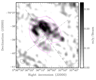
Fig. 1 : The top image shows the 3 cm intensity image of MCSNR J0536–7038  overlaid with 6 cm contours. The contours are 3, 6, 9 & 12$\sigma$ ($\sigma$ = 0.2 mJy/beam). The ellipse in the lower left corner represents the synthesised beamwidth at 3 cm of 22.4^′′$\times$15.7^′′. Also superimposed, are the major (NE–SW) and minor (SE–NW) axis. The middle and lower images show the intensity profile of the major and minor axis respectively, with an overlaid line at 3$\sigma$

Images were formed using miriad multi-frequency synthesis (Sault & Wieringa, 1994) and natural weighting. They were deconvolved with primary beam correction applied. The same procedure was used for both U and Q stokes parameter maps.

The 3 cm image (Fig. 1) has a resolution (full width half maximum (FWHM)) of 22.4^′′$\times$15.7^′′ (PA=44.5^∘) and an r.m.s noise of 0.1 mJy/beam. Similarly, we made an image of MCSNR J0536–7038 at 6 cm (seen as contours in Fig. 1) which has a FWHM of 38.5^′′$\times$24.2^′′ (PA=48.1^∘) and an estimated r.m.s. noise of 0.2 mJy/beam.

In addition to using our own observations, we measure the integrated flux density at several frequencies between $\lambda$ = 36 cm and 6 cm, and record these measurements along with previous measurements of this SNR in Table. 1. The 36 cm (843 MHz) measurements come from the Molonglo Synthesis Telescope (MOST; as described in Mills et al. 1984) and Sydney University Molonglo Sky Survey (SUMMS; Mauch et al. 2008) mosaic images. These 36 cm surveys are from two different sets of observations and we point that the MOST data comes with somewhat better uv coverage and sensitivity. This would be the most likely reason for a difference in flux density estimates (14 mJy or $\sim$20%) at this wavelength. The 20 cm (1384 MHz) measurement is from the mosaic image described in Hughes et al. (2007), while the 6 cm (4800 MHz) measurement comes from a mosaic image published by Dickel et al. (2010). Errors in these measurements predominately arose from defining the edge of the remnant. However, we estimate that the error in these measurements are in the order of 10%. Using these values from Table 1, we estimate a spectral index for MCSNR J0536–7038 of $\alpha=-0.52\pm 0.07$ (Fig. 2). We note the gap in flux density between our 6 cm (5500 MHz) measurement and the measurement from the 6 cm (4800 MHz) Dickel et al. (2010) mosaic. This can be explained by the missing short (zero) spacing measurement in interferometery, which is responsible for the large scale, extended emission. The shortest gap in our baseline array of 46 m affected the amount of flux observed, whereas the Dickel et al. (2010) mosaic incorporated a single dish (and therefore, zero-spacing) measurement from the Parkes radio telescope in addition to ATCA observations. Flux density measurements taken from our 3 cm image were omitted from the spectral index calculation as the effects from short spacing were far more detrimental than at 6 cm, as seen in Fig. 1. Measurements taken from the 3 cm Dickel et al. (2010) mosaic were also omitted as there was no reliable emission at the location of the remnant.

Table 1 : Integrated flux density measurements for MCSNR J0536–7038.

$\nu$	$\lambda$	r.m.s.	Beam Size	STotal	$\Delta$STotal	Reference
(MHz)	(cm)	(mJy/beam)	(′′)	(mJy)	(mJy)
408	73	40	157.2$\times$171.6	130	13	Mathewson et al. (1983)
843	36	—	46.4$\times$43.0	85	9	Mills et al. (1984)
843a	36	0.8	46.4$\times$43.0	70	7	This work
843b	36	1.0	47.3$\times$45.0	56	6	This work
1384	20	0.6	40	65	7	This work
4750	6	8	288	25	3	Filipović et al. (1995)
4800	6	—	35.0$\times$35.0	38	4	This work
4850	6	5	294	34	3	Filipović et al. (1995)
5000	6	—	258	34.5	3	Mathewson et al. (1983)c
5500	6	0.2	38.5$\times$24.2	24	2	This work

^aUses the MOST mosaic image.
^bUses the SUMMS mosaic image.
^cThis value was derived from the 408 MHz flux value from Mathewson et al. (1983) and their spectral index.

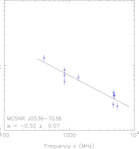
Fig. 2 : Radio spectrum of MCSNR J0536–7038

We also used the Magellanic Cloud Emission Line Survey (MCELS) that was carried out with the 0.6 m University of Michigan/CTIO Curtis Schmidt telescope, equipped with a SITE $2048\times 2048$ CCD, which gave a field of 1.35^∘ at a scale of 2.4^′′ pixel^-1. Both the LMC and SMC were mapped in narrow bands corresponding to H${\alpha}$, [O iii] ($\lambda$=5007 Å), and [S ii] ($\lambda$=6716, 6731 Å). All the data has been flux-calibrated and assembled into mosaic images, a small section of which is shown in Fig. 3. Further details regarding the MCELS are given by Pellegrini et al. (2012) and at http://www.ctio.noao.edu/mcels.

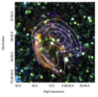
Fig. 3 : MCELS composite optical image (RGB =H$\alpha$,[Sii],[Oiii]) of MCSNR J0536–7038 overlaid with 6 cm contours. The contours are 3, 6, 9 and 12$\sigma$ ($\sigma$ = 0.2 mJy/beam)

3 Results and Discussion

MCSNR J0536–7038 exhibits a horseshoe morphology at 6 cm (Fig. 1) centered at RA (J2000) = 5^h 36^m 07^s.7, Dec (J2000) = –70^∘38^′20^′′. We selected a one-dimensional intensity profile across the approximate major (NE–SW) and minor (SE–NW) axes (Fig. 1) at the 3$\sigma$ noise level (0.6 mJy) to estimate the spatial extent of the remnant. Its size at 6 cm is 130^′′$\times$130^′′ with a 4^′′ uncertainty in each direction (32 $\times$ 32 pc with a 1 pc uncertainty in each direction at the LMC distance of 50 kpc (di Benedetto, 2008)). The remnant appears to be split into two limbs, the thicker, brighter limb toward the north-west and the thinner fainter limb towards the south-east.

The optical emission from the MCELS correlates nicely with our 6 cm radio-continuum emission. The [S ii] and H${\alpha}$ emission are quite similar, with rather uniform emission spread over the remnant but exhibiting brightening on the south-east limb. [O iii] emission is also found on this south-eastern limb (although thinner), however, unlike the H${\alpha}$ it is also found to show brightening towards the north-western limb. This is comparable to another LMC SNR that shares many similar properties (potential prompt Type Ia, older, opposite H${\alpha}$/[S ii] - [O iii]), MCSNR J0508–6902 (Bozzetto et al., 2014). The emission located towards the south-east of the remnant is a cluster of stars – NGC 2056 and not likely associated with this SNR.

There has already been an extensive X-ray study done for this SNR. However, we have overlaid 6 cm radio contours on a three colour composite Chandra image (Obs. ID: 3908) to show the association between the X-ray and radio-continuum emission (Fig. 4). We find that the radio-continuum emission loosely follows the low energy X-ray band (0.45–1.03 keV) and the medium band X-ray emission is confined in the interior of the remnant.

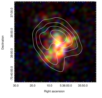
Fig. 4 : Chandra three colour composite (red: 0.45–1.03 keV, green: 1.03–1.32 keV, blue: 1.32–2.2 keV) of MCSNR J0536–7038 overlaid with 6 cm radio contours of 3 6 9 & 12$\sigma$ ($\sigma$ = 0.2 mJy)

The spectral energy distribution (SED) of the remnant between 36 cm and 6 cm ($\alpha=-0.52\pm 0.07$; based on the values in Table 1) shows the non-thermal nature of this remnant at radio-wavelengths. This value of $-0.5$ is typical spectral index of SNRs (Mathewson et al., 1983; Filipović et al., 1998).

As we are unable to create a reliable 3 cm polarisation image (due to this wavelength being significantly affected by missing short spacing), we instead make use of the wide 2 GHz bandwidth from the 6 cm observations in order to carry out a comparative polarisation study. The 2048 channels at 6 cm were split into two even parts, each consisting of 1024 channels. Both images were convolved to the same resolution so that they could be compared.

Fractional polarisation (P) was calculated for both 6 cm images using:

P = $\frac{\sqrt{S_{Q}^{2}+S_{U}^{2}}}{S_{I}}$

where $S_{Q},S_{U}$ and $S_{I}$ are integrated intensities for Q, U and I Stokes parameters. We estimate a mean fractional polarisation value of $P\cong$ 35 $\pm$ 8% at 6 cm. This relatively high level of polarisation is (theoretically) expected for an SNR with a radio spectrum of less than $-0.5$ (Rolfs & Wilson, 2003), which is in agreement with our spectral index of $\alpha\cong-0.52$. The structure of this polarisation can be seen in the top image of Fig. 5, where the electric field vectors at 6 cm have been superimposed on the 6 cm contours. These vectors are primarily facing the north-south direction, with slight change over the remnant, mostly found towards the norths and south limbs. We find a peak fractional polarisation for this SNR of $P=71$ $\pm$ 25%. This level of polarisation is comparatively higher than most LMC SNRs, and is on par with the peak value found for LMC SNR J0455–6838 by Crawford et al. (2008), of $\sim$70%.

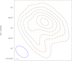
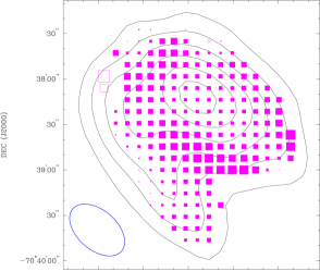
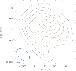
Fig. 5 : Top - electric field of MCSNR J0536–7038 at 6 cm. Middle - rotation measure, with filled boxes representing positive rotation and open boxes representing negative rotation. Bottom - Intrinsic magnetic field vectors with the polarised intensity based on 6 cm values. All images are overlaid with 6 cm contours of 3, 6, 9, 12, 15 & 18$\sigma$ ($\sigma$ = 2 mJy/beam). The ellipse in the lower left corner represents the synthesised beamwidth of 42.7^′′$\times$26.1^′′and the line directly below (in the top and bottom images) shows a polarisation vector of 100%

High levels of intrinsic fractional polarisation (with a maximum of $p=(3-3\alpha)/(5-3\alpha)$ = $\sim$70% in a ordered field) from synchrotron emission is possible, and we do expect the magnetic field components perpendicular to compression to be amplified. However, such levels of polarisation are not expected to be observed due to the non-uniform regions of the polarised emission in addition to instrumental depolarisation and/or physical depolarisation effects outside the SNR. A possible explanation for these high values is given in Dickel, Milne, & Strom (2000) where they pointed that the fractional polarisation can be artificially increased due to the polarised intensity having more fine scale structure than the total intensity, and therefore, the missing short spacing between antennas misrepresents the background level.

Polarisation position angles were taken from both 6 cm polarisation images and used to estimate Faraday rotation for this SNR. The rotation measure for this remnant can be seen in Fig. 5, where positive rotation measure is shown by filled boxes and negative rotation by empty boxes. The rotation measure is predominately positive across the remnant, with a few negative values found towards the edge of the remnant. However, the polarised intensity where these negative values are situated is too low to accurately determine rotation measure, and are therefore, probably not real. The average rotation measure across the remnant is 237 rad m^-2.

To see the intrinsic magnetic field of MCSNR J0536–7038, we first de-rotate the 6 cm electric field vectors to their zero-wavelength position angle, and then rotate the vectors by 90 degrees to get the perpendicular magnetic field. The result of this can be seen in Fig. 5, where we find the magnetic field vectors overlaid on 6 cm contours. The vectors appear uniform across the field, with slight deviations along the east side and a couple on the northern most line. However, all lie within the 10–20% of 6–9 $\sigma$ which makes them 1-2$\sigma$, and therefore not significant. The overall morphology suggests that MCSNR J0536–7038 went off in a region of uniformly NE–SW field and so compressed it more in the NW–SE direction.

From the position of MCSNR J0536–7038 at the surface brightness to diameter ($\Sigma$ - D) diagram ((D, $\Sigma$) = (32 pc, 3.6 $\times$ 10^-21 W m^-2 Hz^-1 sr^-1)) by Berezhko & Völk (2004), we can estimate that the remnant is likely to be an SNR in the late energy conserving phase, with an explosion energy between 0.25 and 1 $\times$ 10⁵¹ ergs, which evolves in an environment of density $\sim$1 cm^-3.

4 Conclusions

We provide a radio-continuum study of MCSNR J0536–7038, measuring an extent of 32 pc $\times$32 pc, strong polarisation across the remnant, with a mean of  35%, nice optical to radio association for the SNR. We also find the intrinsic magnetic field for this remnant, which uniformly follows the path of the compressed emission. We estimate a spectrum of $\alpha=-0.52$ between $\lambda$=6 cm & 36 cm, typical of a mid to older remnant. The rotation measure across the remnant is predominately positive with a mean rotation measure of –237 rad m^-2.

Acknowledgements

The Australia Telescope Compact Array is part of the Australia Telescope which is funded by the Commonwealth of Australia for operation as a National Facility managed by CSIRO. The MCELS is funded through the support of the Dean B. McLaughlin fund at the University of Michigan and through NSF grant 9540747. The scientific results reported in this article are based on observations made by the Chandra X-ray Observatory (CXO). We thank the referee for numerous helpful comments that have greatly improved the quality of this paper.

References

- Berezhko & Völk (2004) Berezhko E. G., Völk H. J., 2004, A&A, 427, 525
- Berkhuijsen (1986) Berkhuijsen, E. M., 1986, A&A, 166, 257
- Blair et al. (2006) Blair, W. P., Ghavamian, P., Sankrit, R. and Danforth, C. W., 2006, ApJS, 165, 480
- Borkowski, Hendrick, & Reynolds (2006) Borkowski, K. J., Hendrick, S. P., Reynolds, S. P. 2006, ApJ, 652, 1259
- Bozzetto et al. (2012a) Bozzetto L. M. et al., 2012a, MNRAS, 420, 2588
- Bozzetto et al. (2012b) Bozzetto L. M., Filipović M. D., Crawford E. J., Payne J. L., de Horta A. Y., Stupar M. 2012b, Rev. Mex. Astron. Astro s., 48, 41
- Bozzetto et al. (2012c) Bozzetto, L. M., Filipović, M. D., Crawford, E. J., De Horta, A. Y. and Stupar, M., 2012c, Serbian Astronomical Journal, 184, 69
- Bozzetto et al. (2012d) Bozzetto, L. M., Filipović, M. D., Urosevic, D. and Crawford, E. J., 2012d, Serbian Astronomical Journal, 185, 25
- Bozzetto et al. (2013) Bozzetto L. M., et al., 2013, MNRAS, 432, 2177
- Bozzetto et al. (2014) Bozzetto L. M., et al., 2014, arXiv:1401.1868
- Chu & Kennicutt (1988) Chu, Y.-H. and Kennicutt, Jr., R. C., 1988, AJ, 96, 1874
- Crawford et al. (2008) Crawford, E. J., Filipović, M. D., de Horta, A. Y., Stootman, F. H., Payne, J. L. 2008, SAJ, 177, 61
- Davies et al. (1976) Davies, R. D., Elliott, K. H. and Meaburn, J., 1976, MmRAS, 81, 89
- De Horta et al. (2012) De horta, A. Y., et al., 2012, A&A, 540, A25
- Desai et al. (2010) Desai, K. M., Chu, Y.-H., Gruendl, R. A., Dluger, W., Katz, M., Wong, T., Chen, C.-H. R., Looney, L. W., Hughes, A., Muller, E., Ott, J. and Pineda, J. L., 2010, AJ, 140, 584
- Dickel, Milne, & Strom (2000) Dickel, J. R., Milne, D. K. and Strom, R. G., 2000, ApJ, 543, 840
- Dickel et al. (2010) Dickel J. R., McIntyre V. J., Gruendl R. A., Milne D. K., 2010, AJ, 140, 1567
- di Benedetto (2008) di Benedetto G. P., 2008, MNRAS, 390, 1762
- Filipović et al. (1995) Filipović, M. D., Haynes, R. F., White, G. L., Jones, P. A., Klein, U., Wielebinski, R. 1995, A&AS, 111, 311
- Filipović et al. (1998) Filipović, M. D., Haynes, R. F., White, G. L., Jones, P. A., 1998, A&AS, 130, 421
- Fusco & Preite (1984) Fusco-Femiano, R. and Preite-Martinez, A., 1984, ApJ, 281, 593
- Gooch (1995) Gooch R., 1995, in Shaw R. A., Payne H. E., Hayes J. J. E., eds, ASP Conf. Ser. Vol. 77, Space and the Spaceball. Astron. Soc. Pac., San Francisco, p. 144
- Haberl & Pietsch (1999) Haberl, F. and Pietsch, W., 1999, A&AS, 139, 277
- Hughes et al. (2007) Hughes A., Staveley-Smith L., Kim S., Wolleben M., Filipović M., 2007, MNRAS, 382, 543
- Maggi et al. (2014) Maggi, P., Haberl, F., Kavanagh, P. J., Points, S. D., Dickel, J., Bozzetto, L. M., Sasaki, M., Chu, Y.-H., Gruendl, R. A., Filipović, M. D. and Pietsch, W., 2014, A&A, 561, 76
- Manchester, Damico, & Tuohy (1985) Manchester, R. N., Damico, N. and Tuohy, I. R., 1985, Mon. Not. R. Astron. Soc., 212, 975
- Mathewson et al. (1983) Mathewson, D. S., Ford, V. L., Dopita, M. A., Tuohy, I. R., Long, K. S., Helfand, D. J. 1983, ApJS, 51, 345
- Mauch et al. (2008) Mauch T., Murphy T., Buttery H. J., Curran J., Hunstead R. W., Piestrzynski B., Ropbertson J. G., Sadler E. M., 2008, VizieR Online Data Catalog, 8081, 0
- Mills et al. (1984) Mills B. Y., Turtle A. J., Little A. G., Durdin J. M., 1984, Aust. J. Phys., 37, 321
- Payne et al. (2008) Payne, J. L., White, G. L. and Filipović, M. D., 2008, MNRAS, 383, 1175
- Pellegrini et al. (2012) Pellegrini, E. W., Oey, M. S., Winkler, P. F., Points, S. D., Smith, R. C., Jaskot, A. E. and Zastrow, J., 2012, ApJ, 755, 40
- Rolfs & Wilson (2003) Rolfs, K., Wilson, T.: 2003: “Tools of Radio Astronomy 4ed.”, Springer, Berlin.
- Sault & Wieringa (1994) Sault R. J., Wieringa M. H. 1994, A&AS, 108, 585
- Sault, Teuben, & Wright (1995) Sault R. J., Teuben P. J., Wright M. C. H., 1995, in Shaw R. A., Payne H. E., Hayes J. J. E., eds, ASP Conf. Ser. Vol. 77, A Retrospective View of MIRIAD. p. 433
- Seok et al. (2008) Seok, J. Y., Koo, B.-C., Onaka, T., Ita, Y., Lee, H.-G., Lee, J.-J., Moon, D.-S., Sakon, I., Kaneda, H., Lee, H. M., Lee, M. G. and Kim, S. E., 2008, PASJ, 60, 453
- Urošević et al. (2005) Urošević, D., Pannuti, T. G., Duric, N. and Theodorou, A., 2005, A&A, 435, 437
- Williams et al. (1999) Williams, R. M., Chu, Y.-H., Dickel, J. R., Petre, R., Smith, R. C. and Tavarez, M., 1999, ApJS, 123, 467