Effect of one-, two-, and three-body atom loss processes on superpositions of phase states in Bose-Josephson junctions

Abstract

In a two-mode Bose-Josephson junction formed by a binary mixture of ultracold atoms, macroscopic superpositions of phase states are produced during the time evolution after a sudden quench to zero of the coupling amplitude. Using quantum trajectories and an exact diagonalization of the master equation, we study the effect of one-, two-, and three-body atom losses on the superpositions by analyzing separately the amount of quantum correlations in each subspace with fixed atom number. The quantum correlations useful for atom interferometry are estimated using the quantum Fisher information. We identify the choice of parameters leading to the largest Fisher information, thereby showing that, for all kinds of loss processes, quantum correlations can be partially protected from decoherence when the losses are strongly asymmetric in the two modes.

I Introduction

Non-classical states such as squeezed states and macroscopic superpositions of coherent states are particularly interesting for high-precision interferometry since they allow for phase resolution beyond the standard quantum limit. One of the systems where such states may be engineered is a Bose-Einstein condensate (BEC) made of metastable vapors of ultracold atoms. This system displays a wide tunability of parameters: the interaction between atoms can be controlled by Feshbach resonances fano1961 ; feshbach1958 , and, by using optical lattices, the BEC can be coherently split into up to few thousands sub-systems with controlled tunneling between them Bloch2005 ; Bloch2008 ; Weitenberg2011 . When the condensed atoms are trapped in a double-well potential, they realize an external Bose-Josephson junction (BJJ). The spatial wave functions localized inside a single well constitute the two modes of the BJJ and the tunneling between the wells leads to an inter-mode coupling. An internal BJJ is formed by condensed atoms in two hyperfine states resonantly coupled by a microwave radio-frequency field, trapped in a single harmonic well. In both cases, when inter-mode coupling dominates interactions, the ground state of the BJJ is a spin coherent state (CS), that is, a product state in which all atoms are in the same superposition of the two modes. After a sudden quench to zero of the coupling, the dynamical evolution builds up entangled states because of the interactions between atoms. In the absence of decoherence mechanisms, the system evolves first into squeezed states kitagawa1993 ; soerensen2001a ; soerensen2001 , then to multi-component superpositions of CSs yurke1986 ; stoler1971 , and then has a revival in the initial CS.

To date, only squeezed states, which appear at times much shorter than the revival time, have been realized experimentally esteve2008 ; riedel2010 ; gross2010 . At longer times, recombination and collision processes leading to losses of atoms in the BEC give rise to strong decoherence effects and eventually to the disappearance of the BEC. Particle losses also destroy partially the coherence of the squeezed states, as analyzed quantitatively in sinatra1998 ; yun2008 ; yun2009 ; pawlowskiBackground . The phase noise produced by magnetic fluctuations in internal BJJs is another important source of decoherence riedel2010 ; ferrini2010 . The superpositions of CSs appear later in the evolution and are expected to be more fragile than squeezed states. The main theoretical studies on decoherence effects on such superpositions have focused on the influence of the coupling of the atoms with the electromagnetic vacuum huang2006 and the impact of phase noise ferrini2010a . In particular, it has been shown in ferrini2010 ; ferrini2010a that the coherences of the superpositions are not strongly degraded by phase noise, and this degradation does not increase with the number of atoms in the BJJ. Under current experimental conditions, photon scattering is typically negligible and phase noise can be decreased by using a spin-echo technique gross2010 . In such conditions, the most important source of decoherence is particle losses. Three kinds of loss processes may play a role: one-body losses, due to inelastic collisions between trapped atoms and the background gas; two-body losses, resulting from scattering of two atoms in the magnetic trap, which changes their spin and gives them enough kinetic energy to be ejected from the trap; and three-body losses, where a three-body collision event produces a molecule and ejects a third atom out of the trap.

In a previous work pawlowski2013 , we have analyzed the impact of two-body losses on the superpositions of coherent states produced in internal BJJs. In this paper, we extend this analysis and study the combined effect of one-body, two-body, and three-body losses on the formation of the superposition states. By using a quantum trajectory approach we find, in agreement with Ref. sinatra2012 , that for all types of losses the fluctuations in the atomic interaction energy produced by the random loss events give rise to an effective phase noise. We show that for weak loss rates this noise is responsible for the strongest decoherence effect. The tunability of the scattering lengths by Feshbach resonances makes it possible to switch the effective phase noise off in the mode loosing more atoms, without changing the interaction strength in the unitary dynamics, i.e. keeping the formation times of the superpositions fixed. One may in this way partially protect the coherences of the superpositions for strongly asymmetric losses in the two modes, as it has been already pointed out in Ref. pawlowski2013 in the case of two-body losses. We show in this work that this result applies to all loss processes and that for moderate loss rates the corresponding states are more useful for high-precision atom interferometry than the squeezed states. This usefulness for interferometry is quantified by the quantum Fisher information $F$, which is related to the best phase precision achievable in one measurement according to $(\Delta\varphi)_{\text{best}}=1/\sqrt{F}$ braunstein1994 . We calculate the Fisher information as a function of time in the lossy BJJ by using an exact diagonalization of the master equation.

The paper is organized as follows. In Sec. II we recall the dynamical evolution in a BJJ in the absence of tunneling and present the theoretical tools used to analyze it. We first introduce the Bose-Hubbard model and the Markovian master equation describing the dynamics in the presence of particle losses (Sec. II.1). In the remaining part of the section, we give a brief account on atom interferometry (Sec. II.2) and on the quantum trajectory method for solving master equations (Sec. II.3). Our main results on the time evolution of the quantum Fisher information in a lossy BJJ are presented in Sec. III. These results are explained in Sec. IV with the help of the quantum trajectory approach. We analyze separately the contributions to the total atomic density matrix of quantum trajectories which do not experience any loss (Sec. IV.2) and of trajectories having a single or several loss events (Sec. IV.3). The various physical effects leading to an increase or a decrease of the Fisher information at the formation times of the macroscopic superpositions are described in detail (Sec. IV.4). Section V contains a summary and conclusive remarks. Four appendices offer some additional technical details.

II Model and methods

II.1 Quenched dynamics of a Bose-Josephson Junction

In this subsection we first recall the main features of the dynamics of a two-mode Bose-Josephson junction (BJJ) in the quantum regime after a sudden quench of the inter-mode coupling to zero. We then introduce the Markovian master equation describing atom losses in the BJJ and the conditional density matrices with fixed numbers of atoms.

II.1.1 Initial coherent state and Husimi distribution

We denote by $\hat{a}_{i}$, $\hat{a}_{i}^{\dagger}$, and $\hat{n}_{i}=\hat{a}_{i}^{\dagger}\hat{a}_{i}$ the bosonic annihilation, creation, and number operators in mode $i=1,2$. The total number of atoms in the BJJ is given by the operator $\hat{N}=\hat{n}_{1}+\hat{n}_{2}$. The Fock states $|n_{1},n_{2}\rangle$ are the joint eigenstates of $\hat{n}_{1}$ and $\hat{n}_{2}$ with eigenvalues $n_{1}$ and $n_{2}$, respectively. Initially, the BJJ is in its ground state in the regime where inter-mode coupling dominates interactions. This initial state is well approximated by

$$|\psi(0)\rangle=|N_{0};\phi=0\rangle\equiv|N_{0};\theta=\frac{\pi}{2},\phi=0\rangle\,,$$ (1)

where $N_{0}$ is the initial number of atoms and

$$|N;\theta,\phi\rangle = \sum_{n_{1}=0}^{N}\left(\begin{array}[]{c}N\\ n_{1}\end{array}\right)^{1/2}\frac{(\tan(\theta/2))^{n_{1}}}{[1+\tan^{2}(\theta/2)]^{\frac{N}{2}}}$$ (5)

$$e^{-{\rm{i}}n_{1}\phi}|n_{1},n_{2}=N-n_{1}\rangle$$

are the SU(2)-coherent states (CSs) for $N$ atoms Zhang1990 .

An arbitrary (pure or mixed) state $\hat{\rho}$ with $N$ atoms can be represented by its Husimi distribution on the Bloch sphere of radius $N/2$,

$$Q_{N}(\theta,\phi)=\frac{1}{\pi}\langle N;\theta,\phi|\hat{\rho}|N;\theta,\phi\rangle\,.$$

This distribution provides a useful information on the phase content of $\hat{\rho}$. The initial CS (1) has a Husimi distribution with a single peak at $(\theta,\phi)=(\frac{\pi}{2},0)$ of width $\approx 1/\sqrt{N_{0}}$, as shown in the panel (a) of Fig. 1.

II.1.2 Dynamics in the absence of atom losses

After a sudden quench to zero of the inter-mode coupling at time $t=0$, the two-mode Bose-Hubbard Hamiltonian of the atoms reads Milburn97

$$\hat{H}_{0}=\sum_{i=1,2}\left(E_{i}\hat{n}_{i}+\frac{U_{i}}{2}\hat{n}_{i}(\hat{n}_{i}-1)\right)+U_{12}\hat{n}_{1}\hat{n}_{2},$$ (6)

where $E_{i}$ is the energy of the mode $i$, $U_{i}$ the interaction energy between atoms in the same mode $i$, and $U_{12}$ the interaction energy between atoms in different modes ($U_{12}=0$ for external BJJs). For a fixed total number of atoms $N_{0}=\hat{n}_{1}+\hat{n}_{2}$, the Hamiltonian (6) has a quadratic term in the relative number operator $\hat{n}_{1}-\hat{n}_{2}$ of the form $\chi(\hat{n}_{1}-\hat{n}_{2})^{2}/4$, with the effective interaction energy

$$\chi=\frac{U_{1}+U_{2}-2U_{12}}{2}\;.$$ (7)

The atomic state $|\psi^{(0)}(t)\rangle=e^{-{\rm{i}}t\hat{H}_{0}}|\psi(0)\rangle$ displays a periodic evolution with period $T=2\pi/\chi$ if $N_{0}$ is even and $T/2$ if $N_{0}$ is odd. Before the revival, the dynamics drives the system first into squeezed states at times $t\approx TN_{0}^{-\frac{2}{3}}$ kitagawa1993 (see panel (b) in Fig. 1). At the later times

$$t_{q}=\frac{\pi}{\chi q}=\frac{T}{2q}\quad,\quad q=2,3,\ldots,$$ (8)

the atoms are in macroscopic superpositions of coherent states,

$$|\psi^{(0)}(t_{q})\rangle=\sum_{k=0}^{q-1}c_{k,q}\bigl{|}N_{0};\phi_{k,q}\bigr{\rangle}\,,$$ (9)

with coefficients $c_{k,q}$ of equal moduli $q^{-1/2}$ and phases $\theta=\pi/2$ and $\phi_{k,q}=\phi_{0,q}+2\pi k/q$, where $\phi_{0,q}$ depends on $q$, $N_{0}$, and the energies $E_{i}$ and $U_{i}$ yurke1986 ; stoler1971 . In particular, at time $t=t_{2}$ the BJJ is in the superposition $(|N_{0};\phi_{0,2}\rangle-|N_{0};\phi_{1,2}\rangle)/\sqrt{2}$ of two CSs located on the equator of the Bloch sphere at diametrically opposite points. Panels (c) and (d) of Fig. 1 show the Husimi distributions of the states (9) for $q=2$ and $q=3$.

It is easy to determine the matrix elements of the density matrix $\hat{\rho}^{(0)}(t)=|\psi^{(0)}(t)\rangle\langle\psi^{(0)}(t)|$ in the Fock basis. They have time-independent moduli

$$|\langle n_{1},n_{2}|\hat{\rho}^{(0)}(t)|n_{1}^{\prime},n_{2}^{\prime}\rangle|=\frac{1}{2^{N_{0}}}\left(\begin{array}[]{c}N_{0}\\ n_{1}\end{array}\right)^{1/2}\left(\begin{array}[]{c}N_{0}\\ n_{1}^{\prime}\end{array}\right)^{1/2}$$ (10)

behaving in the limit $N_{0}\gg 1$ like

$$\sqrt{\frac{2}{\pi N_{0}}}\exp\Bigl{\{}-\frac{1}{N_{0}}\Bigl{(}\bigl{(}n_{1}-\frac{N_{0}}{2}\bigr{)}^{2}+\bigl{(}n_{1}^{\prime}-\frac{N_{0}}{2}\bigr{)}^{2}\Bigr{)}\Bigr{\}}\;,$$ (11)

where we have set $n_{2}=N_{0}-n_{1}$ and $n_{2}^{\prime}=N_{0}-n_{1}^{\prime}$.

At the time $t_{q}$ of formation of the superposition (9), it is convenient to decompose $\hat{\rho}^{(0)}(t_{q})$ as a sum of a “diagonal part” $[\hat{\rho}^{(0)}(t_{q})]_{\rm d}$, corresponding to the statistical mixture of the CSs in the superposition, and an “off-diagonal part” $[\hat{\rho}^{(0)}(t_{q})]_{\rm od}$ describing the coherences between these CSs. Defining $[\hat{\rho}^{(0)}(t_{q})]_{kk^{\prime}}=c_{k,q}c_{k^{\prime},q}^{\ast}|N_{0};\phi_{k,q}\rangle\langle N_{0};\phi_{k^{\prime},q}|$, one has ferrini2010

$$[\hat{\rho}^{(0)}(t_{q})]_{\rm d} = \sum_{k=0}^{q-1}[\hat{\rho}^{(0)}(t_{q})]_{kk}$$

$${[\hat{\rho}^{(0)}(t_{q})]_{\rm od}} = \sum_{k\not=k^{\prime}=0}^{q-1}[\hat{\rho}^{(0)}(t_{q})]_{kk^{\prime}}\;.$$ (12)

These diagonal and off-diagonal parts exhibit remarkable structures in the Fock basis, which allow to read them easily from the total density matrix ferrini2010 :

$$\begin{array}[]{lcl}\langle n_{1},n_{2}|[\hat{\rho}^{(0)}(t_{q})]_{\rm d}|n_{1}^{\prime},n_{2}^{\prime}\rangle&=&0\text{ if $n_{1}^{\prime}\not=n_{1}$ modulo $q$}\\[8.61108pt] \langle n_{1},n_{2}|[\hat{\rho}^{(0)}(t_{q})]_{\rm od}|n_{1}^{\prime},n_{2}^{\prime}\rangle&=&0\text{ if $n_{1}^{\prime}=n_{1}$ modulo $q$.}\end{array}$$ (13)

The off-diagonal part does almost not contribute to the Husimi distribution. The Husimi plots in Fig. 1 (c,d) thus essentially show the diagonal parts only. On the other hand, the quantum correlations useful for interferometry (i.e. giving rise to high values of the Fisher information, see below) are contained in the off-diagonal part ferrini2010 .

(a)

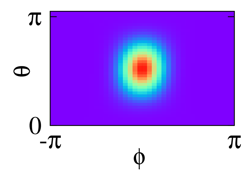
(b)

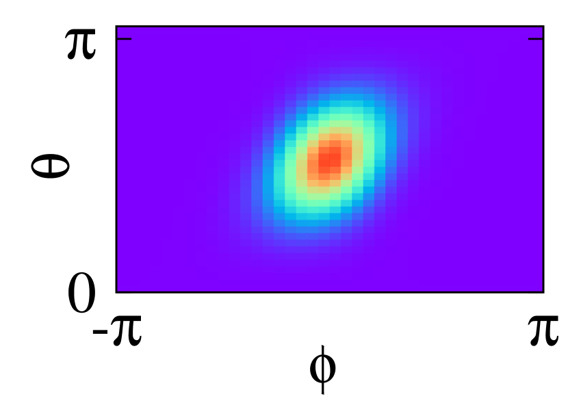
(c)

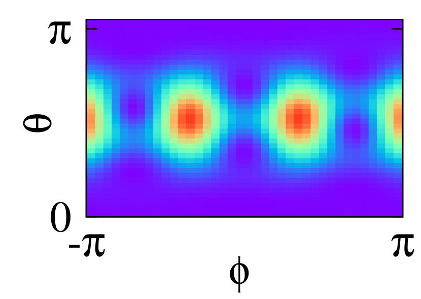
(d)

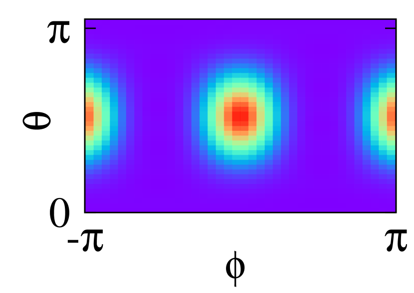
Figure 1: (Color online) Husimi functions in the absence of losses in the BJJ at some specific times: (a) $t=0$ (coherent state); (b) $t=T/40$ (spin squeezed state) , (c) $t=T/6$ (3-component superposition of phase states), (d) $t=T/4$ (2-component superposition). Other parameters: $U_{1}=U_{2}=\frac{2\pi}{T}$, $U_{12}=0$, $E_{1}=E_{2}=0$, and $N_{0}=10$.

II.1.3 Master equation in the presence of atom losses

We account for loss processes in the BJJ by considering the Markovian master equation anglin1997 ; jack2002 ; jack2003

$$\frac{{\rm{d}}\hat{\rho}}{{\rm{d}}t}=-{\rm{i}}\bigl{[}\hat{H}_{0},\hat{\rho}(t)\bigr{]}+({{\cal L}}_{\text{1-body}}+{{\cal L}}_{\text{2-body}}+{{\cal L}}_{\text{3-body}})(\hat{\rho}(t))$$ (14)

where we have set $\hbar=1$, $\hat{\rho}(t)$ is the atomic density matrix, and the superoperators ${{\cal L}}_{\text{1-body}}$, ${{\cal L}}_{\text{2-body}}$, and ${{\cal L}}_{\text{3-body}}$ describe one-body, two-body, and three-body losses, respectively. They are given by

$${{\cal L}}_{\text{1-body}}(\hat{\rho}) = \sum_{i=1,2}\alpha_{i}\Bigl{(}\hat{a}_{i}\,\hat{\rho}\,{\hat{a}_{i}}^{\dagger}-\frac{1}{2}\bigl{\{}\hat{n}_{i},\hat{\rho}\bigr{\}}\Bigr{)}$$

$${{\cal L}}_{\text{2-body}}(\hat{\rho}) = \sum_{1\leq i\leq j\leq 2}\gamma_{ij}\Bigl{(}\hat{a}_{i}\hat{a}_{j}\,\hat{\rho}\,{\hat{a}_{i}}^{\dagger}\hat{a}_{j}^{\dagger}-\frac{1}{2}\bigl{\{}{\hat{a}_{i}}^{\dagger}\hat{a}_{j}^{\dagger}\hat{a}_{i}\hat{a}_{j},\hat{\rho}\bigr{\}}\Bigr{)}$$

$${{\cal L}}_{\text{3-body}}(\hat{\rho}) = \sum_{1\leq i\leq j\leq k\leq 2}\kappa_{ijk}\Bigl{(}\hat{a}_{i}\hat{a}_{j}\hat{a}_{k}\,\hat{\rho}\,\hat{a}_{i}^{\dagger}\hat{a}_{j}^{\dagger}\hat{a}_{k}^{\dagger}$$ (15)

$$\hskip 14.22636pt-\frac{1}{2}\bigl{\{}\hat{a}_{i}^{\dagger}\hat{a}_{j}^{\dagger}\hat{a}_{k}^{\dagger}\hat{a}_{i}\hat{a}_{j}\hat{a}_{k},\hat{\rho}\bigr{\}}\Bigr{)}\;,$$

where the rates $\alpha_{i}$, $\gamma_{ij}$, and $\kappa_{ijk}$ correspond to the loss of one atom in the mode $i$, of two atoms in the modes $i$ and $j$, and of three atoms in the modes $i$, $j$, and $k$ (with $i,j,k=1,2$), respectively, and $\{\cdot,\cdot\}$ denotes the anti-commutator. To shorten notation we write the loss rate of two (three) atoms in the same mode $i$ as $\gamma_{i}=\gamma_{ii}$ ($\kappa_{i}=\kappa_{iii}$) and set $\kappa_{12}=\kappa_{112}$ and $\kappa_{21}=\kappa_{122}$. Note that the inter-mode rates $\gamma_{12}$, $\kappa_{12}$, and $\kappa_{21}$ vanish for external BJJs. The loss rates depend on the macroscopic wave function of the condensate and thus on the number of atoms and interaction energies $U_{i}$. As far as the number of lost atoms at the revival time $T$ remains small with respect to the initial atom number $N_{0}$, one may, however, assume that these rates are time-independent in the time interval $[0,T]$. Hereafter we always assume that this is the case.

II.1.4 Conditional states

The master equation (14) does not couple sectors with different numbers of atoms $N$. As a result, if the density matrix $\hat{\rho}(t)$ has initially no coherences between states with different $N$’s then such coherences are absent at all times $t\geq 0$. Hence

$$\hat{\rho}(t)=\sum_{N=0}^{N_{0}}\widetilde{\rho}_{N}(t)\quad,\quad\widetilde{\rho}_{N}(t)=w_{N}(t)\hat{\rho}_{N}(t)\;,$$ (16)

where $\widetilde{\rho}_{N}(t)$ ($\hat{\rho}_{N}(t)$) is the unnormalized (normalized) density matrix with a well-defined atom number $N$ (that is, $\langle n_{1},n_{2}|\widetilde{\rho}_{N}(t)|n_{1}^{\prime},n_{2}^{\prime}\rangle=0$ for $n_{1}+n_{2}\not=N$ or $n_{1}^{\prime}+n_{2}^{\prime}\not=N$) and $w_{N}(t)\geq 0$ is the probability of finding $N$ atoms in the BJJ at time $t$ (thus $\sum_{N}w_{N}(t)=1$). The matrix $\hat{\rho}_{N}(t)$ is the conditional state following a measurement of $\hat{N}$. More precisely, it describes the state of the BJJ when one selects among many single-run experiments those for which the measured atom number at time $t$ is equal to $N$ and one averages all experimental results over these “post-selected” single-run experiments, disregarding all the others. In this sense, $\hat{\rho}_{N}(t)$ contains a more precise physical information than the total density matrix $\hat{\rho}(t)$. To have access to this information, one must be able to extract samples with a well-defined number of atoms initially (since we assumed an initial state with $N_{0}$ atoms) and after the evolution time $t$. Even though the precise measurement of $\hat{N}$ is still an experimental challenge, the precision has increased by orders of magnitude during the last years itah2010 ; gross2011 ; hume2013 .

II.2 Quantum correlations useful for interferometry

A useful quantity characterizing quantum correlations (QCs) between particles in systems involving many atoms is the quantum Fisher information. Let us recall briefly its definition and its link with phase estimation in atom interferometry (see Klauder1986 ; ferrini2010 ; pezze09 for more detail). In a Mach-Zehnder atom interferometer, an input state $\hat{\rho}_{\text{in}}$ is first transformed into a superposition of two modes, analogous to the two arms of an optical interferometer. These modes acquire distinct phases $\varphi_{1}$ and $\varphi_{2}$ during the subsequent quantum evolution and are finally recombined to read out interference fringes, from which the phase shift $\varphi=\varphi_{1}-\varphi_{2}$ is inferred. We assume in the whole paper that during this interferometric sequence one can neglect inter-particle interactions (nonlinear terms in the Hamiltonian (6)) and loss processes. This is well justified in the experiments of Ref. gross2010 . The dependence of the phase sensitivity on inter-particle interactions has been studied in Grond11 ; tikhonenkov10 . Under this assumption, the output state of the interferometer is $\hat{\rho}_{\text{out}}(\varphi)=e^{-{\rm{i}}\varphi\hat{J}_{\vec{n}}}\hat{\rho}_{\text{in}}e^{{\rm{i}}\varphi\hat{J}_{\vec{n}}}$, where $\hat{J}_{\vec{n}}=n_{x}\hat{J}_{x}+n_{y}\hat{J}_{y}+n_{z}\hat{J}_{z}$ is the angular momentum generating a rotation on the Bloch sphere along the axis defined by the unit vector $\vec{n}$, with $\hat{J}_{x}=(\hat{a}^{\dagger}_{1}\hat{a}_{2}+\hat{a}^{\dagger}_{2}\hat{a}_{1})/2$, $\hat{J}_{y}=-i(\hat{a}^{\dagger}_{1}\hat{a}_{2}-\hat{a}^{\dagger}_{2}\hat{a}_{1})/2$, and $\hat{J}_{z}=(\hat{a}^{\dagger}_{1}\hat{a}_{1}-\hat{a}^{\dagger}_{2}\hat{a}_{2})/2$.

The phase shift $\varphi$ is determined by means of a statistical estimator depending on the results of measurements on the output state $\hat{\rho}_{\text{out}}(\varphi)$. The best precision on $\varphi$ that can be achieved (that is, optimizing over all possible estimators and measurements) is given by braunstein1994

$$(\Delta\varphi)_{\text{best}}=\frac{1}{\sqrt{{\cal{M}}\,F(\hat{\rho}_{\rm in},\hat{J}_{\vec{n}})}}\;,$$ (17)

where ${\cal{M}}$ is the number of measurements and

$$F(\hat{\rho},\hat{J}_{\vec{n}})=2\sum_{k,l,p_{k}+p_{l}>0}\frac{(p_{k}-p_{l})^{2}}{p_{k}+p_{l}}\bigl{|}\langle k|\hat{J}_{\vec{n}}|l\rangle\bigr{|}^{2}$$ (18)

is the quantum Fisher information. Here, $\{|l\rangle\}$ is an orthonormal basis diagonalizing $\hat{\rho}$, $\hat{\rho}|l\rangle=p_{l}|l\rangle$. The quantum Fisher information thus measures the amount of QCs in the input state that can be used to enhance phase sensitivity with respect to the shot noise limit $(\Delta\varphi)_{\rm SN}=1/\sqrt{{\cal{M}}\,\langle\hat{N}\rangle}$, that is, to the sensitivity obtained by using $\langle\hat{N}\rangle$ independent atoms. Since $\hat{J}_{\vec{n}}$ does not couple subspaces with different $N$’s, it follows from Eq.(18) and from the block structure (16) of $\hat{\rho}$ that

$$F(\hat{\rho},\hat{J}_{\vec{n}})=\sum_{N=0}^{N_{0}}w_{N}F(\hat{\rho}_{N},\hat{J}_{\vec{n}})\;,$$ (19)

where $F_{N}(\hat{\rho}_{N},\hat{J}_{\vec{n}})$ is the Fisher information of the conditional state $\hat{\rho}_{N}$ with $N$ atoms and $w_{N}$ is the corresponding probability.

It is shown in HyllusPRL2010 that if $F(\hat{\rho},\hat{J}_{\vec{n}})$ is larger than the average number of atoms $\langle\hat{N}\rangle$ then the atoms are entangled. According to Eq.(17), the condition $F(\hat{\rho},\hat{J}_{\vec{n}})>\langle\hat{N}\rangle$ is a necessary and sufficient condition for sub-shot noise sensitivity $(\Delta\varphi)_{\text{best}}<(\Delta\varphi)_{\rm SN}$.

In order to obtain a measure of QCs independent of the direction $\vec{n}$ of the interferometer, we optimize the Fisher information over all unit vectors $\vec{n}$ and define Hyllus2010 ,

$$F(\hat{\rho})=\max_{\|\vec{n}\|=1}F(\hat{\rho},\hat{J}_{\vec{n}})=4C_{\rm max}\;.$$ (20)

Here, $C_{\rm max}$ is the largest eigenvalue of the $3\times 3$ real symmetric covariance matrix

$$C_{ab}=\frac{1}{2}\sum_{k,l,p_{k}+p_{l}>0}\frac{(p_{k}-p_{l})^{2}}{p_{k}+p_{l}}\mathrm{Re}\,\bigl{\{}\langle k|\hat{J}_{a}|l\rangle\langle l|\hat{J}_{b}|k\rangle\bigr{\}}\;,$$ (21)

with $a,b=1,2,3$. For simplicity we write $F_{\rm tot}(t)\equiv F(\hat{\rho}(t))$ for the optimized Fisher information of the total atomic density matrix $\hat{\rho}(t)$ at time $t$ (note that the direction $\vec{n}$ maximizing $F(\hat{\rho},\hat{J}_{\vec{n}})$ depends on $t$). When studying the QCs in the conditional states we optimize over $\vec{n}$ independently in each subspace and define $F_{N}(t)$ as in (20), by replacing $\hat{\rho}$ by $\hat{\rho}_{N}(t)$ in this formula. Note that $F_{\rm tot}(t)$ is not equal to $\sum_{N}w_{N}(t)F_{N}(t)$, because the optimal directions may be different in each subspace.

In the absence of losses, the two-component superposition of CSs has the highest possible Fisher information $F[\hat{\rho}^{(0)}(t_{2})]=N_{0}^{2}$, which is for $N_{0}\gg 1$ approximately twice larger than that of the superpositions with $q$ components, $3\leq q\lesssim N_{0}^{1/2}$ pezze09 ; ferrini2010 . The upper solid curve in Fig. 2(a) shows $F_{\rm tot}(t)$ in the absence of losses as a function of time for $N_{0}=10$ atoms in the BJJ.

(a) symmetric case

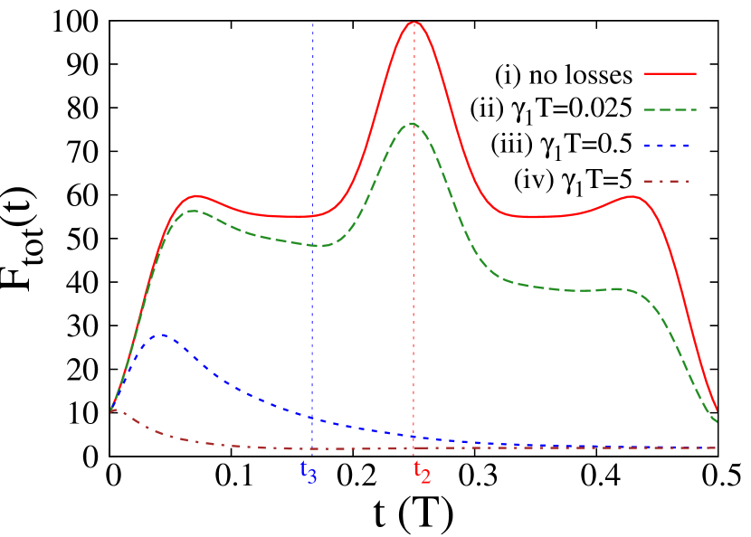
(b) $\gamma_{1}T=\gamma_{2}T=0.5$

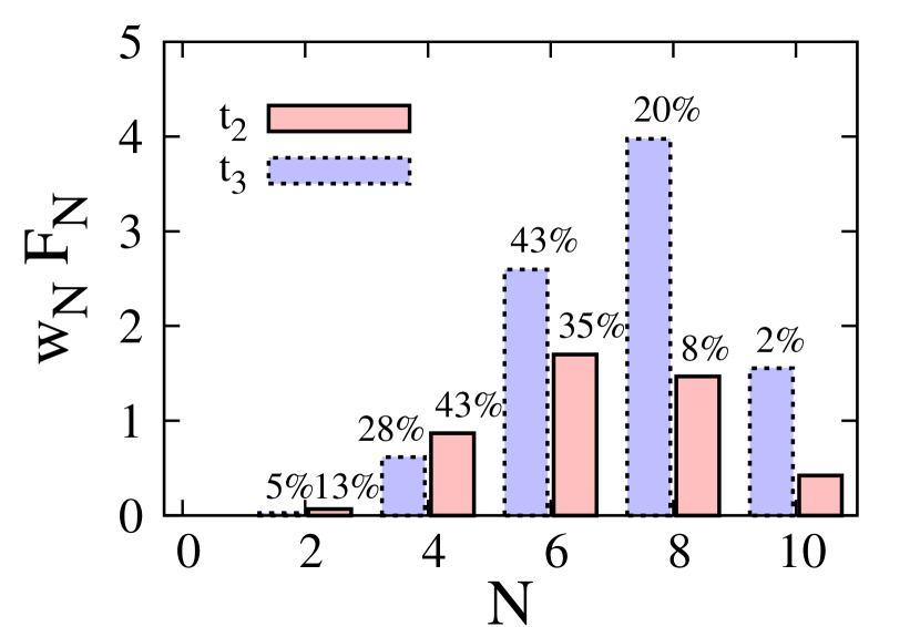
(c) all cases

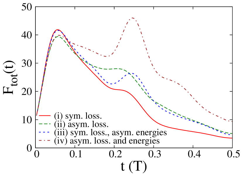
(d) $t=t_{2}=T/4$

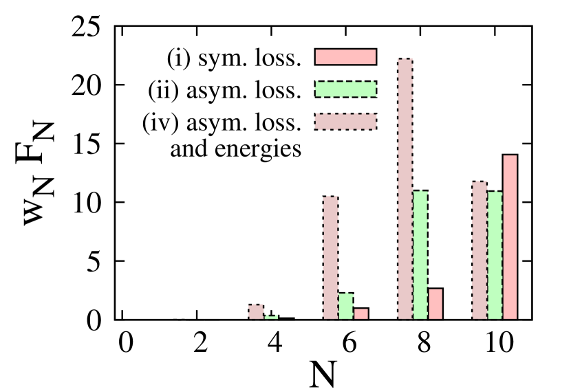
Figure 2: (Color online) (a) Total quantum Fisher information $F_{\rm tot}(t)$ versus time $t$ (in units of $T=2\pi/\chi$) for symmetric two-body loss rates $\gamma_{1}=\gamma_{2}$ in each mode and $\gamma_{12}=\alpha_{i}=\kappa_{i}=\kappa_{ij}=0$. The different curves correspond to (from top to bottom) $\gamma_{1}T=0$, $0.025$, $0.5$, and $5$. The dotted vertical lines indicate the formation times $t_{2}=T/4$ and $t_{3}=T/6$ of the 2- and 3-component superpositions. The histogram (b) shows the contributions $w_{N}F_{N}(\hat{\rho}_{N},J_{\vec{n}_{\text{opt}}})$ to $F_{\rm tot}$ of the subspaces with different atom numbers $N$ [see Eq.(19)] for two different times, $t_{2}$ (pink boxes) and $t_{3}$ (blue boxes), and for the loss rates indicated above the histogram. The percentages on top of each boxes are the probabilities $w_{N}$ of finding $N$ atoms at these times (weights smaller than 1% are not indicated). (c) Same as in (a) for (i) symmetric losses ($\gamma_{1}=\gamma_{2}=0.177/T$) and energies ($U_{1}=U_{2}$); (ii) asymmetric losses ($\gamma_{1}=0.6/T$, $\gamma_{2}=0$) and symmetric energies ($U_{1}=U_{2}$); (iii) symmetric losses ($\gamma_{1}=\gamma_{2}=0.177/T$) and asymmetric energies ($U_{2}=U_{12}<U_{1}$); (iv) asymmetric losses ($\gamma_{1}=0$, $\gamma_{2}=0.6/T$) and energies ($U_{2}=U_{12}<U_{1}$). The loss rates are chosen in such a way that the number of lost atoms at time $t_{2}$ is the same and equal to about 3 in all cases. The interaction energies $U_{i}$ are such that $T=4\pi/(U_{1}+U_{2}-2U_{12})$ is the same in all cases. (d) Histogram of the contributions of the subspaces with $N$ atoms to $F_{\rm tot}(t_{2})$ for the same values of $\gamma_{i}$ and $U_{i}$ as in (c) in the cases (i) (right pink boxes), (ii) (middle green boxes), and (iv) (left purple boxes). In all panels $N_{0}=10$, $\gamma_{12}=0$, and one- and three-body losses are absent. All results are obtained from the exact diagonalization method (see Appendix A).

II.3 Quantum trajectories

We solve the master equation (14) using two methods: the quantum jump approach and an exact diagonalization. We outline in this section the first approach, which yields a tractable analytical solution in the case of few loss events and gives physical intuition on the various decoherence mechanisms. This approach will be used to explain the results provided by the exact diagonalization method, which offers the exact solution for the whole density matrix when inter-mode losses are absent, i.e. $\gamma_{12}=\kappa_{21}=\kappa_{12}=0$. The exact diagonalization method is described in Appendix A. We use it mostly to compute numerically the Fisher information.

In the quantum jump description, the state of the atoms is a pure state $|\psi(t)\rangle$ which evolves randomly in time as follows carmichael1991 ; moelmer1993 ; belavkin1990 ; barchielli1991 ; Knight98 ; Haroche . At random times $s$ quantum jumps occur and the atomic state is transformed as

$$|\psi(s-)\rangle\longrightarrow|\psi(s+)\rangle=\frac{\hat{M}_{m}|\psi(s-)\rangle}{\|\hat{M}_{m}|\psi(s-)\rangle\|}\;,$$ (22)

where the index $m$ labels the type of jump and $\hat{M}_{m}$ is the corresponding jump operator. In our case, restricting for the moment our attention to two-body losses, one has three types of jumps: the loss of two atoms in the first mode, with $\hat{M}_{2,0}=\hat{a}_{1}^{2}$, the loss of two atoms in the second mode, with $\hat{M}_{0,2}=\hat{a}_{2}^{2}$, and the loss of one atom in each mode, with $\hat{M}_{1,1}=\hat{a}_{1}\hat{a}_{2}$. The probability that a jump $m$ occurs in the infinitesimal time interval $[s,s+{\rm{d}}s]$ is ${\rm{d}}p_{m}(s)=\Gamma_{m}\|\hat{M}_{m}|\psi(s)\rangle\|^{2}{\rm{d}}s$, where $\Gamma_{m}$ is the jump rate in the loss channel $m$. Using the notation of Sec. II.1.3, one has $\Gamma_{2,0}=\gamma_{1}$, $\Gamma_{0,2}=\gamma_{2}$, and $\Gamma_{1,1}=\gamma_{12}$. Between jumps, the wave function $|\psi(t)\rangle$ evolves according to the effective non self-adjoint Hamiltonian $\hat{H}_{\rm eff}=\hat{H_{0}}-{\rm{i}}\hat{D}_{\rm 2-body}$ with

$$\hat{D}_{\rm 2-body} = \frac{1}{2}\sum_{m}\Gamma_{m}\hat{M}_{m}^{\dagger}\hat{M}_{m}$$

$$= \frac{1}{2}\sum_{i=1,2}\gamma_{i}\hat{n}_{i}(\hat{n}_{i}-1)+\frac{\gamma_{12}}{2}\hat{n}_{1}\hat{n}_{2}\,.$$

The physical origin of the damping term comes from the gain of information acquired on the atomic state by conditioning the system to have no loss in a given time interval moelmer1993 ; Haroche : the longer the time interval, the smaller must be the number of atoms left in the BJJ in the mode losing atoms.

The random wave function at time $t$ reads

$$|\psi_{J}(t)\rangle = \frac{|\widetilde{\psi}_{J}(t)\rangle}{\|{\widetilde{\psi}_{J}(t)}\|}$$

$$|\widetilde{\psi}_{J}(t)\rangle = e^{-{\rm{i}}(t-s_{J})\hat{H}_{\rm eff}}\hat{M}_{m_{J}}e^{-{\rm{i}}(s_{J}-s_{J-1})\hat{H}_{\rm eff}}\hat{M}_{m_{J-1}}\cdots$$ (24)

$$\cdots e^{-{\rm{i}}\hat{H}_{\rm eff}(s_{2}-s_{1})}\hat{M}_{m_{1}}e^{-{\rm{i}}s_{1}\hat{H}_{\rm eff}}|\psi(0)\rangle\;,$$

where $J$ is the number of loss events in the time interval $[0,t]$, $0\leq s_{1}\leq\cdots\leq s_{J}\leq t$ are the random loss times, and $m_{1},\ldots,m_{J}$ the random loss types. The time evolution of the wave function $t\mapsto|\psi_{J}(t)\rangle$ for a fixed realization of the jump process is called a quantum trajectory.

The probability to have no atom loss between times $0$ and $t$ is given by $\|e^{-{\rm{i}}t\hat{H}_{\rm eff}}|\psi(0)\rangle\|^{2}$. The probability to have $J$ loss events in $[0,t]$, with the $\nu$th event of type $m_{\nu}$ occurring in the time interval $[s_{\nu},s_{\nu}+{\rm{d}}s_{\nu}]$, $\nu=1,\ldots,J$, is

$${\rm{d}}p_{m_{1},\ldots,m_{J}}^{(t)}(s_{1},\ldots,s_{J};J)$$

$$\hskip 28.45274pt=\Gamma_{m_{1}}\ldots\Gamma_{m_{J}}\|{\widetilde{\psi}_{J}(t)}\|^{2}{\rm{d}}s_{1}\ldots{\rm{d}}s_{J}\,.$$ (25)

The link of this approach with the master equation description is that the average over all quantum trajectories (that is, over the number of jumps $J$, the jump times $s_{\nu}$, and the jump types $m_{\nu}$) of the rank-one projector $|\psi_{J}(t)\rangle\langle\psi_{J}(t)|$ yields the density matrix $\hat{\rho}(t)$ solution of the master equation (14) moelmer1993 . We thus recover the block structure (16) of the atomic density matrix, with

$$\widetilde{\rho}_{N_{J}}(t) = \sum_{m_{1},\ldots,m_{J}}\Gamma_{m_{1}}\ldots\Gamma_{m_{J}}\int_{0\leq s_{1}\leq\cdots\leq s_{J}\leq t}{\rm{d}}s_{1}\ldots{\rm{d}}s_{J}$$ (26)

$$|\widetilde{\psi}_{J}(t)\rangle\langle\widetilde{\psi}_{J}(t)|\;,$$

where we have set $N_{J}=N_{0}-2J$. Therefore, quantum trajectories provide a natural and efficient tool to study the conditional states $\hat{\rho}_{N_{J}}(t)$ with $N_{J}$ atoms, which only depend on quantum trajectories having $J$ two-body loss events.

It is straightforward to extend the above description to include also one- and three-body losses. This is achieved by adding new types of jumps with jump operators $\hat{M}_{1,0}=\hat{a}_{1}$, $\hat{M}_{0,1}=\hat{a}_{2}$ (for one-body losses) and $\hat{M}_{3,0}=\hat{a}_{1}^{3}$, $\hat{M}_{0,3}=\hat{a}_{2}^{3}$, $\hat{M}_{2,1}=\hat{a}_{1}^{2}\hat{a}_{2}$, and $\hat{M}_{1,2}=\hat{a}_{1}\hat{a}_{2}^{2}$ (for three-body losses). The corresponding jump rates are $\Gamma_{1,0}=\alpha_{1}$, $\Gamma_{0,1}=\alpha_{2}$, $\Gamma_{3,0}=\kappa_{1}$, $\Gamma_{0,3}=\kappa_{2}$, $\Gamma_{2,1}=\kappa_{12}$, and $\Gamma_{1,2}=\kappa_{21}$. The conditional state $\hat{\rho}_{N}(t)$ is obtained by summing the right-hand side of Eq.(26) over all $J$ and all $r_{1},\ldots,r_{J}\in\{1,2,3\}$ such that $N_{0}-\sum_{\nu=1}^{J}r_{\nu}=N$, $r_{\nu}$ being the number of atoms lost in the $\nu$th loss event. The effective Hamiltonian becomes $\hat{H}_{\rm eff}=\hat{H}_{0}-{\rm{i}}\hat{D}$ with $\hat{D}=\hat{D}_{\rm 1-body}+\hat{D}_{\rm 2-body}+\hat{D}_{\rm 3-body}$ and

$$\hat{D}_{\rm 1-body} = \frac{1}{2}\sum_{i=1,2}\alpha_{i}\hat{n}_{i}$$ (27)

$$\hat{D}_{\rm 3-body} = \frac{1}{2}\sum_{i=1,2}\kappa_{i}\hat{n}_{i}(\hat{n}_{i}-1)(\hat{n}_{i}-2)$$ (28)

$$+\frac{1}{2}\sum_{i\not=j}\kappa_{ij}\hat{n}_{i}(\hat{n}_{i}-1)\hat{n}_{j}\,.$$

III Main results

We present in this section our main results on the time evolution of the QCs in the atomic state under the quenched dynamics in the presence of atom losses. The amount of QCs is estimated by the total quantum Fisher information $F_{\rm tot}(t)$.

Before investigating the combined effect of the various loss processes, we start by a detailed analysis of a small atomic sample with $N_{0}=10$ atoms subject to two-body losses only and without inter-mode losses (the latter losses cannot be addressed by our exact diagonalization and will be discussed in Sec. IV). Figure 2 shows the effect of increasing the loss rates in a symmetric model with $\gamma_{1}=\gamma_{2}$ and $U_{1}=U_{2}$ (panel (a)). The Fisher information, which in the absence of losses is characterized by a broad peak at the time $t_{2}=T/4$ of formation of the two-component superposition, rapidly decreases once the loss rate increases. If, however, an asymmetric model is chosen – with parameters yielding the same average number of lost atoms at time $t_{2}$ and the same revival time $T$ as in the symmetric case – we find that the Fisher information is considerably increased (panel (c) in Fig. 2). The most favorable situation turns out to be the one with asymmetric energies $U_{2}=U_{12}<U_{1}$ and vanishing loss rate $\gamma_{1}=0$ in the mode with largest interactions (a similar result would be obtained for $U_{1}=U_{12}<U_{2}$ and $\gamma_{2}=0$). The histograms shown in panels (b) and (d) in Fig. 2 give the contributions $w_{N}(t)F(\hat{\rho}_{N}(t),\hat{J}_{\vec{n}})$ to $F_{\rm tot}(t)$ of the various subspaces with fixed atom numbers $N$ (see (19)), evaluated in the direction $\vec{n}=\vec{n}_{\rm opt}$ optimizing the Fisher information of the total state, for $t=t_{2},t_{3}$. One infers from these histograms that the aforementioned effect is non-trivial, namely, the large Fisher informations at times $t_{2}$ and $t_{3}$ for asymmetric rates and energies do not come from the contribution of the subspace with $N=N_{0}$.

We study now an atomic sample with $N_{0}=100$ atoms initially in the case where several loss processes are combined together. Figure 3 shows the total quantum Fisher information for experimentally relevant parameters extracted from Refs. sinatra1998 ; riedel2010 ; yun2009 (we explain how these parameters are obtained in Appendix B). As can be seen in this figure, in the presence of two-body asymmetric losses only, the QCs of the superpositions are well preserved as in the small atomic sample discussed above. This asymmetric situation is realized in the experiment of Ref. gross2010 , the two-body losses occurring mainly in the upper internal level gross2010dissJPB . When one- and three-body losses – which are also present in this experiment – are added, the coherences of the superpositions are still preserved provided that all losses occur in the second mode (upper energy level). In this case, the QCs can be protected against atom losses by tuning the interaction energy $U_{2}$ such that $U_{2}=U_{12}$. This shows that the results of Ref. pawlowski2013 concerning two-body losses hold for one- and three-body losses as well. However, when symmetric one-body or three-body losses are added, the QCs are destroyed on a much shorter time scale and the peak in the Fisher information at time $t_{2}$ disappears. In the experiments of Refs. riedel2010 ; gross2010 , the one-body losses are symmetric since they are due to collisions with atoms from the background gas, which are equally likely for the two internal atomic states. These one-body symmetric losses are therefore much more detrimental to the QCs than asymmetric two-body losses.

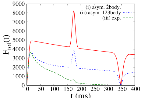
Figure 3: (Color online) Total quantum Fisher information $F_{\rm tot}(t)$ versus time $t$ (in units of $T$) from exact diagonalization for more realistic experimental conditions (see Appendix B) with $N_{0}=100$, $U_{2}=U_{12}$, $U_{1}-U_{12}=18.056$Hz, and (i) asymmetric two-body losses $\gamma_{2}=0.0127$Hz and $\gamma_{1}=0$ without one- and three-body losses; (ii) one-, two-, and three-body losses in the second mode with rates $\alpha_{2}=0.4$Hz, $\gamma_{2}=0.0127$Hz, $\kappa_{2}=1.08\times 10^{-6}$Hz, and no losses in the first mode; (iii) symmetric one- and three-body losses and asymmetric two-body losses, $\alpha_{1}=\alpha_{2}=0.2$Hz, $\gamma_{2}=0.0127$Hz, $\gamma_{1}=0$, and $\kappa_{1}=\kappa_{2}=0.54\times 10^{-6}$Hz. The case (iii) roughly corresponds to the experimental conditions in Refs. riedel2010 ; gross2010 .

IV Quantum correlations in the subspaces with fixed atom numbers

IV.1 Overview of the results from the quantum jump method

In order to explain the behavior of the total Fisher information observed in the exact diagonalization approach, we analyze separately the contributions of each subspace with a fixed atom number to the total Fisher information. This is done by using the quantum jump approach of Sec. II.3. We argue in what follows that the stronger decoherence for symmetric two-body loss rates and energies in Fig. 2(c) originates from a “destructive interference” (exact cancellation) when adding the contributions of the two loss channels at time $t_{2}$. A similar cancellation occurs at time $t_{3}$ for symmetric three-body losses, but it is absent for one-body losses. Moreover, the weaker decoherence for completely asymmetric losses obtained by tuning the interaction energies as described above comes from the absence of dephasing in the mode $i$ losing atoms. This effect is somehow trivial for external BJJs: there this absence of dephasing occurs for a vanishing interaction energy $U_{i}=U_{12}=0$; for such $U_{i}$ the collision processes responsible of two-body losses in the mode $i$ are suppressed (moreover, our assumption that the loss rates are independent of the energies is not justified anymore). In contrast, for internal BJJs decoherence is reduced when $U_{i}$ is equal to the inter-mode interaction $U_{12}\not=0$ and the effect is non-trivial. We shall explain it by invoking the effective phase noise produced by atom losses in the presence of interactions sinatra2012 ; pawlowski2013 .

IV.2 Conditional state in the subspace with the initial number of atoms

$\quad\gamma_{1}T=0$

$\quad\gamma_{1}T=2$

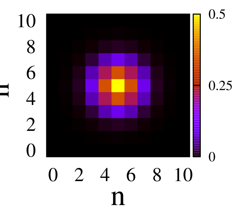
$\quad\gamma_{1}T=10$

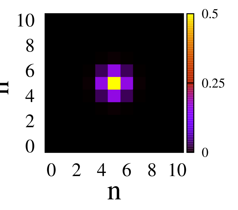
$\quad\gamma_{1}T=20$

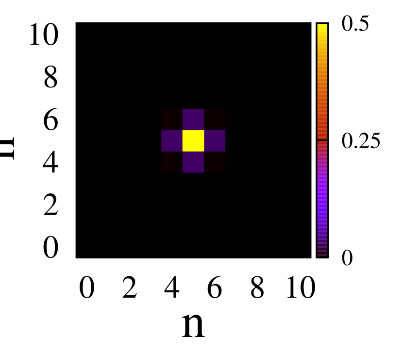
$\gamma_{1}T=0$

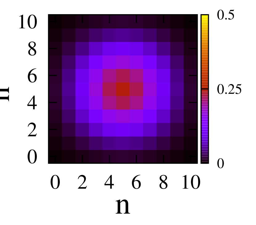
$\gamma_{1}T=4$

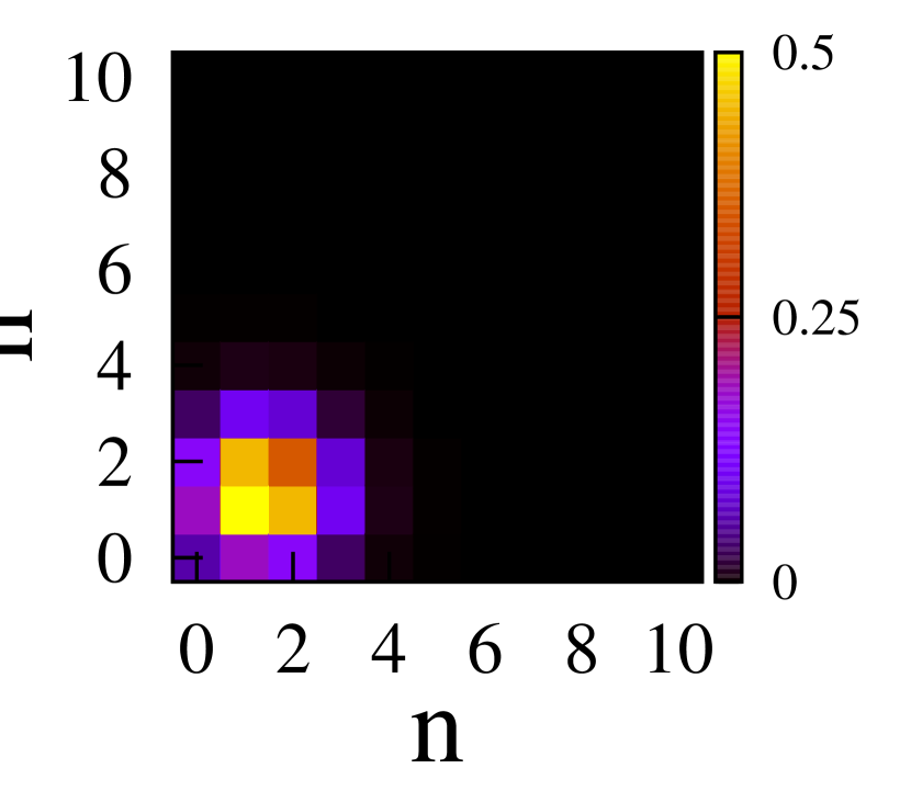
$\gamma_{1}T=20$

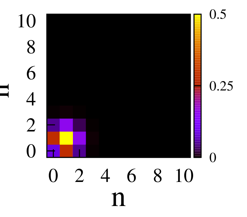
$\gamma_{1}T=40$

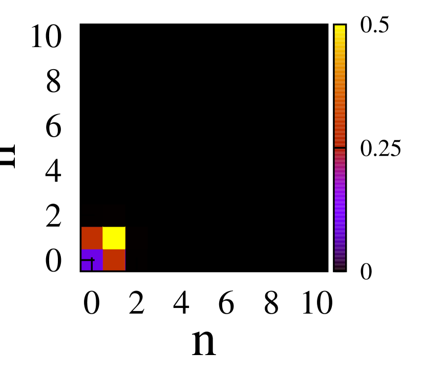
Figure 4: (Color online) Moduli of the matrix elements in the Fock basis of the state $\hat{\rho}_{N_{0}}(t_{3})$ in the subspace with $N_{0}$ atoms at the time of formation $t_{3}=T/6$ of the 3-component superposition, from the exact diagonalization method. Upper panels: symmetric two-body losses ($\gamma_{1}=\gamma_{2}$). Lower panels: completely asymmetric two-body losses ($\gamma_{2}=0$). The values of $\gamma_{1}$ are indicated on the top of each panel. Other parameters: $\alpha_{i}=\gamma_{12}=\kappa_{i}=\kappa_{ij}=0$ and $N_{0}=10$.

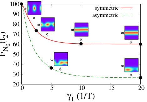
Figure 5: (Color online) Fisher information $F_{N_{0}}(t_{2})$ optimized in the subspace with $N_{0}$ atoms at time $t_{2}$ as a function of the loss rate $\gamma_{1}$ (in units of $T^{-1}$). Solid line: symmetric losses ($\gamma_{1}=\gamma_{2}$). Dashed line: asymmetric losses ($\gamma_{2}=0$). The Husimi functions are plotted in the insets for some specific choices of loss rates indicated by circles on the two curves. Other parameters as in Fig. 4.

We start by determining the conditional state $\hat{\rho}_{N_{0}}(t)$ with the initial number of atoms $N_{0}$ at time $t$. In the quantum jump approach this corresponds to the contribution of quantum trajectories with no jump in the time interval $[0,t]$, which are given by (see Sec. II.3)

$$|\widetilde{\psi}_{0}(t)\rangle=e^{-{\rm{i}}t(\hat{H}_{0}-{\rm{i}}\hat{D})}|N_{0};\phi=0\rangle\,.$$ (29)

The unnormalized conditional state is $\widetilde{\rho}_{N_{0}}^{\rm{(no\,loss)}}(t)=|\widetilde{\psi}_{0}(t)\rangle\langle\widetilde{\psi}_{0}(t)|$. In the Fock basis diagonalizing both $\hat{H}_{0}$ and $\hat{D}$, it takes the form

$$\langle n_{1},n_{2}|\widetilde{\rho}_{N_{0}}^{\rm{(no\,loss)}}(t)|n_{1}^{\prime},n_{2}^{\prime}\rangle=$$

$$\hskip 17.07182pte^{-t[d_{N_{0}}(n_{1})+d_{N_{0}}(n_{1}^{\prime})]}\langle n_{1},n_{2}|\hat{\rho}^{(0)}_{N_{0}}(t)|n_{1}^{\prime},n_{2}^{\prime}\rangle\;,$$ (30)

where $\hat{\rho}^{(0)}_{N_{0}}(t)$ is the state in the absence of losses (see Sec. II.1.2), $n_{2}=N_{0}-n_{1}$, $n_{2}^{\prime}=N_{0}-n_{1}^{\prime}$, and $d_{N_{0}}(n_{1})=\langle n_{1},n_{2}|\hat{D}|n_{1},n_{2}\rangle$. The probability to find $N_{0}$ atoms at time $t$ is found with the help of Eqs.(10) and (IV.2). One finds

$$w_{N_{0}}(t)=\operatorname{tr}\widetilde{\rho}_{N_{0}}^{\rm{(no\,loss)}}(t)=\frac{1}{2^{N_{0}}}\sum_{n_{1}=0}^{N_{0}}\left(\begin{array}[]{c}N_{0}\\ n_{1}\end{array}\right)e^{-2td_{N_{0}}(n_{1})}\,.$$ (31)

In the following we restrict our attention to symmetric three-body losses $\kappa_{1}=\kappa_{2}$ and $\kappa_{12}=\kappa_{21}$. The asymmetric three-body loss case is treated in Appendix C. Let us set $\kappa=(3\kappa_{1}-\kappa_{12})/2$ and

$$a=\frac{1}{2}\bigl{(}\gamma_{1}+\gamma_{2}-\gamma_{12}\bigr{)}+(N_{0}-2)\kappa\,.$$ (32)

If $a\not=0$, the damping factor in Eq.(IV.2) (i.e. the exponential factor in the right-hand side) is Gaussian. Actually, by using Eqs.(II.3), (27), and (28), one obtains

$$d_{N_{0}}(n_{1})=a(n_{1}-\overline{n}_{1})^{2}+c\;,$$ (33)

where $c$ is an irrelevant $n_{1}$-independent constant which can be absorbed in the normalization of the density matrix, and

$$\overline{n}_{1}=\frac{1}{4a}\Bigl{(}\Delta\alpha-\Delta\gamma+N_{0}(2\gamma_{2}-\gamma_{12})+2N_{0}(N_{0}-2)\kappa\Bigr{)}$$ (34)

with $\Delta\alpha=\alpha_{2}-\alpha_{1}$ and $\Delta\gamma=\gamma_{2}-\gamma_{1}$.

In order to estimate the QCs in $\hat{\rho}_{N_{0}}(t)$ and the typical loss rates at which this state is affected by the Gaussian damping, we now focus on three particular cases.

(i) Symmetric loss rates $\gamma_{1}=\gamma_{2}$ and $\alpha_{1}=\alpha_{2}$. In this case $a=\gamma/2+(N_{0}-2)\kappa$ with $\gamma=2\gamma_{1}-\gamma_{12}$ and $\overline{n}_{1}=N_{0}/2$. Hence the damping factor in Eq.(IV.2) is a Gaussian centered at $(n_{1},n_{1}^{\prime})=(N_{0}/2,N_{0}/2)$. This center coincides with the peak of the matrix elements in the absence of losses, which have a width $\approx\sqrt{N_{0}}$, see Eq.(11). Thus the effect of the Gaussian damping begins to set in for times $t$ such that $at\approx 1/N_{0}$. In particular, the macroscopic superposition at time $t_{q}=\pi/(\chi q)$ is noticeably affected by damping for $a\gtrsim\chi q/N_{0}$. It is shown in Appendix C that $\hat{\rho}_{N_{0}}(t_{q})$ converges at large loss rates $a\gg\chi q$ to the pure Fock state $|N_{0}/2,N_{0}/2\rangle$ with equal numbers of atoms in each mode if $N_{0}$ is even, as it could have been expected from the symmetry of the losses. This convergence is illustrated in the upper panels in Fig. 4, which represent the density matrix (IV.2) at time $t=t_{3}$ for increasing symmetric two-body loss rates and vanishing one-body, three-body, and inter-mode rates. The Fisher information $F_{N_{0}}(t_{2})$ in the subspace with $N_{0}$ atoms at time $t_{2}$ is displayed in Fig. 5. For $\gamma_{1}=\gamma_{2}\gtrsim 5/T$, it is close to the Fisher information $F_{N_{0}}(\infty)=N_{0}(N_{0}/2+1)$ of the Fock state $|N_{0}/2,N_{0}/2\rangle$. Let us, however, stress that at such loss rates $\hat{\rho}_{N_{0}}(t_{2})$ has a negligible contribution to the total density matrix (16) and is very unlikely to show up in a single-run experiment, because the no-jump probability $w_{N_{0}}(t_{2})$ is very small. Thus, the large value of $F_{N_{0}}(t_{2})$ for strong symmetric losses does not mean that the total atomic state $\hat{\rho}(t)$ has a large amount of QCs. The Husimi distributions of the conditional state $\hat{\rho}_{N_{0}}(t_{2})$ are shown in the upper insets in Fig. 5 for various rates $\gamma_{1}$. The two peaks at $(\theta,\phi)=(\pi/2,0)$ and $(\pi/2,\pi)$ of the two-component superposition in the absence of losses are progressively washed out at increasing $\gamma_{1}$, until one reaches the $\phi$-independent distribution of the Fock state $|N_{0}/2,N_{0}/2\rangle$.

(ii) Completely asymmetric two-body losses and no three-body losses, $\gamma_{2}=\gamma_{12}=\kappa=0$. Then $a=\gamma_{1}/2$ and $\overline{n}_{1}=\Delta\alpha/(2\gamma_{1})+1/2$. The onset of the damping on the $q$-component superposition is at the loss rate $\gamma_{1}\approx\chi q/N_{0}^{2}$, which is smaller by a factor of $N_{0}$ compared with the symmetric case, except for strongly asymmetric one-body loss rates satisfying $\Delta\alpha\approx\gamma_{1}N_{0}$. In the last case, this onset occurs when $\gamma_{1}\approx\chi q/N_{0}$ as in case (i). Therefore, if $\Delta\alpha$ is not of the order of $\gamma_{1}N_{0}$, the Gaussian damping affects more strongly the macroscopic superpositions than in the symmetric case. The lower panels in Fig. 4 represent the matrix elements of $\hat{\rho}_{N_{0}}(t_{3})$ in the Fock basis and the dashed curve in Fig. 5 displays the Fisher information $F_{N_{0}}(t_{2})$ for $\Delta\alpha=\kappa=0$. Except at small values of $\gamma_{1}$, $F_{N_{0}}(t_{2})$ is much smaller than for symmetric losses. This can be explained from the results of Appendix C, which show that $\hat{\rho}_{N_{0}}(t_{q})$ converges in the strong loss limit $\gamma_{1}\gg\chi q$ to the Fock state $|0,N_{0}\rangle$ if $\alpha_{2}<\alpha_{1}$ and to a superposition of Fock states with $n_{1}=0$ or $1$ atoms in the first mode if $\alpha_{1}=\alpha_{2}$. These pure states have Fisher informations of the order of $N_{0}$, which are smaller by a factor of $N_{0}$ than those obtained for strong symmetric losses. Because the aforementioned Fock states are localized near the south pole of the Bloch sphere ($\theta=0$), the two peaks in the Husimi functions (lower insets in Fig. 5) move to values of $\theta$ smaller than $\pi/2$ when increasing $\gamma_{1}$. Note that this picture is drastically modified when $\alpha_{2}=\gamma_{1}N_{0}+\alpha_{1}$: then $\hat{\rho}_{N_{0}}(t_{2})$ converges to a superposition of the Fock states $|N_{0}/2,N_{0}/2\rangle$ and $|N_{0}/2+1,N_{0}/2+1\rangle$ for even $N_{0}$ (see Appendix C), and thus $F_{N_{0}}(t_{2})$ behaves like in the case (i).

(iii) Strong inter-mode two-body losses $\gamma_{12}>\gamma_{1}+\gamma_{2}+2(N_{0}-2)\kappa$, i.e. $a<0$. Then the onset of damping at time $t_{q}$ occurs for $|a|\approx\chi q/N_{0}^{2}$, except when $\Delta\gamma\approx-\Delta\alpha/(N_{0}-1)$, in which case it occurs for $|a|\approx\chi q/N_{0}$. As shown in the Appendix C, $\hat{\rho}_{N_{0}}(t_{q})$ converges at strong losses either to the Fock state with $n_{1}=0$ or $n_{1}=N_{0}$ atoms in the first mode, which has a Fisher information $F_{N_{0}}(\infty)=N_{0}$, or, if $\Delta\gamma=-\Delta\alpha/(N_{0}-1)$, to the so-called NOON state, which has the highest possible Fisher information $F_{N_{0}}(\infty)=N_{0}^{2}$.

IV.3 Conditional states with $N<N_{0}$ atoms

We study in this subsection the contribution to the total atomic density matrix $\hat{\rho}(t)$ of quantum trajectories having $J\geq 1$ jumps in the time interval $[0,t]$.

IV.3.1 General results

We first fix some notation. Let $t\mapsto|\psi_{J}(t)\rangle$ be a trajectory subject to $J$ loss events, occurring at times $0\leq s_{1}\leq\cdots\leq s_{J}\leq t$. As in Sec. II.3 we denote each type of loss by the pair $m=(m_{1},m_{2})\in\{1,2,3\}^{2}$, where $m_{1}$ and $m_{2}$ are the number of atoms lost in the first and second modes, respectively. The associated jump operator is $\hat{M}_{m}=\hat{a}_{1}^{m_{1}}\hat{a}_{2}^{m_{2}}$. We use the vector notation ${\boldsymbol{s}}=(s_{1},\ldots,s_{J})$ for the sequence of loss times $s_{\nu}$ and ${\boldsymbol{m}}=(m_{1},\ldots,m_{J})$ for the sequence of loss types $m_{\nu}$. Here $m_{\nu}=(m_{\nu,1},m_{\nu,2})$ with $m_{\nu,i}$ the number of atoms lost in mode $i$ during the $\nu$th loss process. Finally, let $|{\boldsymbol{m}}|=\sum_{\nu=1}^{J}(m_{\nu,1}+m_{\nu,2})$ be the total number of atoms ejected from the condensate between times $0$ and $t$.

It is easy to see that each jump (22) transforms a CS $|N_{0};\theta,\phi\rangle$ into a CS $|N_{0}-r;\theta,\phi\rangle$, where $r=1,2,3$ is the number of atoms lost during the jump. This CS is rotated on the Bloch sphere by the evolution between jumps driven by the nonlinear effective Hamiltonian $\hat{H}_{\rm eff}$. This rotation is due to the different numbers of atoms in the BJJ in the time intervals $[0,s_{1}]$, $[s_{1},s_{2}],\cdots,[s_{J},t]$, leading to different interaction energies. More precisely, it is shown in Appendix D that for three-body loss rates satisfying

$$\kappa_{i},\kappa_{ij}\ll(N_{0}t)^{-1}\;,i,j=1,2,i\not=j\;,$$ (35)

the wave function $|\psi_{J}(t)\rangle$ is up to a normalization factor given by

$$|{\psi}_{J}(t)\rangle\propto e^{-{\rm{i}}t\hat{H}_{\rm eff}}|N_{0}-|{\boldsymbol{m}}|;\theta_{{\boldsymbol{m}}}({\boldsymbol{s}}),\phi_{{\boldsymbol{m}}}({\boldsymbol{s}})\rangle\;,$$ (36)

where $\theta_{{\boldsymbol{m}}}({\boldsymbol{s}})$ and $\phi_{{\boldsymbol{m}}}({\boldsymbol{s}})$ are random angles depending on the loss types and loss times. These angles are given by

$$\theta_{{\boldsymbol{m}}}({\boldsymbol{s}}) = 2\arctan\Bigl{(}\exp\Bigl{\{}-\sum_{\nu=1}^{J}\frac{s_{\nu}}{2}\bigl{(}\delta_{1}m_{\nu,1}+\delta_{2}m_{\nu,2}\bigr{)}\Bigr{\}}\Bigr{)}$$

$$\phi_{{\boldsymbol{m}}}({\boldsymbol{s}}) = \sum_{\nu=1}^{J}s_{\nu}(\chi_{1}m_{\nu,1}+\chi_{2}m_{\nu,2})\;,$$ (37)

where we have introduced the interaction energies

$$\chi_{1}=U_{1}-U_{12}\quad,\quad\chi_{2}=-(U_{2}-U_{12})\;,$$ (38)

and the loss rate differences

$$\delta_{1} = 2\gamma_{1}-\gamma_{12}+(3\kappa_{1}-\kappa_{21})N_{0}\;,$$

$$\delta_{2} = -(2\gamma_{2}-\gamma_{12}+(3\kappa_{2}-\kappa_{12})N_{0})\;.$$ (39)

Equation (36) means that, apart from damping effects due to the effective Hamiltonian $\hat{H}_{\rm eff}$, atom losses can be accounted for by random fluctuations of the two phases $\theta$ and $\phi$ of the CS. For a single loss event ($J=1$), these fluctuations have magnitude

$$\delta\theta_{m}\simeq\frac{1}{2}\delta s_{m}\bigl{|}\sum_{i=1,2}\delta_{i}m_{i}\bigr{|}\quad,\quad\delta\phi_{m}=\delta s_{m}\bigl{|}\sum_{i=1,2}\chi_{i}m_{i}\bigr{|}$$ (40)

(we assume here $\delta\theta_{m}\ll 1$), where $\delta s_{m}$ is the fluctuation of the loss time $s$, whose distribution is given by Eq. (97) in Appendix D. This analogy between atom losses and $\phi$-noise is already known in the literature in the large $N_{0}$ regime sinatra2012 . In this regime the $\theta$-noise is negligible (see below).

The conditional states $\hat{\rho}_{N}(t)$ with $N<N_{0}$ atoms turn out to be simply related to the (unnormalized) density matrix conditioned to no loss event for an initial CS with $N$ atoms, defined as follows

$$\widetilde{\rho}_{N}^{\rm{(no\,loss)}}(t)=e^{-{\rm{i}}t\hat{H}_{\rm eff}}|N;\phi=0\rangle\langle N;\phi=0|e^{{\rm{i}}t\hat{H}_{\rm eff}^{\dagger}}\,.$$ (41)

The matrix elements of $\widetilde{\rho}_{N}^{\rm{(no\,loss)}}(t)$ in the Fock basis are given by Eq.(IV.2) upon the replacement $N_{0}\rightarrow N$. It is demonstrated in Appendix D that if $N<N_{0}$, the matrix $\hat{\rho}_{N}(t)$ is given in this basis by

$$\langle n_{1},n_{2}|\hat{\rho}_{N}(t)|n_{1}^{\prime},n_{2}^{\prime}\rangle\propto$$

$$\hskip 19.91692pt{\mathcal{E}}_{N}(t;n_{1},n_{1}^{\prime})\langle n_{1},n_{2}|\widetilde{\rho}_{N}^{\rm{(no\,loss)}}(t)|n_{1}^{\prime},n_{2}^{\prime}\rangle\;,$$ (42)

where ${\mathcal{E}}_{N}(t;n_{1},n^{\prime}_{1})$ is an envelope depending on time and on the matrix entries $n_{1}$ and $n_{1}^{\prime}$. This envelope is determined explicitly in Appendix D. If a single $r$-body loss event occurs between times $0$ and $t$, it is denoted by ${\mathcal{E}}^{\rm{(1-jump)}}_{N_{0}-r}(t;n,n^{\prime})$ and is given by Eq.(99). According to Eq.(IV.3.1), $\hat{\rho}_{N}(t)$ is given in the Fock basis by the lossless density matrix $\hat{\rho}^{(0)}_{N}(t)$ for an initial CS with $N$ atoms modulated by the envelope ${\mathcal{E}}_{N}$ and by the damping factor of Eq.(IV.2).

Let us assume that, in addition to the above condition (35) on three-body losses, the two-body loss rates satisfy $\gamma_{i},\gamma_{12}\ll t^{-1}$. Furthermore, let the total number $|{\boldsymbol{m}}|=N_{0}-N$ of atoms lost between times $0$ and $t$ be much smaller than $N_{0}$. Then one finds (see Appendix D)

$${\mathcal{E}}_{N}(t;n,n^{\prime}) = \sum_{J_{1},J_{2},J_{3}\geq 0,J_{1}+2J_{2}+3J_{3}=N_{0}-N}\frac{1}{J_{1}!J_{2}!J_{3}!}$$ (43)

$$\prod_{r=1}^{3}\Bigl{[}{\mathcal{E}}^{\rm{(1-jump)}}_{N_{0}-r}(t;n,n^{\prime})\Bigr{]}^{J_{r}}\,.$$

Therefore, the envelope for several jumps is obtained by multiplying together the single-jump envelopes raised to the power $J_{r}$, and by summing over all the numbers $J_{r}$ of $r$-body losses in the time interval $[0,t]$ such that $N=N_{0}-J_{1}-2J_{2}-3J_{3}$.

Equations (36), (IV.3.1), and (43) are our main analytical results from the quantum trajectory approach. They are valid provided that $t\Gamma_{m}\ll N_{0}^{2-|m|}$ for all two-body ($|m|=2$) and three-body ($|m|=3$) loss rates $\Gamma_{m}$. This is not a strong restriction since for large $N_{0}$ the mean number $\langle\hat{N}\rangle_{t}$ of atoms in the BJJ at time $t$ when the BJJ is subject to two-body (respectively, three-body) losses is of the order of $N_{0}\gamma_{i}t$ (respectively, $N_{0}^{2}\kappa_{i}t$)  . Hence the aforementioned condition is still fulfilled if a large fraction (e.g. $50\%$) of the initial atoms are lost between times $0$ and $t$. For that reason, we will say that the loss rates $\Gamma_{m}$ such that $(tN_{0}^{|m|-1})^{-1}\lesssim\Gamma_{m}\ll(tN_{0}^{|m|-2})^{-1}$ pertain to the intermediate loss rate regime.

$\gamma_{1}T=\gamma_{2}T=0.025$

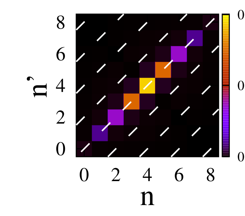
$\gamma_{1}T=\gamma_{2}T=0.5$

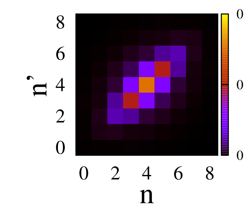
$\gamma_{1}T=\gamma_{2}T=2.0$

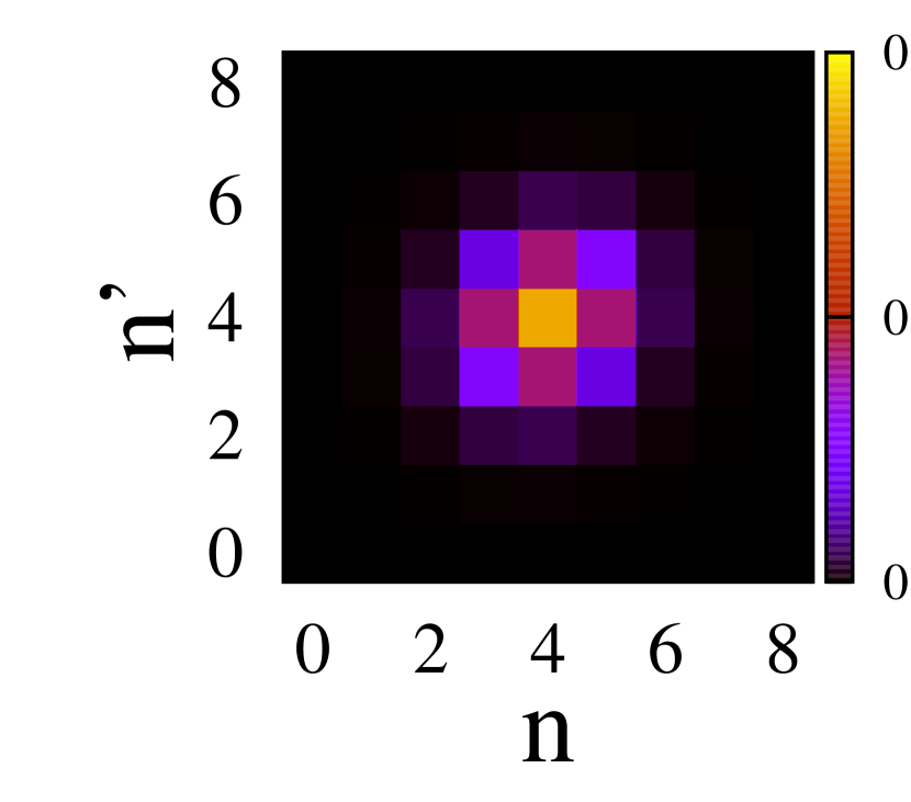
$\gamma_{1}T=\gamma_{2}T=10$

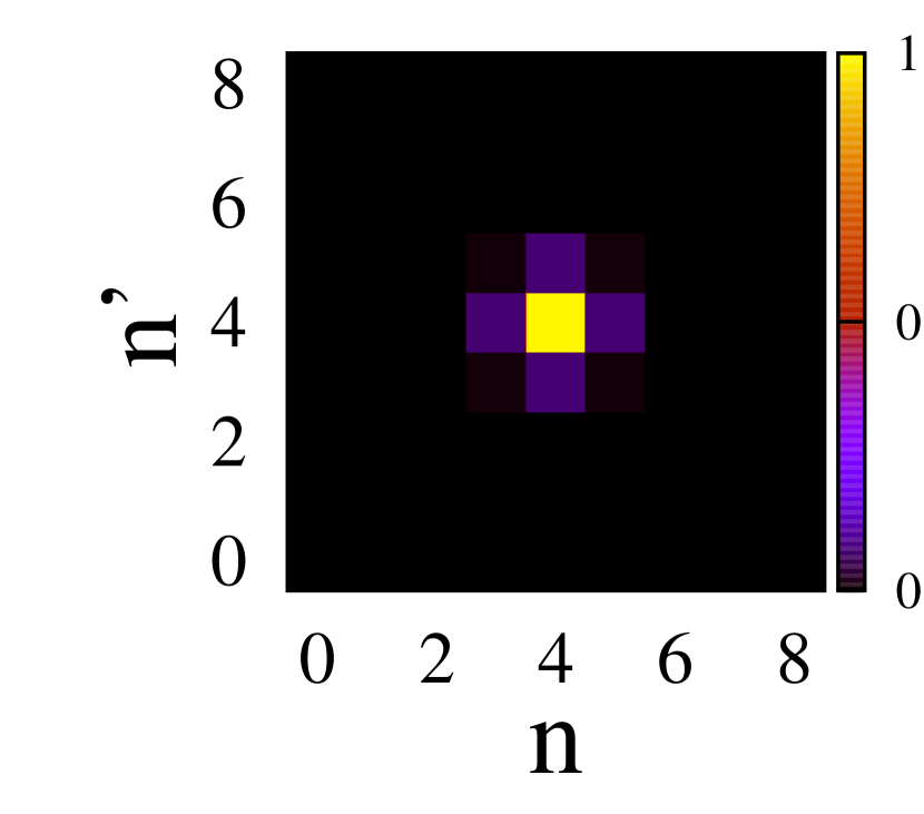
$\gamma_{1}T=0.05$, $\gamma_{2}=0$

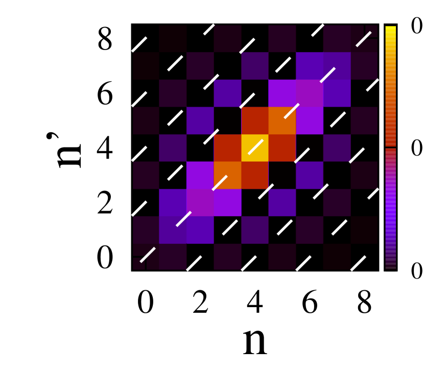
$\gamma_{1}T=1$, $\gamma_{2}=0$

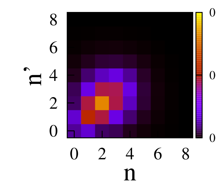
$\gamma_{1}T=4.0$, $\gamma_{2}=0$

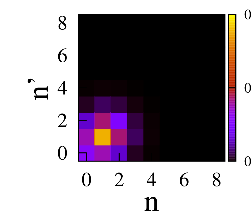
$\gamma_{1}T=20$, $\gamma_{2}=0$

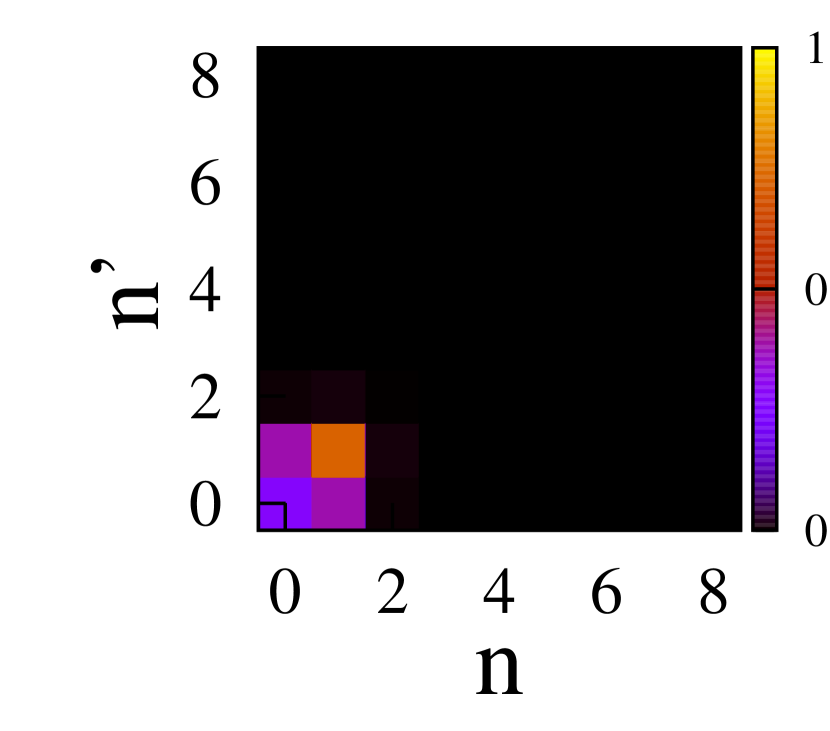
$\gamma_{1}=0$, $\gamma_{2}T=0.05$

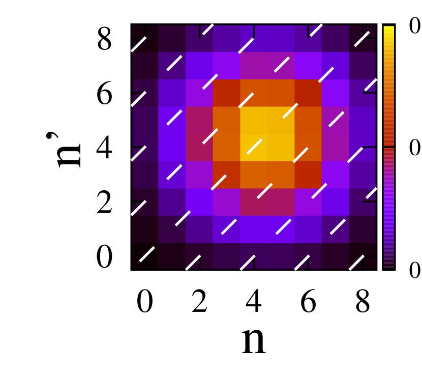
$\gamma_{1}=0$, $\gamma_{2}T=1$

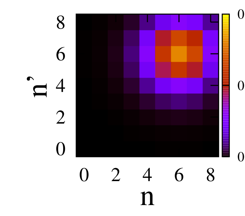
$\gamma_{1}=0$, $\gamma_{2}T=4.0$

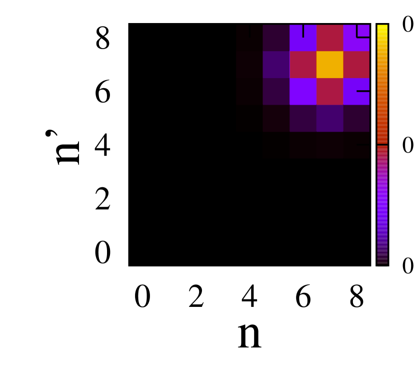
$\gamma_{1}=0$, $\gamma_{2}T=20$

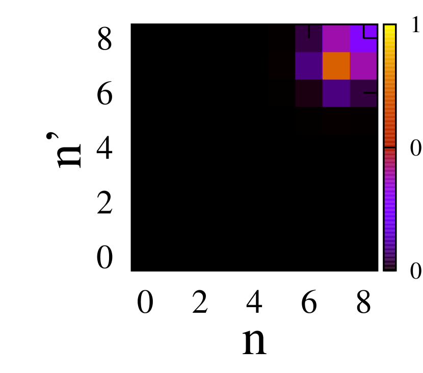
Figure 6: (Color online) Moduli $|\langle n,N_{1}-n|\hat{\rho}_{N_{1}}(t_{2})|n^{\prime},N_{1}-n^{\prime}\rangle|$ of the density matrix in the Fock basis at time $t_{2}=T/4$ in the subspace with $N_{1}=N_{0}-2$ atoms for increasing two-body losses rates (from left to right), from exact diagonalization. The upper panels correspond to symmetric losses and energies ($\gamma_{1}=\gamma_{2}$ and $U_{1}=U_{2}$), the middle panels to asymmetric losses and symmetric energies ($\gamma_{2}=0$ and $U_{1}=U_{2}$), and the bottom panels to asymmetric losses and energies ($\gamma_{1}=0$ and $U_{2}=U_{12}$). The revival time $T$ is the same in all cases. White dashed lines are marking the values of $(n,n^{\prime})$ for which the matrix elements of the diagonal part $[\hat{\rho}^{(0)}(t_{2})]_{\rm d}$ of the two-component superposition do not vanish. Other parameters as in Fig. 4.

IV.3.2 Small loss regime

For small loss rates satisfying

$$\Gamma_{m}\ll N_{0}^{1-r}t^{-1}\quad,\quad r=|m|=1,2,3\;,$$ (44)

the general results of Appendix D take a simpler form which we discuss here. For concreteness we restrict our attention to the times $t=t_{q}$. Let us first observe that one can neglect the $\theta$-noise. In fact, $\delta\theta_{m}$ is much smaller than the quantum fluctuations in the CSs forming the components of the superposition (9) (the latter are of the order of $1/\sqrt{N_{0}}$). In contrast, due to the large fluctuations $\delta s_{m}\approx t_{q}$ of the loss time – which has an almost flat distribution between $0$ and $t_{q}$, the $\phi$-fluctuations are quite large. Indeed, if $\chi_{1}m_{1}+\chi_{2}m_{2}\approx\chi$ then one finds from Eq.(40) that $\delta\phi_{m}$ is of the order of the phase separation $\phi_{k+1,q}-\phi_{k,q}=2\pi/q$ between the CSs.

According to Eqs.(IV.2) and (IV.3.1), for a single $r$-body loss process the conditional state $\hat{\rho}_{N_{1}}^{\rm{(1-jump)}}(t_{q})$ with $N_{1}=N_{0}-r$ atoms is obtained in the Fock basis by multiplying the matrix elements of the superposition $\rho^{(0)}_{N_{1}}(t_{q})$ in the absence of losses by the damping factor

$$D_{q}(n_{1},n_{1}^{\prime})=\exp\Bigl{\{}-\frac{\pi}{\chi q}\bigl{(}d_{N_{1}}(n_{1})+d_{N_{1}}(n_{1}^{\prime})\bigr{)}\Bigr{\}}$$ (45)

and by the envelope (see Eq.(99) in Appendix D)

$${\cal{E}}_{q,r}(n_{1},n_{1}^{\prime})=\frac{q\chi}{\pi}\sum_{|m|=r}\Gamma_{m}C_{m}(t_{q};n_{1},n_{1}^{\prime})\;.$$ (46)

In the last formula, $C_{m}(t_{q};n,n^{\prime})$ is given by Eq.(100) and the factor in front of the sum is put for convenience (then ${\cal{E}}_{q,r}(n_{1},n_{1})=\sum_{|m|=r}\Gamma_{m}$) and disappears in the state normalization. In the limit (44), $C_{m}(t_{q};n,n^{\prime})$ can be approximated for symmetric energies $U_{1}=U_{2}$ (i.e. $\chi_{1}=-\chi_{2}=\chi$) by

$$C_{m}(t_{q};n,n^{\prime})\simeq\frac{1-\exp\bigl{\{}-{\rm{i}}\frac{\pi}{q}(m_{1}-m_{2})(n-n^{\prime})\bigr{\}}}{{\rm{i}}\chi(m_{1}-m_{2})(n-n^{\prime})}\,.$$ (47)

IV.4 Channel effects and protection of quantum correlations against phase noise

In this subsection we study the conditional density matrix $\hat{\rho}_{N_{1}}(t_{q})$ with $N_{1}=N_{0}-r$ atoms for a BJJ subject to a single $r$-body loss event (with $r=1,2$, or $3$), focusing on the times of formation $t=t_{q}$ of the macroscopic superpositions. The more complex case of combined loss processes and several loss events will be discussed in the next subsection. We first single out the peculiar behavior of the Fisher information $F_{N_{1}}(t_{q})$ in the subspace with $N_{1}$ atoms as one varies the loss rates and interaction energies, by relying on the exact diagonalization method. This behavior is then interpreted in the light of the analytical results of Sec. IV.3. We identify several physical effects explaining the different decoherence scenarios discussed in Sec. III for symmetric and asymmetric loss rates and energies.

IV.4.1 Density matrix and quantum Fisher information in the subspace with $N_{0}-2$ atoms

Let us start by presenting the amount of QCs in the subspace with $N_{1}$ atoms calculated from the exact diagonalization method. We restrict ourselves here to two-body losses, assuming no one-body, three-body, and inter-mode losses (i.e. $\alpha_{i}=\gamma_{12}=\kappa_{i}=\kappa_{ij}=0$). The density matrix $\hat{\rho}_{N_{1}}(t_{2})$ in the Fock basis is shown in Fig. 6. If the interaction energies in the two modes are equal, i.e. $U_{1}=U_{2}$, we observe that $\hat{\rho}_{N_{1}}(t_{2})$ is almost diagonal in the Fock basis for weak symmetric loss rates $\gamma_{1}=\gamma_{2}\lesssim\chi/N_{0}$ (upper left panel), while it has non-vanishing off-diagonal elements for odd values of $n_{1}^{\prime}-n_{1}$ for completely asymmetric rates $\gamma_{2}=0$ (middle left panel). Moreover, if one takes $\gamma_{1}=0$ in the first mode and tunes the energies such that $U_{2}=U_{12}$, keeping $\chi=(U_{1}+U_{2}-2U_{12})/2$ fixed, the density matrix has the same structure as that of a two-component superposition with $N_{1}=N_{0}-2$ atoms (lower left panel). This is confirmed by looking at the Fisher information $F_{N_{1}}(t_{2})$, which is displayed in Fig. 7. We stress that, unlike in Fig. 2, this Fisher information is not multiplied by the one-jump probability $w_{N_{1}}(t_{q})$ and the optimization over the interferometer direction $\vec{n}$ is done in the $N_{1}$-atom sector, independently of the other sectors. If one of the modes does not lose atoms and $U_{i}=U_{12}$ in the other mode (Fig. 2b), $F_{N_{1}}(t_{2})$ is approximately equal for $\gamma_{1}\ll\chi/N_{0}$ to the Fisher information $N_{1}^{2}$ of a two-component superposition. At stronger loss rates $\gamma_{1}\approx 1/T=\chi/(2\pi)$, $F_{N_{1}}(t_{2})$ decreases to much lower values. In contrast, for symmetric losses and energies, $F_{N_{1}}(t_{2})$ starts below the shot-noise limit at weak losses and increases with $\gamma_{1}$ to reach a maximum when $\gamma_{1}\simeq 2/T$. As we will see below, these different behaviors of the Fisher information for symmetric and asymmetric loss rates and energies occur in all subspaces with $N<N_{0}$ atoms and for all types of losses, thereby explaining the differences in the total Fisher information presented in Sec. III.

We now turn to the quantum jump approach. By analyzing the form of the envelope (46) in the small loss regime, we argue below that the aforementioned behavior of $F_{N_{1}}(t_{q})$ comes mainly from the combination of two effects: a channel effect for $U_{1}=U_{2}$ and $q=2,3$, and the suppression of phase noise in the $i$th loss channel when $U_{i}=U_{12}$. Before discussing these two effects, we show that for $U_{1}=U_{2}$ the phase noise always induces a complete phase relaxation in the weak loss regime. However, we emphasize that this phase relaxation is not relevant for the Fisher information.

a) symmetric loss rates ($\gamma_{1}=\gamma_{2}$)

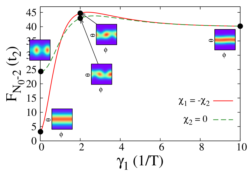
b) asymmetric loss rates ($\gamma_{2}=0$)

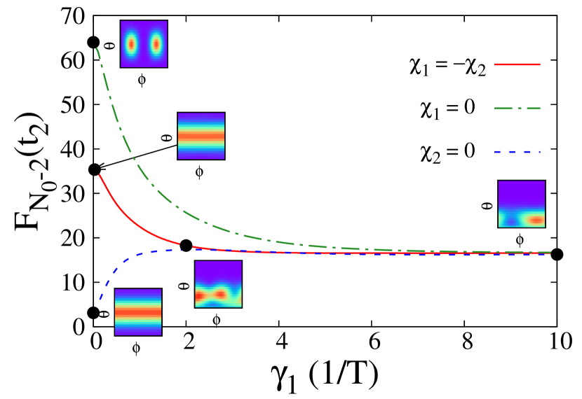
Figure 7: (Color online) Quantum Fisher information optimized in the subspace with $(N_{0}-2)$ atoms at time $t_{2}$ as a function of the two-body loss rate (in units of $T^{-1}$) for (a) symmetric losses $\gamma_{1}=\gamma_{2}$ with $U_{1}=U_{2}$ (red solid line) and $U_{2}=U_{12}$ (green dashed line); (b) completely asymmetric losses with $\gamma_{2}=0$ and $U_{1}=U_{2}$ (red solid line), $U_{1}=U_{12}$ (green dot dashed line), and $U_{2}=U_{12}$ (blue dashed line). The $U_{i}$ are chosen in such a way that the revival time $T$ does not change. Insets: plots of the Husimi functions for some specific choices of loss rates (indicated by circles and arrows). Other parameters as in Fig. 4. All results are obtained from the exact diagonalization method.

IV.4.2 Complete phase relaxation for $U_{1}=U_{2}$

Let us study the impact of the phase noise on $\hat{\rho}_{N_{1}}(t_{q})$ for symmetric interaction energies $U_{1}=U_{2}$ (i.e. $\chi_{1}=-\chi_{2}=\chi$) and small loss rates satisfying (44). Then $\delta s_{m}\approx t_{q}$ and Eq.(40) gives $\delta\phi_{m}\approx|m_{1}-m_{2}|\pi/q$. This implies that phase noise due to losses with unequal numbers of atoms $m_{i}$ in each mode $i$ blurs out the phases of the CSs, whereas a loss of one atom in each mode does not modify the state.

Before showing this explicitly, let us mention some results established in ferrini2010a ; ferrini2010 concerning the effect of phase noise on macroscopic superpositions in BJJs. We recall that one can decompose the density matrix as a sum of its diagonal and off-diagonal parts defined in Eq.(II.1.2). This can also be done in the presence of noise. Phase noise flattens the Husimi distribution of the superposition in the $\phi$ direction (phase relaxation), which manifests itself by the convergence for strong noise of the diagonal part of the density matrix to a statistical mixture of Fock states with completely undefined phases. A second effect of phase noise is the loss of the coherences between the CSs of the superposition, leading to a convergence of the off-diagonal part to zero at strong noises. This off-diagonal part, albeit it does not influence the Husimi distribution, contains the QCs useful for interferometry. It was pointed out in ferrini2010a ; ferrini2010 that for intermediate phase noise one may have almost complete phase relaxation while some QCs remain (weak decoherence).

In our case, the action of phase noise on the diagonal and off-diagonal parts of $\hat{\rho}_{N_{1}}(t_{q})$ can be evaluated exactly. From Eqs.(13), (IV.2), and (IV.3.1), the matrix elements of $[\hat{\rho}_{N_{1}}(t_{q})]_{\rm d}$ in the Fock basis vanish for $n_{1}^{\prime}\not=n_{1}$ modulo $q$. We may thus restrict our attention to $n_{1}^{\prime}=n_{1}+pq$ for integer $p$’s. Due to Eqs.(46) and (47), if $p\not=0$ then the envelope reads

$${\cal{E}}_{q,r}(n_{1},n_{1}+pq)\simeq\begin{cases}-{\rm{i}}\Delta\alpha\frac{1-(-1)^{p}}{\pi p}&\text{for $r=1$}\\ \gamma_{12}&\text{for $r=2$}\\ -{\rm{i}}(\Delta\kappa+3\Delta\kappa_{12})\frac{1-(-1)^{p}}{3\pi p}&\text{for $r=3$}\end{cases}$$ (48)

with $\Delta\alpha=\alpha_{2}-\alpha_{1}$, $\Delta\kappa=\kappa_{2}-\kappa_{1}$, and $\Delta\kappa_{12}=\kappa_{21}-\kappa_{12}$. Therefore, for weak two-body losses and in the absence of inter-mode losses the diagonal part is equal to a statistical mixture of Fock states,

$$\langle n_{1},N_{1}-n_{1}|\,[\hat{\rho}_{N_{1}}(t_{q})]_{\rm d}|n_{1}^{\prime},N_{1}-n_{1}^{\prime}\rangle$$

$$\hskip 56.9055pt\propto\;\delta_{n_{1},n_{1}^{\prime}}\left(\begin{array}[]{c}N_{1}\\ n_{1}\end{array}\right)e^{-\frac{2\pi}{\chi q}d_{N_{1}}(n_{1})}\;,$$ (51)

where we have used Eqs.(10), (45), and (46). This is confirmed in the upper and middle left panels in Fig. 6, where one observes vanishing matrix elements along the dashed lines $n_{1}^{\prime}=n_{1}\pm 2$, $n_{1}^{\prime}=n_{1}\pm 4,\ldots$. We thus find that the loss of two atoms in the same mode leads to complete phase relaxation. This explains the $\phi$-independent profile of the Husimi distributions in the insets in Fig. 7 corresponding to $\chi_{1}=-\chi_{2}$ and $\gamma_{1}\ll 1/(TN_{0})$. In contrast, no phase relaxation occurs in the inter-mode channel $m=(1,1)$.

For one- and three-body losses, complete phase relaxation occurs for symmetric losses ($\alpha_{1}=\alpha_{2}$, $\kappa_{1}=\kappa_{2}$, and $\kappa_{12}=\kappa_{21}$) only. This can be understood intuitively as follows. For weak losses the random phase $\phi_{1,0}=s\chi$ ($\phi_{0,1}=-s\chi$) produced by the loss of one atom in the mode $i=1$ ($i=2$) is uniformly distributed in $[0,\pi/q]$ ($[-\pi/q,0]$). Since the components of the superposition have a phase separation of $2\pi/q$, it is clear that one needs equal loss probabilities in the two modes to wash out its phase content completely. Note that here complete phase relaxation comes from an exact cancellation when adding the contributions of the two loss channels $m=(1,0)$ and $m=(0,1)$, which separately lead to non-diagonal matrices $[\hat{\rho}_{N_{1}}(t_{q})]_{\rm d}$. A similar argument applies to three-body losses.

IV.4.3 Loss of quantum correlations when $U_{1}=U_{2}$ and $q=2$ or $3$: channels effects

As discussed above, the phenomenon of phase relaxation does not tell us anything about the QCs useful for interferometry, which can still be present in the atomic state even if one has complete phase relaxation. Let us now study these QCs, contained in the off-diagonal part $[\hat{\rho}_{N_{1}}(t_{q})]_{\rm od}$ of the conditional state. We still assume symmetric energies $U_{1}=U_{2}$ and small losses satisfying (44). The off-diagonal part corresponds to the matrix elements of $\hat{\rho}_{N_{1}}(t_{q})$ in the Fock basis such that $n_{1}^{\prime}\not=n_{1}$ modulo $q$ (see Eq.(13)). In view of Eq.(47), the main effect of phase noise is to multiply the matrix elements in the absence of noise by a factor of $(n_{1}-n_{1}^{\prime})^{-1}$. This factor decays to zero as one moves away from the diagonal but does not modify substantially the elements close to the diagonal. This explains the presence of off-diagonal matrix elements for $n_{1}^{\prime}=n_{1}\pm 1$ and $n_{1}^{\prime}=n_{1}\pm 3$ in Fig. 6 when $\gamma_{1}\ll\chi/N_{0}$, $\gamma_{2}=0$, and $U_{1}=U_{2}$ (left middle panel), as well as the relatively high value of the Fisher information $F_{N_{0}-2}(t_{2})$ in Fig. 7(b). For such loss rates and energies we are in the noise regime of the aforementioned weak decoherence, i.e. phase noise is more efficient in washing out the phase content of each component of the superposition than in destroying the coherences.

However, we see in Figs. 6 and 7 that the situation is quite different for symmetric two-body losses $\gamma_{1}=\gamma_{2}$ and $\gamma_{12}=0$: then $[\hat{\rho}_{N_{1}}(t_{2})]_{\rm od}$ vanishes completely and the Fisher information at weak losses is smaller than $N_{0}$. This comes from a cancellation when adding the contributions of the $m=(2,0)$ and $m=(0,2)$ loss channels, which occurs only at time $t_{2}$ and in the absence of inter-mode losses. A similar cancellation occurs at time $t_{3}$ when the two modes are subject to three-body losses with symmetric rates $\kappa_{1}=\kappa_{2}$ and $\kappa_{12}=\kappa_{21}=0$. In fact, for such loss rates Eqs.(46) and (47) yield ${\cal{E}}_{r,r}(n,n^{\prime})\simeq 2\Gamma_{r,0}\delta_{n,n^{\prime}}$ for $r=2,3$. Hence $[\hat{\rho}_{N_{1}}(t_{2})]_{\rm od}=0$, so that the whole density matrix $\hat{\rho}_{N_{1}}(t_{2})$ is diagonal in the Fock basis and given by Eq.(IV.4.2). This is clearly seen in the upper left panel in Fig. 6. As a consequence of this channel effect, the two-component (three-component) superposition suffers in the absence of inter-mode losses from a complete decoherence in the $N_{1}$-atom subspace, for arbitrary small symmetric two-body (three-body) loss rates. Note that this is not in contradiction with the fact that the total state $\hat{\rho}(t_{2})$ converges to $\hat{\rho}^{(0)}(t_{2})$ when $\Gamma_{m}\rightarrow 0$, since the probability $w_{N_{1}}(t_{2})$ converges to zero in this limit and thus $\hat{\rho}_{N_{1}}(t_{2})$ does not contribute to the total state. Such a channel effect does of course not occur for completely asymmetric losses involving only one channel. It is illustrated in Fig. 8, which displays the Fisher information $F_{N_{1}}(t)$ as a function of time. For asymmetric losses, $F_{N_{1}}(t)$ is maximum at time $t_{2}$ as in the lossless case. For symmetric two-body losses, instead, $F_{N_{1}}(t)$ is minimum at $t_{2}$ due to the channel effect.

We emphasize that symmetric one-body losses $\alpha_{1}=\alpha_{2}$ and inter-mode three-body losses $\kappa_{12}=\kappa_{21}$ do not produce any channel effect. This means that these loss processes are less detrimental to the macroscopic superpositions than symmetric two-body losses. For instance, one has ${\cal{E}}_{q,1}(n,n^{\prime})=2\alpha_{1}\operatorname{sinc}[\pi(n-n^{\prime})/q]$ for $\alpha_{1}=\alpha_{2}$ (we remind that we are treating for the moment the case of symmetric interactions $U_{1}=U_{2}$). A striking consequence of this observation will be discussed in Sec. IV.5.1 below.

IV.4.4 Protecting macroscopic superpositions by tuning the interaction energies

Let us now proceed to the case of asymmetric interaction energies $U_{1}\not=U_{2}$. In order to keep the formation time $t_{q}=\pi/(\chi q)$ of the superposition constant, we vary $U_{1}$ and $U_{2}$ while fixing $2\chi=\chi_{1}-\chi_{2}$. We still consider weak losses satisfying (44). Then the phase relaxation described above is incomplete, as well as decoherence at times $t_{2}$ or $t_{3}$ for symmetric losses. An interesting situation is $U_{2}=U_{12}<U_{1}$, i.e. $\chi_{2}=0$ and $\chi_{1}=2\chi$. Then $\phi_{0,r}(s)=0$ by Eq.(IV.3.1), thus the second mode is protected against phase noise, whereas the first mode is subject to a strong noise with fluctuations $\delta\phi_{r,0}\approx 2\pi r/q$. Taking for simplicity vanishing inter-mode rates, one gets from Eq.(46) and from Eq.(100) in Appendix D

$${\cal{E}}_{q,r}(n,n^{\prime})=\Gamma_{0,r}+q\Gamma_{r,0}\frac{1-\exp\{-{\rm{i}}\frac{2\pi r}{q}(n-n^{\prime})\}}{2{\rm{i}}\pi r(n-n^{\prime})}\;.$$ (52)

For symmetric rates $\Gamma_{0,r}=\Gamma_{r,0}$, the off-diagonal matrix elements of $\hat{\rho}_{N_{1}}(t_{2})$ in the Fock basis coincide with those of a two-component superposition up to a factor of the order of $1/2$. Loosely speaking, $\hat{\rho}_{N_{1}}(t_{2})$ is a “half macroscopic superposition”. Such a state has a large Fisher information, as shown in Fig. 7(a). An even larger Fisher information is obtained for completely asymmetric losses with $\Gamma_{r,0}=0$, i.e. if atoms are lost in the protected mode $i=2$ only. Then ${\cal{E}}_{q,r}(n,n^{\prime})=\Gamma_{0,r}$ and $\hat{\rho}_{N_{1}}(t_{q})\propto\widetilde{\rho}_{N_{1}}^{\rm{(no\,loss)}}(t_{q})$, that is, the conditional state $\hat{\rho}_{N_{1}}(t_{q})$ coincides with a superposition of $q$ CSs with $N_{1}$ atoms, slightly modified by the damping factor (45). This is in agreement with the convergence at weak losses and asymmetric energies of the Fisher information $F_{N_{0}-2}(t_{2})$ in Fig 7(b) to the highest possible value $(N_{0}-2)^{2}$, and to the presence of two well-pronounced peaks at $\phi=\pm\pi/2$ in the corresponding Husimi distributions.

In summary, by tuning the interaction energies $U_{i}$ such that $\chi_{1}=0$ or $\chi_{2}=0$ one can protect one mode against phase noise, to the expense of enlarging noise in the other mode, thereby limiting decoherence effects on the conditional state with $N_{1}$ atoms. This way of switching phase noise off in one mode has been pointed out in pawlowski2013 for two-body losses. As a central result we find here that it applies to one- and three-body losses as well. One can similarly switch the phase noise off in the two-body inter-mode loss channel $m=(1,1)$ by tuning the energies such that $\chi_{2}=-\chi_{1}$ (i.e. by taking symmetric energies $U_{1}=U_{2}$) and in the three-body inter-mode loss channels $m=(2,1)$ and $(1,2)$ by taking $\chi_{2}=-2\chi_{1}$ and $\chi_{1}=-2\chi_{2}$ (i.e. $U_{1}=U_{2}\mp 2\chi/3$), respectively. We emphasize that it is impossible to suppress the noise in two different loss channels at the same time. Therefore, the optimal energy tuning for protecting the macroscopic superpositions is to switch phase noise off in the channel losing more atoms.

To complete the description of Fig. 7 we discuss in what follows three effects of atom losses occurring at intermediate and strong loss rates.

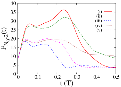
Figure 8: (Color online) Quantum Fisher information optimized in the subspace with $N_{0}-2$ atoms versus time for symmetric energies $U_{1}=U_{2}$, from exact diagonalization. The red solid and green dashed lines (upper curves) correspond to asymmetric two-body losses with (i) $\gamma_{1}T=0.05$, $\gamma_{2}=0$ and (ii) $\gamma_{1}T=1.0$, $\gamma_{2}=0$. The blue dot-dashed, brown dotted and magenta dot-dashed lines (lower curves) correspond to symmetric two- and one-body losses with (iii) $\gamma_{1}=\gamma_{2}=0.025/T$, $\alpha_{i}=0$, (iv) $\gamma_{1}=\gamma_{2}=0.5/T$, $\alpha_{i}=0$, and (v) $\gamma_{1}=\gamma_{2}=0.025/T$, $\alpha_{1}=\alpha_{2}=0.5/T$. Other parameters: $N_{0}=10$ and $\gamma_{12}=\kappa_{i}=\kappa_{ij}=0$.

IV.4.5 Increasing the loss rates reduces phase noise

We first study the regime of intermediate loss rates. Surprisingly, the $\phi$-noise decreases if one increases $\Gamma_{m}$. This results from the decrease of the loss time fluctuations $\delta s_{m}$ at increasing $\Gamma_{m}$, leading to a decrease of the phase fluctuations $\delta\phi_{m}$ in Eq.(40). In fact, while for small rates the loss time is uniformly distributed on the interval $[0,t_{q}]$, for larger rates the loss has more chance to occur at small times and $\delta s_{m}$ gets smaller. For instance, it is easy to see by inspection of the distribution (97) in Appendix D that $\delta s_{m}\simeq G_{m}^{-1}$ when $G_{m}\gtrsim\chi q$ and $N_{0}\gg 1$, $G_{m}$ being a non-decreasing function of the rates $\Gamma_{m}$ given by Eq.(86). This decreasing of the phase noise sets in for $G_{m}\approx\chi q$, that is, $\Gamma_{m}\approx\chi qN_{0}^{1-|m|}$. Therefore, by increasing the loss rates one protects the conditional state with $N_{1}$ atoms against phase noise and thus against decoherence. As seen in Fig. 2, this counter-intuitive effect does not manifest itself in the total Fisher information $F_{\rm tot}(t)$. Indeed, when increasing $\gamma_{1}$ the subspaces contributing to $F_{\rm tot}(t)$ in Eq.(19) have less atoms and hence are less quantum correlated, and the increase of $F_{N_{0}-2}(t)$ is counter-balanced by the decrease of the probability $w_{N_{0}-2}(t)$. As a consequence, $F_{\rm tot}(t)$ is getting smaller.

IV.4.6 Effect of the $\theta$-noise

The fact that the peaks of the Husimi distributions in Fig. 7(b) at intermediate losses are centered at values of $\theta$ smaller than $\pi/2$ is due to the $\theta$-noise. In fact, in this figure $\delta_{1}=2\gamma_{1}>0$ and $\delta_{2}=0$, so that $\theta_{2,0}(s)<\pi/2$ and $\theta_{0,2}(s)=\pi/2$. For larger initial atom numbers $N_{0}$ the $\theta$-noise is always small, its fluctuations being of the order of $1/N_{0}$ when $N_{0}\gg 1$. Actually, when $G_{m}\gtrsim\chi q$ one finds $\delta\theta_{m}\approx 1/N_{0}$ by replacing $\delta s_{m}$ by $G_{m}^{-1}$ in Eq.(40), whereas for $G_{m}<\chi q$ one has $\delta\theta_{m}<t_{q}r\max\{|\delta_{1}|,|\delta_{2}|\}/2$.

IV.4.7 Damping effects

Increasing further the rates $\Gamma_{m}$, the damping due to the effective Hamiltonian begins to play the major role. The combination of this damping with the reduced phase noise effect described above leads again to different behaviors of $F_{N_{1}}(t_{q})$ as a function of the loss rates for symmetric and asymmetric losses. Let us recall from Sec. IV.2 that the onset of damping is for $\Gamma_{m}\approx\chi qN_{0}^{1-|m|}$ in the symmetric case and $\Gamma_{m}\approx\chi qN_{0}^{-|m|}$ in the asymmetric case. On the other hand, we have seen above that phase noise reduction begins when $\Gamma_{m}\approx\chi qN_{0}^{1-|m|}$. For symmetric losses, there exists a small range of loss rates $\Gamma_{m}$ on which phase noise is reduced by increasing $\Gamma_{m}$ while the damping is still relatively small. This explains the increase of $F_{N_{1}}(t_{2})$ with $\gamma_{1}$ seen in Fig. 7(a). At the point where $F_{N_{1}}(t_{2})$ reaches a maximum, two peaks are clearly visible in the Husimi distribution, as opposed to the flat distribution observed at weak losses. This nicely illustrates phase noise reduction. In contrast, in the asymmetric case damping effects counter-balance phase noise reduction and the Fisher information decreases when increasing $\gamma_{1}$ (even though some peaks show up in the Husimi plots). For $\gamma_{1}=\gamma_{2}\gg\chi$ and even initial atom numbers $N_{0}$, $\hat{\rho}_{N_{0}-2}(t_{q})$ converges to a Fock state with $(N_{0}-2)/2$ atoms in each mode, which has a high Fisher information $(N_{0}-2)N_{0}/2$ (see Appendix C). For asymmetric losses, instead, $\hat{\rho}_{N_{0}-2}(t_{q})$ converges to a superposition of Fock states with $n_{1}=0$ or $1$ atom in the first mode, and $F_{N_{0}-2}(t_{2})\approx N_{0}$, as seen in Fig. 7(b). Similarly, the comparison of the two first rows in Fig. 6 shows that an increase of $\gamma_{1}=\gamma_{2}$ makes non-vanishing off-diagonal matrix elements to appear, as a consequence of phase noise reduction, while for $\gamma_{2}=0$ the same operation moves the peak in the density matrix towards $n_{1}=n_{1}^{\prime}=0$, as a consequence of damping.

Let us stress again that these effects on the conditional state with $N_{1}$ atoms at strong losses do not affect the total density matrix because of the small probability to have a single loss event between $t=0$ and $t=t_{q}$. Note also that the approximations made in Sec. IV.3 break down for strong losses, namely, Eq.(IV.3.1) is still valid but the envelope ${\cal E}_{N}$ has a more complex expression than that given in Eq.(43) (see Appendix D). Since for $\Gamma_{m}\gg\chi N_{0}^{1-|m|}$ the most important effect is damping, the precise form of ${\cal E}_{N}$ does, however, not matter.

IV.5 Conditional states for several loss events

We can now extend the previous results to the case of several loss events. In view of Eq.(43) the physical effects discussed above are present in all subspaces with $N$ atoms, provided that $0<N_{0}-N\ll N_{0}$. However, some of our conclusions for a single loss event must be modified because of the combination of the different loss processes.

IV.5.1 Suppression of the channel effect due to one-body losses

The channel effect leading to complete decoherence at times $t_{2}$ or $t_{3}$ for weak symmetric losses is suppressed if, in addition to two- or three-body losses, also one-body losses are present. In fact, the density matrix in the subspace with $N_{0}-r$ atoms, $r=2$ or $3$, is given by Eq.(IV.3.1) with an envelope ${\mathcal{E}}_{N_{0}-r}(t_{r};n,n^{\prime})\propto{\mathcal{E}}_{r,r}(n,n^{\prime})+[{\mathcal{E}}_{r,1}(n,n^{\prime})]^{r}/r!$, see Eq.(43). As pointed out in Sec. IV.4.3, ${\mathcal{E}}_{r,r}(n,n^{\prime})$ vanishes for $n\not=n^{\prime}$ (channel effect), but this is not the case for the envelope ${\mathcal{E}}_{r,1}(n,n^{\prime})$ coming from one-body losses. We thus find that by adding one-body losses one can reduce decoherence on the two-component or the three-component superpositions. We have checked that off-diagonal elements indeed appear in the density matrix $\hat{\rho}_{N_{0}-2}(t_{2})$ displayed in the upper left panel in Fig. 6 when one adds one-body losses. A surprising consequence of these off-diagonal elements is shown in Fig. 8: if one-body losses are added to the two-body losses, the Fisher information $F_{N_{0}-2}(t_{2})$ increases in spite of the larger amount of losses. This does, however, not affect the total Fisher information. Indeed, we have always observed numerically a decrease of $F_{\rm tot}(t)$ when one-body losses are added.

IV.5.2 Tuning the interaction energies

For strongly asymmetric loss rates, as in the case of a single loss event it is possible to protect the QCs in the atomic state by tuning the interaction energies while keeping fixed the energy $\chi$ governing the lossless dynamics. However, if the loss rates are symmetric, decoherence effects are strong when many loss events occur between times $0$ and $t_{q}$, whatever the choice of the energies. The argument goes as follows. If all losses occur mostly in the same mode $i$, one can switch phase noise off in that mode $i$ by tuning the atomic energies in such a way that $\chi_{i}=0$ (see Sec. IV.4.4). Then each conditional state $\hat{\rho}_{N}(t_{q})$, with $N_{0}-N\ll N_{0}$, is close to a $q$-component superposition with $N$ atoms, apart from small damping effects. This comes from the product form (43) of the envelope ${\cal{E}}_{N}$ in Eq.(IV.3.1) and from our previous results on the envelope ${\cal{E}}_{q,r}(n,n^{\prime})$ for single loss events, which is almost constant for weak loss rates $\Gamma_{m}\ll q\chi N_{0}^{1-|m|}$. The same statement holds if losses occur mainly via inter-mode two-body processes (i.e. $\gamma_{12}\gg\gamma_{i},\alpha_{i}/N_{0},\kappa_{i}N_{0},\kappa_{ij}N_{0}$); then one must tune the energies such that $U_{1}=U_{2}$. For symmetric losses the situation is different. As soon as the number $N_{0}-N$ of lost atoms becomes large, the tuning of the energies $U_{i}$ is inefficient to keep the coherences of the superposition, because the probability that all losses occur in the same mode decreases exponentially with the number of loss events. Actually, we have seen above that only one mode can be protected against phase noise if $\chi$ is kept constant. Therefore, when a large number of atoms leave the BJJ, the loss rates must be strongly asymmetric in order to be able to protect efficiently the superpositions from decoherence by tuning the $U_{i}$. These results provide a good explanation of the effects described in Figs. 2 and 3.

In order to fully explain the high values of the total Fisher information at time $t_{q}$ for strongly asymmetric losses found in Sec. III, we must also show that the interferometer direction $\vec{n}$ optimizing the Fisher information $F(\hat{\rho}_{N}(t_{q}),\hat{J}_{\vec{n}})$ in the $N$-atom subspace is almost the same for all $N$ (otherwise one could not take advantage of the QCs to improve the phase precision of the interferometer when the number of atoms at time $t_{q}$ is unknown). To see that this is indeed the case, let us note that the optimal directions roughly coincide with one of the phases $\phi_{k,q}$ of the superposition (9), which are given by (we assume here $E_{1}=E_{2}$)

$$\phi_{k,q}=\Bigl{[}2k+\epsilon_{q}-N+\chi^{-1}(N-1)\frac{U_{2}-U_{1}}{2}\Bigr{]}\frac{\pi}{q}$$ (53)

with $\epsilon_{q}=0$ if $q$ is even and $1$ otherwise. When $U_{2}=U_{12}$ (or $U_{1}=U_{12}$) we obtain $\phi_{k,q}=[2k+\epsilon_{q}-2N+1]\pi/q$ (or $\phi_{k,q}=[2k+\epsilon_{q}-1]\pi/q$). Thus the components of the superpositions are transformed one into another by changing $N$ (for $q$ fixed) and the optimal directions are the same. One deduces from this argument that the total Fisher information $F_{\rm tot}(t_{q})$ in Eq.(19) is close to the Fisher information of a $q$-component superposition with $\langle\hat{N}\rangle_{t_{q}}$ atoms, and thus scale like $\langle N\rangle^{2}_{t_{q}}$, where $\langle\hat{N}\rangle_{t_{q}}$ is the average number of atoms at time $t_{q}$.

IV.6 Dependence of the Fisher information on the initial atom number $N_{0}$

Let us briefly discuss the effect of an increase of the initial number of atoms $N_{0}$ on the QCs in the macroscopic superpositions, focusing on the completely asymmetric loss case $\alpha_{1}=\gamma_{1}=\kappa_{1}=0$ and no inter-mode losses. The increase of $N_{0}$ leads to a rapid increase of the probability for losing atoms. Indeed, for large $N_{0}$ the mean number $\langle N\rangle_{t_{q}}$ of atoms in the BJJ at time $t_{q}$ behaves like $N_{0}(\gamma_{2}N_{0}t_{q}+1)^{-1}$ for two-body losses and $N_{0}(2\kappa_{2}N_{0}^{2}t_{q}+1)^{-1/2}$ for three-body losses, as follows from the phenomenological rate equations.

We first consider the case of asymmetric interaction energies $U_{2}=U_{12}<U_{1}$. If $N_{0}$ is small enough so that the BJJ remains in the weak loss regime $\alpha_{2}\ll\chi q$, $\gamma_{2}N_{0}\ll\chi q$, and $\kappa_{2}N_{0}^{2}\ll\chi q$, it has been argued above that the total Fisher information $F_{\rm tot}(t_{q})$ should scale like $\langle N\rangle^{2}_{t_{q}}\approx N_{0}^{2}$. However, when $\gamma_{2}N_{0}^{2}$ and $\kappa_{2}N_{0}^{3}$ become of the order of $\chi q$ one expects a less pronounced increase of $F_{\rm tot}(t_{q})$ with $N_{0}$ because of the damping effects discussed in Secs. IV.2 and IV.4.7, as confirmed by a comparison of Fig. 2(a) and Fig. 3. Increasing further $N_{0}$, one enters into the intermediate loss rate regime with $\gamma_{2}N_{0}\approx\chi q$ and $\kappa_{2}N^{2}_{0}\approx\chi q$, characterized by a non negligible fraction of lost atoms, strong damping, and much stronger decoherence effects.

Let us now take symmetric energies $U_{1}=U_{2}$. In the weak loss regime the envelope in Eq.(IV.3.1) decays like $(n_{1}-n_{1}^{\prime})^{-J_{1}-J_{2}-J_{3}}$ as one moves away from the diagonal $n_{1}=n_{1}^{\prime}$, see (43), (46), and (47). Thus, as the number $N_{0}-N=J_{1}+2J_{2}+J_{3}$ of lost atoms is getting larger the conditional states $\hat{\rho}_{N}(t_{q})$ become more diagonal in the Fock basis, in contrast with what happens for asymmetric energies. By increasing $N_{0}$, the mean number of lost atoms increases and the total atomic state $\hat{\rho}(t_{q})$ gets closer to a statistical mixture of Fock states, leading to a disappearance of the QCs in the macroscopic superposition. It should be noted, however, that for fixed numbers of jumps $J_{1}$, $J_{2}$, and $J_{3}$, the decay of the off-diagonal elements of the conditional states $\hat{\rho}_{N}(t_{q})$ in the Fock basis is the same for all $N_{0}$. This is related to the fact that in a BJJ subject to phase noise the decoherence time is independent of the number of atoms ferrini2010a . Hence some QCs remain in the conditional states $\hat{\rho}_{N}(t_{q})$ even for large $N_{0}$. The degradation of the QCs in the total state results from the decay of the probabilities $w_{N}(t_{q})$ to have $N$ atoms at time $t_{q}$. The behavior of the Fisher information $F_{\rm tot}(t_{q})$ as a function of $N_{0}$ strongly depends on the behavior of these probabilities.

V Summary and concluding remarks

We have studied in detail the decoherence induced by one-, two- and three-body atom losses on the superpositions of coherent states dynamically generated in BJJs. For all loss types and at weak losses, the degradation of the superposition is mainly due to a strong effective phase noise and to a channel effect. The last effect gives rise to enhanced decoherence on the two-component (three-component) superposition after summing over the two loss channels when the two-body (three-body) loss rates and interaction energies are the same in the two modes and there are no inter-mode losses. Conversely, if all losses occur mostly in one mode, we have shown that it is possible to partially prevent this degradation by adjusting the interaction energy $U_{i}$ of each mode, keeping their sum fixed and exploiting the experimental tunability of $U_{i}$. For instance, in the absence of inter-mode losses the effective phase noise can be suppressed in the mode loosing more atoms by choosing an interaction energy in this mode equal to the inter-mode interaction $U_{12}$. For internal BJJs with Rubidium atoms as used in Ref. gross2010 , this could be done by reducing the scattering length $a_{1}$ in the mode $i=1$ loosing less atoms. Then, because $a_{2}$ and $a_{12}$ are almost equal, one has $U_{2}\simeq U_{12}$, whereas $|U_{1}-U_{12}|$ can be large. For experimentally relevant loss rates and initial atom numbers, we have found that the amount of coherence left at the time of formation of the two-component superposition can be made in this way substantially higher, provided that the system has strongly asymmetric losses (see Fig. 3). In the experiment of Ref. gross2010 , this condition is met for two-body losses but not for one-body losses, which are symmetric in the two modes. As a consequence, in the range of parameters corresponding to the experimental situation that we have studied, we predict that one-body loss processes lead to much stronger decoherence effects on the macroscopic superposition than the asymmetric two-body processes.

Appendix A Solution of the master equation by the exact diagonalization method

We present in this appendix the exact solution of the master equation (14) with Lindblad generators (II.1.3) in the absence of inter-mode losses. In the notation of Sec. II.1 this means $\kappa_{21}=\kappa_{12}=\gamma_{12}=0$. The loss rates in the first and second modes are denoted as in Sec. II.3 by $\Gamma_{r,0}$ and $\Gamma_{0,r}$, respectively, with $r=1$, $2$, and $3$ for one-, two-, and three-body losses.

Let us first note that the inter-mode interaction energy $U_{12}\hat{n}_{1}\hat{n}_{2}$ in the Bose-Hubbard Hamiltonian (6) can be absorbed in the intra-mode interactions up to a term depending on the total number operator $\hat{N}$ only, yielding

$$\hat{H}_{0} = \hat{H}^{(1)}+\hat{H}^{(2)}+\frac{U_{12}}{2}\hat{N}(\hat{N}-1)$$

$$\hat{H}^{(i)} = E_{i}\hat{n}_{i}+\frac{U_{i}-U_{12}}{2}\hat{n}_{i}(\hat{n}_{i}-1)\;,\;i=1,2\;.$$ (54)

As neither the initial density operator nor the dynamics couple subspaces with distinct total atom numbers, one can ignore the term depending on $\hat{N}$. Then $\hat{H}_{0}$ reduces to a sum of two single-mode Hamiltonians $\hat{H}^{(1)}$ and $\hat{H}^{(2)}$. Since we assumed no inter-mode losses, the Lindblad generators can also be expressed as sums of generators acting on single modes. Thus the two modes are not coupled in the master equation (14) and the dynamics of the two-mode BEC can be deduced from that of two independent single-mode BECs, which are only coupled in the initial state $\hat{\rho}(0)=|\psi(0)\rangle\langle\psi(0)|$ given by Eq. (1).

Let us first focus on the single-mode master equation:

$$\frac{{\rm{d}}\hat{\rho}}{{\rm{d}}t}=-{\rm{i}}\bigl{[}\hat{H},\hat{\rho}(t)\bigr{]}+\sum_{r=1}^{3}{{\cal L}}_{\text{r-body}}(\hat{\rho}(t))$$ (55)

with $\hat{H}=\frac{U}{2}\left(\hat{a}^{\dagger}\right)^{2}\hat{a}^{2}$ and

$${{\cal L}}_{\text{r-body}}(\hat{\rho})=\Gamma_{r}\,\hat{a}^{r}\hat{\rho}\left(\hat{a}^{\dagger}\right)^{r}-\frac{\Gamma_{r}}{2}\bigl{\{}\left(\hat{a}^{\dagger}\right)^{r}\hat{a}^{r},\hat{\rho}\bigr{\}}\;,$$ (56)

where we denote the energies $U_{1}-U_{12}$ or $U_{2}-U_{12}$ collectively by $U$ and the loss rates $\Gamma_{r,0}$ and $\Gamma_{0,r}$ collectively by $\Gamma_{r}$. Hereafter we use the notation

$$\rho_{k,l+j}^{k+j,l}=\langle k,l+j|\hat{\rho}|k+j,l\rangle$$ (57)

for the matrix elements of the two-mode density operator in the Fock basis, and similarly

$$\rho_{k}^{k+j}=\langle k|\hat{\rho}|k+j\rangle$$ (58)

in the single-mode case. This unusual indexing will turn out to be convenient later. The master equation (55) takes the following form in the Fock basis:

$$\frac{{\rm{d}}}{{\rm{d}}t}{\rho}_{k}^{k+j}=\lambda_{j,k}\,\rho_{k}^{k+j}(t)+\sum_{r=1}^{3}u_{j,k+r}^{(r)}\rho_{k+r}^{k+r+j}(t)\;,$$ (59)

where we have set $\rho_{l}^{l+j}(t)=0$ for $l>N_{0}$ or $l+j>N_{0}$,

$$\lambda_{j,k} = -\frac{{\rm{i}}U}{2}\Bigl{(}k(k-1)-(k+j)(k+j-1)\Bigr{)}$$

$$-\sum_{r=1}^{3}\frac{\Gamma_{r}}{2}\left(\prod_{w=0}^{r-1}(k-w)+\prod_{w=0}^{r-1}(k+j-w)\right)\;,$$

and

$$u_{j,k}^{(r)}=\Gamma_{r}\prod_{w=0}^{r}\sqrt{(k-w)(k+j-w)}\,.$$ (61)

From (59) we conclude that the master equation (55) couples only the matrix elements which are in the same distance $j$ from the diagonal. Therefore, the set of differential equations (59) for all $j$ and $k$ can be grouped into families of equations with a fixed $j$, which can be solved independently from each other.

For a given $j$ and $N=j,\ldots,N_{0}$, we solve Eq.(59) with the initial condition

$$\rho_{k}^{k+j}(0)=\delta_{k,N-j}\quad,\quad k=0,\ldots,N-j\,.$$ (62)

Then $\rho_{k}^{k+j}(t)=0$ at all times $t$ when $k>N-j$. It is convenient to collect the matrix elements together into a vector having its $k$th component equal to $\rho_{k}^{k+j}(t)$,

$${\boldsymbol{v}}_{N,j}(t)=\left(\rho_{0}^{j}(t),\rho_{1}^{1+j}(t),\ldots,\rho_{N-j}^{N}(t)\right)\;.$$ (63)

Then the equations (59) for different $k$ but fixed $j$ can be combined into a single equation for the vector ${\boldsymbol{v}}_{N,j}$:

$$\frac{{\rm{d}}{\boldsymbol{v}}_{N,j}}{{\rm{d}}t}=A_{N,j}{\boldsymbol{v}}_{N,j}(t)\,,$$ (64)

where $A_{N,j}$ is a time-independent $(N-j+1)\times(N-j+1)$ triangular superior matrix with coefficients determined by (59). The solution of Eq.(64) has the form

$${\boldsymbol{v}}_{N,j}(t)=\exp\left(A_{N,j}t\right){\boldsymbol{v}}_{N,j}(0).$$ (65)

To determine the exponential in the right-hand side one has to diagonalize $A_{N,j}$.

As this matrix is triangular, its eigenvalues are given by its diagonal elements $\lambda_{j,n}$, defined in Eq.(A). Let $\boldsymbol{l}_{j,n}$ and $\boldsymbol{p}_{j,n}$ be the left and right eigenvectors of $A_{N,j}$ with eigenvalue $\lambda_{j,n}$. In the general case we have not been able to find explicit expressions for these eigenvectors. However, by Eq.(59) their components $p^{k}_{j,n}$ and $l^{k}_{j,n}$, $k=0,1,\ldots,N-j$, can be obtained recursively thanks to the formulas

$$p^{k}_{j,n}\!=\!\!\left\{\begin{array}[]{lr}0&\quad\!\!\!\!\!\!\!\text{if $k>n$}\\ 1&\quad\!\!\!\!\!\!\!\!\text{if $k=n$}\\ \displaystyle\frac{u_{j,k+1}^{(1)}p_{j,n}^{k+1}+u_{j,k+2}^{(2)}p_{j,n}^{k+2}+u_{j,k+3}^{(3)}p_{j,n}^{k+3}}{\lambda_{j,n}-\lambda_{j,k}}&\!\!\!\!\!\!\!\!\text{if $k<n$}\end{array}\right.$$ (66)

and

$$l^{k}_{j,n}=\left\{\begin{array}[]{lr}\displaystyle\frac{u_{j,k}^{(1)}l_{j,n}^{k-1}+u_{j,k}^{(2)}l_{j,n}^{k-2}+u_{j,k}^{(3)}l_{j,n}^{k-3}}{\lambda_{j,n}-\lambda_{j,k}}&\text{if $k>n$}\\ 1&\quad\text{if $k=n$}\\ 0&\quad\text{if $k<n$}\end{array}\right.\;.$$ (67)

Using these eigenvectors and eigenvalues, the solution (65) with initial condition (62) takes the form

$${\boldsymbol{v}}_{N,j}(t)=\sum_{n=0}^{N-j}l_{j,n}^{N-j}\,\boldsymbol{p}_{j,n}e^{\lambda_{j,n}t}\;.$$ (68)

Having the solution in a single mode, we can find the solution of the two-mode master equation (14) in the main text,

$$\rho^{k+j,l}_{k,l+j}(t)=\sum_{N=k+j}^{N_{0}-l}\rho_{N-j,N_{0}-N+j}^{N,N_{0}-N}(0)$$

$$\hskip 14.22636pt\times[{\boldsymbol{v}}_{N,j}^{(1)}(t)]_{k}[{\boldsymbol{v}}_{N_{0}-N+j,j}^{(2)}(t)]^{\ast}_{l}\,,$$ (69)

where we added superscripts referring to the modes $1$ and $2$ to the vectors ${\boldsymbol{v}}_{N,j}(t)$, to stress that the loss rates and interaction energies differ between modes.

The solutions (68) and (A) can be substantially simplified if only one-body losses are present. For instance, Eq.(68) takes the form

$$[{\boldsymbol{v}}_{N,j}(t)]_{k}=$$ (70)

$$\hskip 14.22636pt=e^{z_{j}t}e^{kx_{j}t}\binom{N-j}{k}^{\frac{1}{2}}\binom{N}{k+j}^{\frac{1}{2}}\left(\frac{e^{x_{j}t}-1}{x_{j}/\Gamma_{1}}\right)^{N-k-j}$$

with $z_{j}={\rm{i}}U(j^{2}-j)/2-\Gamma_{1}j/2$ and $x_{j}={\rm{i}}Uj-\Gamma_{1}$.

Although the formula (A) for the density matrix elements is a bit cumbersome, one can use it to derive simple expressions for the correlation functions characterizing the state. To give an example, the first-order correlation function ($j=1$) reads (for simplicity we take symmetric loss rates $\Gamma_{1,0}=\Gamma_{0,1}=\alpha$ and energies $U_{1}=U_{2}=U_{12}+\chi$):

$$\text{Re}\left\{\langle\hat{a}^{\dagger}_{2}\hat{a}_{1}\rangle_{t}\right\}=\text{Re}\Bigl{\{}\sum_{k,l}\rho^{k+1,l}_{k,l+1}(t)\sqrt{k+1}\sqrt{l+1}\Bigr{\}}$$

$$\hskip 2.84526pt=\left(\frac{\alpha^{2}+\chi^{2}e^{-\alpha t}\cos\left(\chi t\right)+\alpha\chi e^{-\alpha t}\sin\left(\chi t\right)}{\chi^{2}+\alpha^{2}}\right)^{N_{0}-1}$$

$$\hskip 17.07164pt\times\frac{N_{0}e^{-\alpha t}}{2}\;.$$

The latter formula agrees with the results obtained with the help of the quantum trajectory method yun2009 and generating functions pawlowskiBackground .

In the case of two- and three-body losses, the eigenvectors $\boldsymbol{p}_{j,n}$ and $\boldsymbol{l}_{j,n}$ are evaluated numerically using the recurrence formulas (66) and (67).

Appendix B Extraction of experimentally relevant parameters

We choose a symmetric trap with frequency $\omega=2\pi\times 500$ Hz and initial number of atoms $N_{0}=100$ as in Ref. sinatra1998 . We compute the condensate wave function $\psi({\boldsymbol{r}})$ with the help of the Gross-Pitaevskii equation, assuming no inter-species interaction, i.e. $a_{12}=0$, and neglecting the interactions in one of the two modes, namely $a_{2}=0$, where $a_{12}$ and $a_{2}$ are the scattering lengths. Then $U_{2}=U_{12}=0$. We estimate the interaction energy in the first mode with the formula $U_{1}=\frac{4\pi a_{1}}{M}\int|\psi|^{4}({\bf r}){\rm{d}}^{3}r$, $M$ being the atomic mass. To compute the loss rates we use the constants for the atomic species used in Refs. riedel2010 ; yun2009 . For such parameters the probability of three-body collisions is relatively small compared with the probability of two-body processes. Moreover, the two-body processes are highly asymmetric for the internal states used in the experiment. Conversely, one-body losses appear to act symmetrically in the two modes. For the results shown in Fig. 3 we additionally neglect inter-mode losses (i.e. $\gamma_{12}=0$).

Appendix C Conditional state with $N_{0}$ atoms in the strong loss regime

In the strong loss regime, the probability $w_{N_{0}}(t)$ that the BJJ does not lose any atom in the time interval $[0,t]$ is very small (see Eq.(31)). As a consequence, the contribution to the total density matrix $\hat{\rho}(t)$ of the conditional state $\hat{\rho}_{N_{0}}(t)$ with $N_{0}$ atoms is negligible. However, one can gain some insight on QCs at intermediate loss rates by investigating this strong loss regime. This study is performed in this appendix. We also discuss the form of the damping factor in Eq.(IV.2) for asymmetric three-body loss rates. We use the same notation as in Sec. IV.2.

Let us first consider symmetric three-body losses $\kappa_{1}=\kappa_{2}$ and $\kappa_{12}=\kappa_{21}$ and assume that Eq.(32) defines an effective loss rate $a>0$. The strong loss regime then corresponds to $at\gg 1$. The damping factor in Eq.(IV.2) is Gaussian and given by Eq.(33). After renormalization by $w_{N_{0}}(t)$, this damping factor send all the matrix elements $\langle n_{1},N_{0}-n_{1}|\hat{\rho}_{N_{0}}(t)|n_{1}^{\prime},N_{0}-n_{1}^{\prime}\rangle$ of $\hat{\rho}_{N_{0}}(t)$ to zero except those for which $n_{1}$ and $n_{1}^{\prime}$ are the closest integer(s) to $\overline{n}_{1}$. If $\overline{n}_{1}$ is an half integer, the four matrix elements with $n_{1},n_{1}^{\prime}=\overline{n}_{1}\pm 1/2$ are damped by exactly the same factor. Therefore, $\hat{\rho}_{N_{0}}(t)$ converges to a pure state,

$$\hat{\rho}_{N_{0}}(t)\rightarrow|\psi^{(\infty)}_{0}(t)\rangle\langle\psi^{(\infty)}_{0}(t)|\;.$$ (71)

This state is either a Fock state $|\psi^{(\infty)}_{0}\rangle=|E(\overline{n}_{1}),N_{0}-E(\overline{n}_{1})\rangle$ if $\overline{n}_{1}$ is not half integer (here $E(\overline{n}_{1})$ denotes the closest integer to $\overline{n}_{1}$) or, if $\overline{n}_{1}$ is half integer, a superposition of two Fock states

$$|\psi^{(\infty)}_{0}(t)\rangle \propto \sum_{\pm}\left(\begin{array}[]{c}N_{0}\\ \overline{n}_{1}\pm\frac{1}{2}\end{array}\right)^{1/2}e^{{\rm{i}}t\varphi_{\pm}}$$ (75)

$$|\overline{n}_{1}\pm\frac{1}{2},N_{0}-\overline{n}_{1}\mp\frac{1}{2}\rangle$$

with $\varphi_{+}=E_{2}+(N_{0}-\overline{n}_{1}-\frac{1}{2})U_{2}+(2\overline{n}_{1}-N_{0})U_{12}$ and $\varphi_{-}=E_{1}+(\overline{n}_{1}-\frac{1}{2})U_{1}$. In particular, if $\gamma_{1}=\gamma_{2}$ and $\alpha_{1}=\alpha_{2}$ (case (i) in Sec. IV.2), $\hat{\rho}_{N_{0}}(t)$ converges to the Fock state $|\psi_{0}^{(\infty)}\rangle=|\frac{N_{0}}{2},\frac{N_{0}}{2}\rangle$ if $N_{0}$ is even and to a superposition of the Fock states $|\frac{N_{0}\pm 1}{2},\frac{N_{0}\mp 1}{2}\rangle$ if $N_{0}$ is odd (since $\overline{n}_{1}=N_{0}/2$). Similarly, if $\gamma_{2}=\gamma_{12}=\kappa=0$ (case (ii) in Sec. IV.2), $\hat{\rho}_{N_{0}}(t)$ converges to the Fock state $|0,N_{0}\rangle$ if $\alpha_{2}<\alpha_{1}$ (since then $\overline{n}_{1}<1/2$, see Eq.(34)) and to a superposition of Fock states with $n_{1}=0$ or $1$ atoms in the first mode if $\alpha_{1}=\alpha_{2}$ (since then $\overline{n}_{1}=1/2$). Ignoring one-body losses, this can be explained as follows. If one detects the same number of atoms initially and at time $t\gg 1/\gamma_{1}$, the atomic state must have zero or one atom in the first mode suffering from two-body losses, since otherwise the BJJ would have lost atoms in the time interval $[0,t]$.

Let us turn to the case $a<0$, i.e. $\gamma_{12}>\gamma_{1}+\gamma_{2}+2(N_{0}-2)\kappa$ (case (iii) in Sec. IV.2). We still assume symmetric three-body losses. It is easy to show from Eq.(34) that $\overline{n}_{1}>N_{0}/2$ if and only if $\Delta\gamma<-\Delta\alpha/(N_{0}-1)$. Therefore, $\hat{\rho}_{N_{0}}(t)$ converges in the strong loss limit $|a|t\gg 1$ to the Fock state with $n_{1,2}=0$ if $\pm\Delta\gamma<\mp\Delta\alpha/(N_{0}-1)$, whereas it converges to the so-called NOON state

$$|\psi_{0}^{(\infty)}(t)\rangle = \frac{1}{\sqrt{2}}\Bigl{(}e^{-{\rm{i}}tN_{0}[E_{1}+U_{1}(N_{0}-1)/2]}|N_{0},0\rangle$$ (76)

$$+e^{-{\rm{i}}tN_{0}[E_{2}+U_{2}(N_{0}-1)/2]}|0,N_{0}\rangle\Bigr{)}$$

if $\Delta\gamma=-\Delta\alpha/(N_{0}-1)$. The latter state arises because if one knows that the BJJ has not lost any atom at time $t\gg|a|^{-1}$ one can be confident that it has either $n_{1}=0$ or $n_{1}=N_{0}$ atoms in the first mode, in such a way that no inter-mode collision is possible. Since one cannot decide among the two possibilities, the state of the BJJ is the superposition (76).

If $a=0$, i.e. $\gamma_{12}=\gamma_{1}+\gamma_{2}+2(N_{0}-2)\kappa$, then

$$d_{N_{0}}(n_{1})-d_{N_{0}}(0)=bn_{1}$$ (77)

varies linearly with $n_{1}$, where $b=-(\Delta\alpha+(N_{0}-1)\Delta\gamma)/2$. One easily finds that in the strong loss limit $|b|t\gg 1$, $\hat{\rho}_{N_{0}}(t)$ converges to the same states as in the previous case $a<0$. Note that for $\Delta\gamma=-\Delta\alpha/(N_{0}-1)$ one has no damping, i.e. $\hat{\rho}_{N_{0}}(t)$ coincides with the lossless density matrix.

For completeness, let us now investigate the asymmetric three-body loss case $K=3(\kappa_{1}-\kappa_{2}+\kappa_{21}-\kappa_{12})/2\not=0$. We do not assume anymore strong losses and take $K>0$ (the case $K<0$ is treated by permuting the two modes). The damping factor in Eq.(IV.2) is cubic in $n_{1}$,

$$d_{N_{0}}(n_{1})=\frac{1}{3}Kn_{1}^{3}+an_{1}^{2}+bn_{1}+c\;,$$ (78)

where $c$ an irrelevant $n_{1}$-independent constant and

$$a = \frac{1}{2}\bigl{[}\gamma_{1}+\gamma_{2}-\gamma_{12}-3\kappa_{1}+3(N_{0}-1)\kappa_{2}$$ (79)

$$+(N_{0}+1)\kappa_{12}-(2N_{0}-1)\kappa_{21}\bigr{]}$$

$$b = \frac{1}{2}\bigl{[}-\Delta\alpha+\Delta\gamma-N_{0}(2\gamma_{2}-\gamma_{12})-2\Delta\kappa$$ (80)

$$+N_{0}\bigl{(}-3(N_{0}-2)\kappa_{2}-\kappa_{12}+(N_{0}-1)\kappa_{21}\bigr{)}\bigr{]}.$$

In the last expression we have set $\Delta\kappa=\kappa_{2}-\kappa_{1}$. The minimum of $d_{N_{0}}(n_{1})$ over all integers $n_{1}$ between $0$ and $N_{0}$ is reached either for $n_{1}=0$ or for $n_{1}=\overline{n}_{1}=(\sqrt{a^{2}-bK}-a)/K$. The effect of damping at time $t_{q}$ on the lossless density matrix sets in when $|K|N_{0}^{3}$, $|a|N_{0}^{2}$, or $|b|N_{0}$ are of the order of $\chi q$ or larger, that is, for loss rates $\kappa\gtrsim\chi q/N_{0}^{3}$, $\gamma\gtrsim\chi q/N_{0}^{2}$, or $\alpha\gtrsim\chi q/N_{0}$. For completely asymmetric losses of all kinds (i.e. all rates vanish save for $\alpha_{1}$, $\gamma_{1}$, and $\kappa_{1}$) one finds $\overline{n}_{1}=1+1/\sqrt{3}$ when only $\kappa_{1}$ is nonzero and $\overline{n}_{1}\simeq(-\gamma_{1}+\sqrt{\gamma_{1}^{2}-3\kappa_{1}\alpha_{1}})/(3\kappa_{1})<0$ when $N_{0}\gg 1$ and $\alpha_{1}$, $N_{0}\gamma_{1}$, and $N_{0}^{2}\kappa_{1}$ have the same orders of magnitude. In both cases, $\hat{\rho}_{N_{0}}(t)$ converges at strong losses to the Fock state $|0,N_{0}\rangle$, in analogy with what happens for two-body losses.

Appendix D Determination of the conditional states with $N<N_{0}$ atoms

In this appendix we justify the formulas (36), (IV.3.1), and (43) of Sec. IV.3.

D.1 Contribution of trajectories with a single loss event

We first determine the quantum trajectories having exactly one jump in the time interval $[0,t]$ and the corresponding conditional state $\hat{\rho}_{N_{1}}(t)$ with $N_{1}=N_{0}-r$ atoms, $r$ being the number of atoms lost during the jump process.

Let $t\mapsto|\psi_{1}(t)\rangle$ be such a trajectory subject to a single loss process, occurring at time $s\in[0,t]$ and of type $m=(m_{1},m_{2})\in\{1,2,3\}^{2}$, with $r=m_{1}+m_{2}$. As a preliminary calculation, we take a Fock state $|n_{1},n_{2}\rangle$ as initial state. This state is an eigenstate of $\hat{H}_{\rm eff}$ with eigenvalue $H_{\rm eff}(n_{1},n_{2})$. According to Eq.(II.3) and given that $\hat{M}_{m}=\hat{a}_{1}^{m_{1}}\hat{a}_{2}^{m_{2}}$, the corresponding unnormalized wave function $|\widetilde{\psi}_{1}(t)\rangle$ at time $t$ is (up to a prefactor) a Fock state with $n_{i}^{\prime}=n_{i}-m_{i}\geq 0$ atoms in the mode $i=1,2$,

$$|\widetilde{\psi}_{1}(t)\rangle = e^{-{\rm{i}}(t-s)\hat{H}_{\rm eff}}\hat{M}_{m}e^{-{\rm{i}}s\hat{H}_{\rm eff}}|n_{1},n_{2}\rangle$$

$$= \sqrt{\frac{n_{1}!n_{2}!}{n_{1}^{\prime}!n_{2}^{\prime}!}}e^{-{\rm{i}}\Phi_{m,s}(n_{1}^{\prime},n_{2}^{\prime})}e^{-{\rm{i}}t\hat{H}_{\rm eff}}|n_{1}^{\prime},n_{2}^{\prime}\rangle\,,$$

where

$$\Phi_{m,s}(n_{1}^{\prime},n_{2}^{\prime})=s(H_{\rm eff}(n_{1},n_{2})-H_{\rm eff}(n_{1}^{\prime},n_{2}^{\prime}))$$ (82)

is a complex dynamical phase. The real part of $\Phi_{m,s}$ is the dynamical phase associated to the change in the atomic interaction energy because of the reduction of particles at time $s$. Since the Hamiltonian (6) is quadratic in the number operators $\hat{n}_{i}$, this real part is linear in $n_{1}^{\prime}$ and $n_{2}^{\prime}$. Setting $n_{2}^{\prime}=N_{1}-n_{1}^{\prime}$, one finds

$$\mathrm{Re}\,\Phi_{m,s}(n_{1}^{\prime},n_{2}^{\prime})=\phi_{m}(s)n_{1}^{\prime}+c_{m}\;,$$ (83)

where $c_{m}$ is an irrelevant $n_{1}^{\prime}$-independent phase and

$$\phi_{m}(s)=s\bigl{(}\chi_{1}m_{1}+\chi_{2}m_{2}\bigr{)}$$ (84)

with $\chi_{1}=U_{1}-U_{12}$ and $\chi_{2}=-(U_{2}-U_{12})$.

The imaginary part of $\Phi_{m,s}$ is associated to a change in the damping due to the reduction of particles at time $s$. It is quadratic in $n_{i}^{\prime}$ because of the presence of the cubic damping operator $\hat{D}_{\rm{3-body}}$ (see Eq.(28)), but we will see below that one can neglect the quadratic term provided that the three-body loss rates satisfy $\kappa_{i},\kappa_{ij}\ll(N_{0}t)^{-1}$. In fact, by neglecting all terms of the order of $sN_{0}\kappa_{i}$ and $sN_{0}\kappa_{ij}$ and keeping in mind that $n_{1}^{\prime}$ and $n_{2}^{\prime}=N_{1}-n_{1}^{\prime}$ are at most of the order of $N_{0}$, one gets

$$\mathrm{Im}\,\Phi_{m,s}(n_{1}^{\prime},n_{2}^{\prime})=-\frac{s}{2}\biggl{[}\sum_{i=1,2}\sum_{j\not=i}(3\kappa_{i}-2\kappa_{ij}+\kappa_{ji})m_{i}\times$$

$$\Bigl{(}n_{1}^{\prime}-\frac{N_{1}}{2}\Bigr{)}^{2}+\bigl{(}\delta_{1}m_{1}+\delta_{2}m_{2}\bigr{)}\Bigl{(}n_{1}^{\prime}-\frac{N_{1}}{2}\Bigr{)}+G_{m}\biggr{]}$$ (85)

with

$$G_{m} = \gamma_{12}\Bigl{(}\frac{rN_{1}}{2}+m_{1}m_{2}\Bigr{)}+\sum_{i=1,2}\Bigl{(}\alpha_{i}+\gamma_{i}(N_{1}-1+m_{i})$$ (86)

$$+\sum_{j\not=i}(3\kappa_{i}+\kappa_{ji}+2\kappa_{ij})\frac{N_{0}^{2}}{4}\Bigr{)}m_{i}\;.$$

Here, we have set $\delta_{1}=2\gamma_{1}-\gamma_{12}+(3\kappa_{1}-\kappa_{21})N_{0}$ and $\delta_{2}=-(2\gamma_{2}-\gamma_{12}+(3\kappa_{2}-\kappa_{12})N_{0})$ as in the main text.

We now take as initial state the CS $|N_{0};\phi=0\rangle$. The corresponding unnormalized wave function is obtained from Eq.(D.1) by using the Fock state expansion (5) for this CS. This yields

$$|\widetilde{\psi}_{1}(t)\rangle = \frac{1}{2^{N_{0}/2}}\sqrt{\frac{N_{0}!}{N_{1}!}}\sum_{n_{1}^{\prime}=0}^{N_{1}}\left(\begin{array}[]{c}N_{1}\\ n_{1}^{\prime}\end{array}\right)^{1/2}e^{-{\rm{i}}t\hat{H}_{\rm eff}}\times$$ (90)

$$e^{-{\rm{i}}\Phi_{m,s}(n_{1}^{\prime},N_{1}-n_{1}^{\prime})}|n_{1}^{\prime},N_{1}-n_{1}^{\prime}\rangle\,.$$

Note that only the terms with $|n_{1}^{\prime}-N_{1}/2|\lesssim\sqrt{N_{1}}$ contribute significantly to the last sum. Thus one can neglect the quadratic term in the dynamical phase (D.1) in the limit $\kappa_{i},\kappa_{ij}\ll(N_{0}t)^{-1}$. Plugging Eqs.(83) and (D.1) into Eq.(90), one recognizes the Fock state expansion of a CS with $N_{1}$ atoms. We get

$$|\widetilde{\psi}_{1}(t)\rangle = 2^{-\frac{r}{2}}\sqrt{\frac{N_{0}!}{N_{1}!}}e^{-sG_{m}/2}\Bigl{[}\cosh\Bigl{(}\frac{s}{2}\sum_{i}\delta_{i}m_{i}\Bigr{)}\Bigr{]}^{\frac{N_{1}}{2}}\times$$ (91)

$$e^{-{\rm{i}}t\hat{H}_{\rm eff}}|N_{1};\theta_{m}(s),\phi_{m}(s)\rangle$$

with

$$\theta_{m}(s)=2\arctan\Bigl{(}\exp\Bigl{\{}-\frac{s}{2}\bigl{(}\delta_{1}m_{1}+\delta_{2}m_{2}\bigr{)}\Bigr{\}}\Bigr{)}\;.$$ (92)

This justifies Eq.(36) for $J=1$, namely

$$|{\psi}_{1}(t)\rangle\propto e^{-{\rm{i}}t\hat{H}_{\rm eff}}|N_{0}-r;\theta_{m}(s),\phi_{m}(s)\rangle\;.$$ (93)

Moreover, from Eqs.(II.3) and (91) we find the probability ${\rm{d}}p_{m}^{(t)}(s;1)$ that a loss event of type $m$ occurs in the time interval $[s,s+{\rm{d}}s]$ and that no other loss occur in $[0,t]$,

$${\rm{d}}p_{m}^{(t)}(s;1)=\widetilde{p}_{m}^{(t)}(s;1)\|e^{-{\rm{i}}t\hat{H}_{\rm eff}}|N_{1};\theta_{m}(s),\phi_{m}(s)\rangle\|^{2}{\rm{d}}s$$

$$\widetilde{p}_{m}^{(t)}(s)=\frac{\Gamma_{m}}{2^{r}}\frac{N_{0}!}{N_{1}!}e^{-sG_{m}}\cosh^{N_{1}}\Bigl{(}\frac{s}{2}\sum_{i=1,2}\delta_{i}m_{i}\Bigr{)}\,.$$ (94)

Let us assume that the BJJ is subject to $r$-body losses only, with $r=1,2$, or $3$ fixed. According to Eq.(26), the state in the subspace with $N_{1}=N_{0}-r$ atoms is

$$\hat{\rho}_{N_{1}}(t)\;\propto\;\widetilde{\rho}_{N_{1}}^{\text{(1-jump)}}(t)=\sum_{m,|m|=r}\int_{0}^{t}{\rm{d}}s\,\widetilde{p}_{m}^{(t)}(s)\times$$ (95)

$$\hskip 8.53581pte^{-{\rm{i}}t\hat{H}_{\rm eff}}|N_{1};\theta_{m}(s),\phi_{m}(s)\rangle\langle N_{1};\theta_{m}(s),\phi_{m}(s)|\,e^{{\rm{i}}t\hat{H}_{\rm eff}^{\dagger}}$$

and the probability to have $N_{1}$ atoms in the BJJ at time $t$ is $w_{N_{1}}(t)=\operatorname{tr}\widetilde{\rho}_{N_{1}}^{\text{(1-jump)}}(t)$. Equation (95) means that by conditioning to a single loss event one obtains the same state as if there were no atom loss, one had initially $N_{1}$ atoms, and the BJJ was subject to some external noises $\theta$ and $\phi$ rotating the state around the Bloch sphere. More precisely, with the help of the commutation of $\hat{H}_{\rm eff}$ with the angular momentum $\hat{J}_{z}=(\hat{n}_{1}-\hat{n}_{2})/2$ and the identity $|N;\theta,\phi\rangle=(e^{{\rm{i}}\phi}\cosh u)^{-N/2}e^{(-{\rm{i}}\phi+u)\hat{J}_{z}}|N;\phi=0\rangle$ with $u=\ln(\tan(\theta/2))$, one can rewrite (95) as

$$\widetilde{\rho}_{N_{1}}^{\text{(1-jump)}}(t)$$ (96)

$$\propto\sum_{m,|m|=r}\Bigl{\langle}U_{m}^{\rm{eff}}(s)|N_{1};\phi=0\rangle\langle N_{1};\phi=0|U_{m}^{\rm{eff}}(t)^{\dagger}\Bigr{\rangle}_{s}\;,$$

where $U_{m}^{\rm eff}(s)=e^{-{\rm{i}}(\phi_{m}(s)+{\rm{i}}\ln(\tan(\theta_{m}(s)/2))\hat{J}_{z}}e^{-{\rm{i}}t\hat{H}_{\rm eff}}$ is a non-unitary random evolution operator and the brackets denote the average with respect to the exponential distribution $h_{m}(s)\propto\Theta(t-s)e^{-sG_{m}}$ of the loss time $s$ (here $\Theta$ denotes the Heaviside step function). Hence the impact of atom losses on the conditional state can be fully described by introducing the effective noises $\theta$ and $\phi$, in addition to the damping coming from the non self-adjoint Hamiltonian $\hat{H}_{\rm eff}$. These noises have fluctuations given by Eq.(40) in the main text, where $\delta s_{m}$ is the fluctuation of the loss time with respect to the distribution

$$f_{m}(s)=\frac{\widetilde{p}_{m}^{(t)}(s)\Theta(t-s)}{\int_{0}^{t}{\rm{d}}s\,\widetilde{p}_{m}^{(t)}(s)}\;.$$ (97)

We now proceed to evaluate the density matrix (95) explicitly in the Fock basis. It reads

$$\langle n_{1},n_{2}|\widetilde{\rho}_{N_{1}}^{\text{(1-jump)}}(t)|n_{1}^{\prime},n_{2}^{\prime}\rangle\propto$$

$$\hskip 14.22636pt{\cal E}_{N_{1}}^{\text{(1-jump)}}(t;n_{1},n_{1}^{\prime})\langle n_{1},n_{2}|\widetilde{\rho}_{N_{1}}^{\rm{(no\,loss)}}(t)|n_{1}^{\prime},n_{2}^{\prime}\rangle\;,$$

where $\widetilde{\rho}_{N_{1}}^{\rm{(no\,loss)}}(t)$ is the unnormalized density matrix conditioned to no loss event between times $0$ and $t$ for an initial phase state with $N_{1}$ atoms (see Eq.(41)) and

$${\cal E}_{N_{1}}^{\text{(1-jump)}}(t;n_{1},n_{1}^{\prime})=\sum_{m,|m|=r}\Gamma_{m}C_{m}(t;n_{1},n_{1}^{\prime})$$ (99)

with

$$C_{m}(t;n,n^{\prime})=\frac{1-e^{-t[G_{m}+(\delta_{1}m_{1}+\delta_{2}m_{2})(n+n^{\prime}-N_{1})/2+{\rm{i}}(\chi_{1}m_{1}+\chi_{2}m_{2})(n-n^{\prime})]}}{G_{m}+(\delta_{1}m_{1}+\delta_{2}m_{2})(n+n^{\prime}-N_{1})/2+{\rm{i}}(\chi_{1}m_{1}+\chi_{2}m_{2})(n-n^{\prime})}\,.$$ (100)

Note that in the presence of both one- and two-body losses, to get the state $\hat{\rho}_{N_{1}}(t)$ in the subspace with $N_{1}=N_{0}-2$ atoms one must add to $\hat{\rho}_{N_{1}}^{\text{(1-jump)}}(t)$ the contribution of trajectories having two one-body loss events, which we now proceed to evaluate.

D.2 Contribution of trajectories with several loss events

The extension to $J>1$ loss events of the previous calculation does not present any difficulty. We denote by $|\psi_{J}(t)\rangle$ the wave function after $J$ jumps of types $m_{1},\ldots,m_{J}$ occurring at times $0\leq s_{1}\leq\cdots\leq s_{J}\leq t$. One easily finds that if $\kappa_{i},\kappa_{ij}\ll(N_{0}t)^{-1}$ then $|\psi_{J}(t)\rangle$ is the time-evolved CS defined in Eq.(36), with phases $\phi_{{\boldsymbol{m}}}({\boldsymbol{s}})$ and $\theta_{{\boldsymbol{m}}}({\boldsymbol{s}})$ given by Eq.(IV.3.1). As in the case $J=1$, $\phi_{{\boldsymbol{m}}}({\boldsymbol{s}})$ and ${\rm{i}}\ln(\tan(\theta_{{\boldsymbol{m}}}({\boldsymbol{s}})/2))$ are the real and imaginary dynamical phases per atom in the first mode associated to the variations in the interaction energy and damping subsequent to the losses.

We are now ready to determine the conditional states $\hat{\rho}_{N}(t)$ for all $N$ when the BJJ is subject simultaneously to one-, two-, and three-body losses. To this end one needs not only the wave function $|{\psi}_{J}(t)\rangle$ but also the norm of $|\widetilde{\psi}_{J}(t)\rangle$ giving the probability (II.3). Using Eq.(II.3) and the vector notation of Sec. IV.3, a simple (but somehow tedious) generalization of the calculation leading to Eq.(91) yields

$$|\widetilde{\psi}_{J}(t)\rangle=2^{-\frac{|{\boldsymbol{m}}|}{2}}\sqrt{\frac{N_{0}!}{N_{J}!}}\exp\biggl{\{}-\frac{1}{2}\sum_{\nu=1}^{J}s_{\nu}G_{{\boldsymbol{m}},\nu}\biggr{\}}\biggl{[}\cosh\biggl{(}\sum_{\nu=1}^{J}\frac{s_{\nu}}{2}\sum_{i=1,2}\delta_{i}m_{\nu,i}\biggr{)}\biggr{]}^{\frac{N_{J}}{2}}e^{-{\rm{i}}t\hat{H}_{\rm eff}}|N_{J};\theta_{{\boldsymbol{m}}}({\boldsymbol{s}}),\phi_{{\boldsymbol{m}}}({\boldsymbol{s}})\rangle\;,$$ (101)

where $m_{\nu,i}$ is the number of atoms lost in mode $i$ in the $\nu$th event, $N_{J}=N_{0}-|{\boldsymbol{m}}|$ is the remaining number of atoms in the BJJ after the $J$ jumps (i.e. $|{\boldsymbol{m}}|=\sum_{\nu,i}m_{\nu,i}$), and

$$G_{{\boldsymbol{m}},\nu} = \sum_{i=1,2}\Bigl{[}\alpha_{i}+\gamma_{i}\bigl{(}N_{J}-1+\mu_{\nu,i}+\mu_{\nu+1,i}\bigr{)}+\sum_{j\not=i}(3\kappa_{i}+\kappa_{ji}+2\kappa_{ij})\frac{N_{0}^{2}}{4}\Bigr{]}m_{\nu,i}$$ (102)

$$+\gamma_{12}\Bigl{(}\frac{|m_{\nu}|N_{J}}{2}+\mu_{\nu,1}\mu_{\nu,2}-\mu_{\nu+1,1}\mu_{\nu+1,2}\Bigr{)}$$

with $\mu_{\nu,i}=\sum_{\nu^{\prime}=\nu}^{J}m_{\nu^{\prime},i}$ for $\nu=1,\ldots,J$ and $i=1,2$. Thanks to Eqs.(26) and (101), the matrix elements in the Fock basis of the unnormalized conditional state $\widetilde{\rho}_{N}(t)$ with $N$ atoms are

$$\langle n_{1},n_{2}|\widetilde{\rho}_{N}(t)|n_{1}^{\prime},n_{2}^{\prime}\rangle = \sum_{J=1}^{N_{0}}\sum_{{\boldsymbol{m}},N_{0}-|{\boldsymbol{m}}|=N}\Gamma_{m_{1}}\ldots\Gamma_{m_{J}}\int_{0\leq s_{1}\leq\cdots\leq s_{J}\leq t}\!\!\!\!\!\!{\rm{d}}s_{1}\ldots{\rm{d}}s_{J}\,\langle n_{1},n_{2}|\widetilde{\psi}_{J}(t)\rangle\langle\widetilde{\psi}_{J}(t)|n_{1}^{\prime},n_{2}^{\prime}\rangle$$ (103)

$$\propto \hskip 14.22636pt{\mathcal{E}}_{N}(t;n_{1},n_{1}^{\prime})\langle n_{1},n_{2}|\widetilde{\rho}_{N}^{\rm{(no\,loss)}}(t)|n_{1}^{\prime},n_{2}^{\prime}\rangle\;,$$

with

$${\mathcal{E}}_{N}(t;n,n^{\prime}) = \sum_{J=1}^{N_{0}}\int_{0\leq s_{1}\leq\cdots\leq s_{J}\leq t}{\rm{d}}s_{1}\ldots{\rm{d}}s_{J}\sum_{{\boldsymbol{m}},N_{0}-|{\boldsymbol{m}}|=N}\Gamma_{m_{1}}\ldots\Gamma_{m_{J}}\exp\Bigl{\{}-{\rm{i}}(n-n^{\prime})\sum_{\nu=1}^{J}s_{\nu}\sum_{i}\chi_{i}m_{\nu,i}\Bigr{\}}\times$$ (104)

$$\exp\Bigl{\{}-\sum_{\nu=1}^{J}s_{\nu}G_{{\boldsymbol{m}},\nu}-(n+n^{\prime}-N_{J})\sum_{\nu=1}^{J}\frac{s_{\nu}}{2}\sum_{i}\delta_{i}m_{\nu,i}\Bigr{\}}\,.$$

If, in addition to the above condition on three-body losses, the two-body loss rates satisfy $\gamma_{i},\gamma_{12}\ll t^{-1}$ and $|{\boldsymbol{m}}|\ll N_{0}$, the envelope ${\mathcal{E}}_{N}(t;n,n^{\prime})$ takes the particularly simple form given by Eq.(43). Actually, in these limits the expression (102) of $G_{{\boldsymbol{m}},\nu}$ reduces to the corresponding expression (86) for a single loss event of type $m=m_{\nu}$,

$$G_{{\boldsymbol{m}},\nu}\simeq G_{m_{\nu}}\simeq\gamma_{12}\frac{|{\boldsymbol{m}}|N_{0}}{2}+\sum_{i=1,2}\Bigl{(}\alpha_{i}+\gamma_{i}N_{0}+\sum_{j\not=i}(3\kappa_{i}+\kappa_{ji}+2\kappa_{ij})\frac{N_{0}^{2}}{4}\Bigr{)}m_{\nu,i}\;.$$ (105)

The integrand in Eq.(104) is then symmetric under the exchange of the $s_{\nu}$’s, allowing us to replace the integration range by $[0,t]^{J}$ upon division by $J!$. With the help of a simple counting argument, one obtains Eq.(43) of Sec. IV.3.

References

- (1) U. Fano, Phys. Rev. 124, 1866 (Dec 1961)
- (2) H. Feshbach, Annals of Physics 5, 357 (1958), ISSN 0003-4916
- (3) I. Bloch, Nature Physics 1, 23 (2005)
- (4) I. Bloch, Nature 453, 1016 (2008)
- (5) C. Weitenberg, M. Endres, J. F. Sherson, M. Cheneau, P. Schauss, T. Fukuhara, I. Bloch, and S. Kuhr, Nature 471, 319 (2011)
- (6) M. Kitagawa and M. Ueda, Phys. Rev. A 47, 5138 (Jun 1993)
- (7) A. S. Sørensen and K. Mølmer, Phys. Rev. Lett. 86, 4431 (May 2001)
- (8) A. Sørensen, L. M. Duan, J. I. Cirac, and P. Zoller, Nature 409, 63 (2001)
- (9) B. Yurke and D. Stoler, Phys. Rev. Lett. 57, 13 (Jul 1986)
- (10) D. Stoler, Phys. Rev. D 4, 2309 (Oct 1971)
- (11) J. Esteve, C. Gross, A. Weller, S. Giovanazzi, and M. K. Oberthaler, Nature 455, 1216 (2008)
- (12) F. Riedel, P. Böhi, Y. Li, T. W. Hänsch, A. Sinatra, and P. Treutlein, Nature 464, 1170 (2010)
- (13) C. Gross, T. Zibold, E. Nicklas, J. Estève, and M. K. Oberthaler, Nature 464, 1165 (2010)
- (14) A. Sinatra and Y. Castin, Eur. Phys. J. D 4, 247 (1998)
- (15) Y. Li, Y. Castin, and A. Sinatra, Phys. Rev. Lett. 100, 210401 (May 2008)
- (16) L. Yun, P. Treutlein, J. Reichel, and A. Sinatra, Eur. Phys. J. B 68, 365 (2009)
- (17) K. Pawłowski and K. Rzążewski, Phys. Rev. A 81, 013620 (Jan 2010)
- (18) G. Ferrini, D. Spehner, A. Minguzzi, and F. W. J. Hekking, Phys. Rev. A 84, 043628 (2011)
- (19) Y. P. Huang and M. G. Moore, Phys. Rev. A 73, 023606 (2006)
- (20) G. Ferrini, D. Spehner, A. Minguzzi, and F. W. J. Hekking, Phys. Rev. A 82, 033621 (2010)
- (21) K. Pawlowski, D. Spehner, A. Minguzzi, and G. Ferrini, Phys. Rev. A 88, 013606 (2013)
- (22) A. Sinatra, J.-C. Dornstetter, and Y. Castin, Front. Phys 7, 86 (2012)
- (23) S. L. Braunstein and C. M. Caves, Phys. Rev. Lett. 72, 3439 (May 1994)
- (24) W. M. Zhang, D. H. Feng, and R. Gilmore, Rev. Mod. Phys. 62, 867 (1990)
- (25) G. Milburn, J. Corney, E. Wright, and D. Walls, Phys. Rev. A 55, 4318 (1997)
- (26) J. Anglin, Phys. Rev. Lett. 79, 6 (Jul 1997)
- (27) M. W. Jack, Phys. Rev. Lett. 89, 140402 (Sep 2002)
- (28) M. W. Jack, Phys. Rev. A 67, 043612 (Apr 2003)
- (29) A. Itah, H. Veksler, O. Lahav, A. Blumkin, C. Moreno, C. Gordon, and J. Steinhauer, Phys. Rev. Lett. 104, 113001 (Mar 2010)
- (30) C. Gross, J. Estève, M. K. Oberthaler, A. D. Martin, and J. Ruostekoski, Phys. Rev. A 84, 011609 (Jul 2011)
- (31) D. B. Hume, I. Stroescu, M. Joos, W. Muessel, H. Strobel, and M. K. Oberthaler, Phys. Rev. Lett. 111, 253001 (2013)
- (32) B. Yurke, S. L. McCall, and J. R. Klauder, Phys. Rev. A 33, 4033 (1986)
- (33) L. Pezze and A. Smerzi, Phys. Rev. Lett. 102, 100401 (2009)
- (34) J. Grond, U. Hohenester, J. Schmiedmayer, and A. Smerzi, Phys. Rev. A 84, 023619 (2011)
- (35) I. Tikhonenkov, M. Moore, and A. Vardi, Phys. Rev. A 82, 043624 (2010)
- (36) P. Hyllus, L. Pezzé, and A. Smerzi, Phys. Rev. Lett. 105, 120501 (Sept 2010)
- (37) P. Hyllus, O. Gühne, and A. Smerzi, Phys. Rev. A 82, 012337 (Jul 2010)
- (38) H. Carmichael, An Open System Approach to Quantum Optics (Springer-Verlag, New York, 1991)
- (39) K. Mølmer, Y. Castin, and J. Dalibard, J. Opt. Soc. Am. B 10, 524 (1993)
- (40) V. P. Belavkin, Journal of Mathematical Physics 31, 2930 (1990)
- (41) A. Barchielli and V. P. Belavkin, Journal of Physics A: Mathematical and General 24, 1495 (1991)
- (42) M. Plenio and P. Knight, Rev. Mod. Phys. 70, 101 (1998)
- (43) S. Haroche and J.-M. Raimond, Exploring the Quantum: Atoms, Cavities, and Photons (Oxford University Press, Oxford, 2006)
- (44) C. Gross, J. Phys. B 45, 103001 (2012)
- (45) If the BJJ is subject to symmetric two-body (respectively three-body) losses only, the phenomenological rate equations give (respectively ) for .