Causality and momentum conservation from relative locality

Abstract

Theories with a curved momentum space, which became recently of interest in the quantum-gravity literature, can in general violate many apparently robust aspects of our current description of the laws of physics, including relativistic invariance, locality, causality and global momentum conservation. We here explore some aspects of the particularly severe pathologies arising in generic theories with curved momentum space for what concerns causality and momentum conservation. However, we also report results suggesting that when momentum space is maximally symmetric, and the theory is formulated (DSR-)relativistically, with the associated relativity of spacetime locality, momentum is globally conserved and there is no violation of causality.

I Introduction

Over the last decade several independent arguments suggested that the Planck scale might characterize a non-trivial geometry of momentum space (see, e.g., Refs. majidCURVATURE ; dsr1 ; dsr2 ; jurekDSMOMENTUM ; girelliCURVATURE ; schullerCURVATURE ; changMINIC ; principle ). Among the reasons of interest in this possibility we should mention approaches to the study of the quantum-gravity problem based on spacetime noncommutativity, particularly when considering models with “Lie-algebra spacetime noncommutativity”, $[x_{\mu},x_{\nu}]=i\zeta^{\sigma}_{\mu\nu}x_{\sigma}$, where the momentum space on which spacetime coordinates generate translations is evidently curved (see, e.g., Ref. gacmaj ). Also in the Loop Quantum Gravity approach rovelliLRR one can adopt a perspective suggesting momentum-space curvature (see, e.g., Ref. leeCURVEDMOMENTUM ). And one should take notice of the fact that the only quantum gravity we actually know how to solve, quantum gravity in the 2+1-dimensional case, definitely does predict a curved momentum space (see, e.g., Refs. matschull ; BaisMullerSchroers ; dsr3FREIDLIVINE ; bernschr2012 ; stefanoCQG2013 ).

In light of these findings it is then important to understand what are the implications of curvature of momentum space. Of course the most promising avenue is the one of accommodating this new structure while preserving to the largest extent possible the structure of our current theories. And some progress along this direction has already been made in works adopting the “relative-locality curved-momentum-space framework”, which was recently proposed in Ref.principle . Working within this framework it was in particular shown GiuliaFlavio ; GACarXiv11105081 ; cortes that some theories on curved momentum spaces can be formulated as relativistic theories. These are not special-relativistic theories, but they are relativistic within the scopes of the proposal of “DSR-relativistic theories” dsr1 ; dsr2 (also see Refs. jurekDSRfirst ; leejoaoPRDdsr ; leejoaoCQGrainbow ; jurekDSRreview ; gacSYMMETRYreview ), theories with two relativistic invariants, the speed-of-light scale $c$ and a length/inverse-momentum scale $\ell$: the scale that characterizes the geometry of momentum space must in fact be an invariant if the theories on such momentum spaces are to be relativistic.

For what concerns locality some works based on Ref.principle have established that, while for generic theories on curved momentum spaces locality is simply lost, in some appropriate cases the curvature of momentum space is compatible with only a relatively mild weakening of locality. This is the notion of relative spacetime locality, such that whataboutbob events observed as coincident by nearby observers may be described as non-coincident by some distant observers. In presence of relative spacetime locality one can still enforce as a postulate that physical processes are local, but needing the additional specification that they be local for nearby observers.

The emerging assumption is that research in this area should give priority to theories on curved momentum space which are (DSR-)relativistic and have relative locality. Of course, it is important to establish whether these two specifications are sufficient for obtaining acceptable theories. Here acceptable evidently means theories whose departures from current laws are either absent or small enough to be compatible with the experimental accuracy with which such laws have been so far confirmed experimentally. In this respect some noteworthy potential challenges have been exposed in the recent studies in Ref.linq and in Ref.andrb . Ref.linq observed that, in general, theories on curved momentum space do not preserve causality, whereas Ref.andrb observed that, in general, theories on curved momentum space, even when one enforces momentum conservation at interactions, may end up loosing global momentum conservation.

The study we here report intends to contribute to the understanding of theories formulated in the relative-locality curved-momentum-space framework proposed in Ref.principle . Like Refs.linq ; andrb we keep our analysis explicit by focusing on the case of the so-called $\kappa$-momentum space, which is known to be compatible with a (DSR-)relativistic formulation of theories. Our main focus then is on establishing whether enforcing relative locality is sufficient for addressing the concerns for causality reported in Ref.linq and the concerns for momentum conservation reported in Ref.andrb . This is indeed what we find: enforcing relative locality for theories on the $\kappa$-momentum space is sufficient for excluding the causality-violating processes of Ref.linq and the processes violating global momentum conservation of Ref.andrb . And we find further motivation for adopting a DSR-relativistic setup, with relative locality, by showing that instead for a generic curved momentum space (non-relativistic, without relative locality) the violations of causality are even more severe than previously established.

A key role in our analysis is played by translation transformations in relativistic theories with a curved momentum space. As established in previous works anatomy ; cortes the relevant laws of translation transformations are in some sense less rigid than in the standard flat-momentum-space case, but still must ensure that all interactions are local as described by nearby observers. It is of course only through such translation transformations that one can enforce relative spacetime locality for chains of events such as those considered in Refs.linq ; andrb . In presence of a chain of events any given observer is at most “near” one of the events (meaning that the event occurs in the origin of the observer’s reference frame) and, because of relative locality, that observer is then not in position to establish whether or not other events in the chain are local. Enforcing the principle of relative locality principle then requires the use of translation transformations connecting at least as many observers as there are distant events in the chain: this is the only way for enforcing the spacetime locality of each event in the chain, in the sense of the principle of relative locality.

The main issues and structures we are here concerned with are already fully active and relevant in the case of $1+1$ spacetime dimensions and at leading order in the scale $\ell$ of curvature of momentum space. We shall therefore mainly focus on the 1+1-dimensional case and on leading-in-$\ell$-order results, so that our derivations can be streamlined a bit and the conceptual aspects are more easily discussed.

II Preliminaries on classical particle theories on the $\kappa$-momentum space

As announced our analysis adopts the relative-locality curved-momentum-space framework proposed in Ref.principle , and for definiteness focuses on the $\kappa$-momentum space. This $\kappa$-momentum space is based on a form of on-shellness and a form of the law of composition of momenta inspired by the $k$-Poincaré Hopf algebra majrue ; lukieANNALS , which had already been of interest from the quantum-gravity perspective for independent reasons gacmaj ; dsr3FREIDLIVINE ; leeCURVEDMOMENTUM . The main characteristics of this momentum space are that, at leading order in the deformation scale $\ell$, the on-shellness of a particle of momentum $p$ and mass $m_{p}$ is

$$\mathcal{C}_{p}\equiv p_{0}^{2}-p_{1}^{2}-\ell p_{0}p_{1}^{2}=m^{2}_{p}\ ,$$ (1)

while the composition of two momenta $p$, $q$ is

$$\begin{split}(p\oplus q)_{0}&=p_{0}+q_{0}\ ,\\ (p\oplus q)_{1}&=p_{1}+q_{1}-\ell p_{0}q_{1}\ .\end{split}$$ (2)

Useful for several steps of the sort of analyses we are here interested in is the introduction of the “antipode” of the composition law, denoted by $\ominus$, such that $(q\oplus(\ominus q))_{\mu}=0=((\ominus q)\oplus q)_{\mu}$. For the $\kappa$-momentum case one has that

$$(\ominus q)_{0}=-q_{0}\leavevmode\nobreak\ ,\leavevmode\nobreak\ \leavevmode\nobreak\ \leavevmode\nobreak\ (\ominus q)_{1}=-q_{1}-\ell q_{0}q_{1}$$

We shall not review here the line of analysis which describes these rules of kinematics as the result of adopting on momentum space the de Sitter metric and a specific torsionful affine connection. These points are discussed in detail in Refs. GiuliaFlavio ; anatomy .

In light of our objectives it is useful for us to briefly summarize here the description of events within the relative-locality curved-momentum-space framework. More detailed and general discussions of this aspect can be found in Refs. principle ; anatomy . Here we shall be satisfied with briefly describing the illustrative case of the event in Fig.1, for which we might think for example of the event of absorption of a photon by an atom. The case of interest in the recent literature on the relative-locality framework is the one of events of this sort analyzed within classical mechanics (so, in particular, the diagram shown here in Fig.1 should not be interpreted in the sense of quantum theory’s Feynman diagrams, bur rather merely as a schematic description of a classical-physics event).

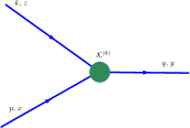
Figure 1: We here show schematically a 3-valent event marked by a $\mathcal{K}^{(0)}$ that symbolizes a boundary term conventionally located at value $s_{0}$ of the affine parameter $s$. The boundary term enforces (deformed) momentum conservation at the event.

The formalism introduced in Ref. principle allows the description of such an event in terms of the law of on-shellness, which for the $\kappa$-momentum space is (1), and the law of composition of momenta, which for the $\kappa$-momentum space is (2). This is done by introducing the action principle

$$\begin{array}[]{lll}\mathcal{S}&=&\int_{-\infty}^{s_{0}}ds\left(z^{\mu}\dot{k}_{\mu}+\mathcal{N}_{k}[\mathcal{C}_{k}-m_{k}^{2}]\right)+\int_{-\infty}^{s_{0}}ds\left({x}^{\mu}\dot{p}_{\mu}+\mathcal{N}_{p}[\mathcal{C}_{p}-m_{p}^{2}]\right)+\int_{s_{0}}^{+\infty}ds\left(y^{\mu}\dot{q}_{\mu}+\mathcal{N}_{q}[\mathcal{C}_{q}-m_{q}^{2}]\right)-\xi_{(0)}^{\mu}\mathcal{K}_{\ \mu}^{(0)}\,.\end{array}$$ (3)

Here the Lagrange multipliers $\mathcal{N}_{k}$,$\mathcal{N}_{p}$,$\mathcal{N}_{q}$ enforce in standard way the on-shellness of particles. The most innovative part of the formalization introduced in Ref. principle is the presence of boundary terms at endpoints of worldlines, enforcing momentum conservation. In the case of (3), describing the single interaction in Fig.1, there is only one such boundary term, and the momentum-conservation-enforcing $\mathcal{K}_{\ \mu}^{(0)}$ takes the form

$$\begin{split}{\cal K}^{(0)}_{\ \mu}&=(k\oplus p)_{\mu}-q_{\mu}\ .\end{split}$$ (4)

Relative spacetime locality is an inevitable feature of descriptions of events governed by curvature of momentum space of the type illustrated by our example (3). To see this we vary the action (3) keeping the momenta fixed at $s=\pm\infty$, as prescribed in Ref. principle , and we find the equations of motion

$$\dot{k}_{\mu}=0\leavevmode\nobreak\ ,\leavevmode\nobreak\ \leavevmode\nobreak\ \dot{p}_{\mu}=0\leavevmode\nobreak\ ,\leavevmode\nobreak\ \leavevmode\nobreak\ \dot{q}_{\mu}=0\leavevmode\nobreak\ ,\leavevmode\nobreak\ \leavevmode\nobreak\$$ (5)

$$\mathcal{C}_{k}=m_{k}^{2}\leavevmode\nobreak\ ,\leavevmode\nobreak\ \leavevmode\nobreak\ \mathcal{C}_{p}=m_{p}^{2}\leavevmode\nobreak\ ,\leavevmode\nobreak\ \leavevmode\nobreak\ \mathcal{C}_{q}=m_{q}^{2}\leavevmode\nobreak\ ,\leavevmode\nobreak\ \leavevmode\nobreak\$$ (6)

$$\mathcal{K}_{\mu}^{(0)}=0,$$ (7)

$$\dot{z}^{\mu}=\mathcal{N}_{k}\frac{\partial\mathcal{C}_{k}}{\partial k_{\mu}}\leavevmode\nobreak\ ,\leavevmode\nobreak\ \leavevmode\nobreak\ \leavevmode\nobreak\ \dot{x}^{\mu}=\mathcal{N}_{p}\frac{\partial\mathcal{C}_{p}}{\partial p_{\mu}}\leavevmode\nobreak\ ,\leavevmode\nobreak\ \leavevmode\nobreak\ \leavevmode\nobreak\ \dot{y}^{\mu}=\mathcal{N}_{q}\frac{\partial\mathcal{C}_{q}}{\partial q_{\mu}}\,,$$ (8)

and the boundary conditions at the endpoints of the 3 semi-infinite worldlines

$$z^{\mu}(s_{0})=\xi^{\nu}_{(0)}\frac{\partial\mathcal{K}_{\nu}^{(0)}}{\partial k_{\mu}}\leavevmode\nobreak\ ,\leavevmode\nobreak\ \leavevmode\nobreak\ \leavevmode\nobreak\ x^{\mu}(s_{0})=\xi^{\nu}_{(0)}\frac{\partial\mathcal{K}_{\nu}^{(0)}}{\partial p_{\mu}}\leavevmode\nobreak\ ,\leavevmode\nobreak\ \leavevmode\nobreak\ \leavevmode\nobreak\ y^{\mu}(s_{0})=-\xi^{\nu}_{(0)}\frac{\partial\mathcal{K}_{\nu}^{(0)}}{\partial q_{\mu}}\ .$$ (9)

The relative locality is codified in the fact that for configurations such that $\xi_{(0)}^{\mu}\neq 0$ the boundary conditions (9) impose that the endpoints of the worldlines do not coincide, since in general

$$\frac{\partial\mathcal{K}_{\nu}^{(0)}}{\partial k_{\mu}}\neq\frac{\partial\mathcal{K}_{\nu}^{(0)}}{\partial p_{\mu}}\neq-\frac{\partial\mathcal{K}_{\nu}^{(0)}}{\partial q_{\mu}}\ ,$$ (10)

so that in the coordinatization of the (in that case, distant) observer the interaction appears to be non-local. However, as shown in Fig.2, for observers such that the same configuration is described with $\xi_{(0)}^{\mu}=0$ the endpoints of the worldlines must coincide and be located in the origin of the observer ($x^{\mu}(s_{0})=y^{\mu}(s_{0})=z^{\mu}(s_{0})=0$).

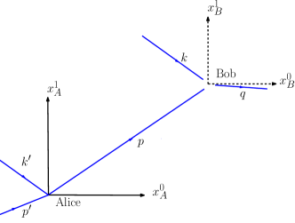
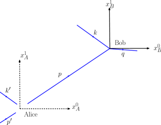
Figure 2: We here give a schematic description of a process composed of two causally-connected events. The event at Alice could be the absorption of a photon by an atom and the event at Bob could be another absorption of a photon by the same atom. The implications of relative locality are visualized by describing Alice’s perspective on the process in the left panel and the perspective of Bob (distant from Alice and in relative rest with respect to Alice) in the right panel. According to Alice’s description the first absorption event (which occurs in Alice’s origin of the reference frame) is local, but Alice’s inferences about the second absorption event (which occurs at Bob, far away from Alice) would characterize it as non-local. Bob has a relativistically specular viewpoint: Bob’s description of the second absorption event (which occurs in Bob’s origin of the reference frame) is local but Bob’s inferences about the first absorption event (which occurs at Alice, far away from Bob) would characterize it as non-local. This is how a pair of causally-connected distant local events gets described in presence of relative locality.

And it is important to notice that taking as starting point of the analysis some observer Alice for whom $\xi_{(0)[A]}^{\mu}\neq 0$, i.e. an observer distant from the interaction who sees the interaction as non-local, one can obtain from Alice an observer Bob for whom $\xi_{(0)[B]}^{\mu}=0$ if the transformation from Alice to Bob for endpoints of coordinates has the form

$$\begin{split}z^{\mu}_{B}(s_{0})&=z^{\mu}_{A}(s_{0})-\xi_{A}^{\nu}\frac{\partial\mathcal{K}_{\nu}^{(0)}}{\partial k_{\mu}}\ ,\\ x^{\mu}_{B}(s_{0})&=x^{\mu}_{A}(s_{0})-\xi_{A}^{\nu}\frac{\partial\mathcal{K}_{\nu}^{(0)}}{\partial p_{\mu}}\ ,\\ y^{\mu}_{B}(s_{0})&=y^{\mu}_{A}(s_{0})+\xi_{A}^{\nu}\frac{\partial\mathcal{K}_{\nu}^{(0)}}{\partial q_{\mu}}\ .\end{split}$$ (11)

Such a property for the endpoints is produced of course, for the choice $b^{\nu}=\xi_{A}^{\nu}$, by the corresponding prescription for the translation transformations:

$$\begin{split}x^{\mu}_{B}(s)&=x^{\mu}_{A}(s)-b^{\nu}\frac{\partial\mathcal{K}_{\nu}}{\partial p_{\mu}}=x^{\mu}_{A}(s)+b^{\nu}\{(k\oplus p)_{\nu},x^{\mu}(s)\}\ ,\\ z^{\mu}_{B}(s)&=z^{\mu}_{A}(s)-b^{\nu}\frac{\partial\mathcal{K}_{\nu}}{\partial k_{\mu}}=z^{\mu}_{A}(s)+b^{\nu}\{(k\oplus p)_{\nu},z^{\mu}(s)\}\ ,\\ y^{\mu}_{B}(s)&=y^{\mu}_{A}(s)+b^{\nu}\frac{\partial\mathcal{K}_{\nu}}{\partial q_{\mu}}=y^{\mu}_{A}(s)+b^{\nu}\{q_{\nu},y^{\mu}(s)\}\ ,\\ \xi_{B}^{\mu}&=\xi_{A}^{\mu}-b^{\mu}\ .\end{split}$$ (12)

where it is understood that $\{x^{\mu},p_{\nu}\}=\delta^{\mu}_{\nu}$, $\{z^{\mu},k_{\nu}\}=\delta^{\mu}_{\nu}$, $\{y^{\mu},q_{\nu}\}=\delta^{\mu}_{\nu}$. This also shows that in this framework one can enforce the “principle of relative locality” principle that all interactions are local according to nearby observers (observers such that the interaction occurs in the origin of their reference frame).

III Cause and effect, with relative locality

Technically our goal is to work within the framework briefly reviewed in the previous section (and described in more detail and generality in Refs.principle ; anatomy ), specifically assuming the laws (1) and (2) for the $\kappa$-momentum space, and show that the concerns for causality reported in Ref.linq and the concerns for momentum conservation reported in Ref.andrb do not apply once the principle of relative locality is enforced. We start with the causality issue and before considering specifically the concerns discussed in Ref.linq we devote this section to an aside on the relationship between cause and effect in our framework. We just intend to show that relative locality, though weaker than ordinary absolute locality, is strong enough to ensure the objectivity of the causal link between a cause and its effect. An example of situation where this is not a priori obvious with relative locality is the one in Fig.3, where we illustrate schematically two causal links: a pair of causally-connected events is shown in red and another pair of causally-connected events is shown in blue, but there is no causal connection (in spite of the coincidence of the events ${\cal K}^{(0)}$ and ${\cal K}^{(1)}$) between events where blue lines cross and events where red lines cross. An example of situation of the type shown in Fig.3 is the one of two atoms getting both coincidently excited by photon absorption, then both propagating freely and ultimately both getting de-excited by emitting a photon each.

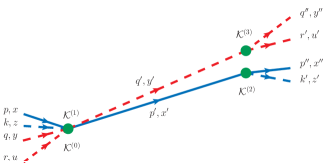
Figure 3: We here show schematically two causal links: a pair of causally-connected events is shown in red and another pair of causally-connected events is shown in blue, but there is no causal connection (in spite of the coincidence of the events ${\cal K}^{(0)}$ and ${\cal K}^{(1)}$) between events where blue lines cross and events where red lines cross. We analyze this situation with the simplifying assumption that some of the particles involved (those described by dashed lines) have energies small enough that the Planck-scale effects here of interest can be safely neglected.

A problem might arise when (as suggested in Fig.3) events on two different causal links happen to be rather close in spacetime: because of relative locality observers distant from such near-coincident (but uncorrelated) events might get a sufficiently distorted picture of the events that the causal links could get confused. We will arrange for a particularly insightful such situation by the end of this section. And ultimately we shall find that no confusion about causal links arises if information on the different events is gathered by nearby observers. Specifically for the situation in Fig.3 it will be necessary to rely on at least two observers: an observer Alice near events $\mathcal{K}_{\ \mu}^{(0)}$ and $\mathcal{K}_{\ \mu}^{(1)}$ and an observer Bob near events $\mathcal{K}_{\ \mu}^{(2)}$ and $\mathcal{K}_{\ \mu}^{(3)}$.

We shall do this analysis in detail but making some simplifying assumptions about the energies of the particles involved. For the particles described by dashed lines in Fig.3 we assume that they are “soft” anatomy , i.e. their energies $E$ are small enough that terms of order $\ell E^{2}$ are negligible in comparison to all other energy scales that we shall instead take into account. The particles described by solid lines in Fig.3 are instead “hard”, meaning that for them $\ell$ corrections must be taken into account. We also adopt the simplification that all particles are ultrarelativistic, i.e. for massive particles the mass can be neglected.

The action describing the situation in Fig.3 within the relative-locality curved-momentum-space framework proposed in Ref. principle is

$$\begin{array}[]{lll}\mathcal{S}&=&\displaystyle\int_{-\infty}^{s_{1}}ds\left(z^{\mu}\dot{k}_{\mu}+\mathcal{N}_{k}\mathcal{C}_{k}^{(0)}\right)+\int_{-\infty}^{s_{1}}ds\left({x}^{\mu}\dot{p}_{\mu}+\mathcal{N}_{p}(\mathcal{C}_{p}-m_{p}^{2})\right)+\int_{-\infty}^{s_{0}}ds\left(y^{\mu}\dot{q}_{\mu}+\mathcal{N}_{q}(\mathcal{C}_{q}^{(0)}-m^{2}_{q})\right)+\\ &&\displaystyle\int_{-\infty}^{s_{0}}ds\left({u}^{\mu}\dot{r}_{\mu}+\mathcal{N}_{r}\mathcal{C}_{r}^{(0)}\right)+\int_{s_{1}}^{s_{2}}ds\left({x^{\prime}}^{\mu}\dot{p}^{\prime}_{\mu}+\mathcal{N}_{p^{\prime}}(\mathcal{C}_{p^{\prime}}-m_{p^{\prime}}^{2})\right)+\int_{s_{0}}^{s_{3}}ds\left(y^{\prime\mu}\dot{q}^{\prime}_{\mu}+\mathcal{N}_{q^{\prime}}(\mathcal{C}_{q^{\prime}}^{(0)}-m_{q^{\prime}}^{2})\right)+\\ &&\displaystyle\int_{s_{3}}^{+\infty}ds\left(y^{\prime\prime\mu}\dot{q}^{\prime\prime}_{\mu}+\mathcal{N}_{q^{\prime\prime}}(\mathcal{C}_{q^{\prime\prime}}^{(0)}-m^{2}_{q^{\prime\prime}})\right)+\int_{s_{3}}^{+\infty}ds\left({u^{\prime}}^{\mu}\dot{r}^{\prime}_{\mu}+\mathcal{N}_{r^{\prime}}\mathcal{C}_{r^{\prime}}^{(0)}\right)+\int_{s_{2}}^{+\infty}ds\left(x^{\prime\prime\mu}\dot{p}^{\prime\prime}_{\mu}+\mathcal{N}_{p^{\prime\prime}}(\mathcal{C}_{p^{\prime\prime}}-m_{p^{\prime\prime}}^{2})\right)+\\ &&\displaystyle\int_{s_{2}}^{+\infty}ds\left(z^{\prime\mu}\dot{k^{\prime}}_{\mu}+\mathcal{N}_{k^{\prime}}\mathcal{C}_{k^{\prime}}^{(0)}\right)-\xi_{(0)}^{\mu}\mathcal{K}_{\ \mu}^{(0)}-\xi_{(1)}^{\mu}\mathcal{K}_{\ \mu}^{(1)}-\xi_{(2)}^{\mu}\mathcal{K}_{\ \mu}^{(2)}-\xi_{(3)}^{\mu}\mathcal{K}_{\ \mu}^{(3)}\ ,\end{array}$$ (13)

where the ${\cal K}^{(i)}_{\ \mu}$ appearing in the boundary terms enforce the relevant conservation laws

$$\begin{split}{\cal K}^{(0)}_{\ \mu}&=(r\oplus q)_{\mu}-q^{\prime}_{\mu}\ ,\\ {\cal K}^{(1)}_{\ \mu}&=(k\oplus p)_{\mu}-p^{\prime}_{\mu}\ ,\\ {\cal K}^{(2)}_{\ \mu}&=p^{\prime}_{\mu}-(k^{\prime}\oplus p^{\prime\prime})_{\mu}\ ,\\ {\cal K}^{(3)}_{\ \mu}&=q^{\prime}_{\mu}-(r^{\prime}\oplus q^{\prime\prime})_{\mu}\ .\end{split}$$ (14)

Several aspects of (13) are worth emphasizing. First we notice that the action in (13) is just the sum of two independent pieces, one for each (two-event-)chain of causally-connected events. For soft particles we codified the on-shellness in terms of $\mathcal{C}^{(0)}_{p}=p_{0}^{2}-p_{1}^{2}$, while for hard particles we have $\mathcal{C}_{p}\equiv p_{0}^{2}-p_{1}^{2}-\ell p_{0}p_{1}^{2}$, appropriate for the $\kappa$-momentum case. For conceptually clarity massive particles in (13) are identifiable indeed because we write a mass term for them, even though, as announced, we shall assume throughout this section that all particles are ultrarelativistic. Also note that the action (13) is not specialized to the case which will be here of interest from the causality perspective, which is the case of coincidence of the two events ${\cal K}^{(0)}$ and ${\cal K}^{(1)}$: we shall enforce that feature later by essentially focusing on cases such that $\xi^{\mu}_{(0)}=\xi^{\mu}_{(1)}$.

By varying the action (13), one obtains the following equations of motion

$$\dot{p}_{\mu}=0\leavevmode\nobreak\ ,\leavevmode\nobreak\ \leavevmode\nobreak\ \dot{q}_{\mu}=0\leavevmode\nobreak\ ,\leavevmode\nobreak\ \leavevmode\nobreak\ \dot{k}_{\mu}=0\leavevmode\nobreak\ ,\leavevmode\nobreak\ \leavevmode\nobreak\ \dot{r}_{\mu}=0\leavevmode\nobreak\ ,\leavevmode\nobreak\ \leavevmode\nobreak\ \dot{p}^{\prime}_{\mu}=0\leavevmode\nobreak\ ,\leavevmode\nobreak\ \leavevmode\nobreak\ \dot{q}^{\prime}_{\mu}=0\leavevmode\nobreak\ ,\leavevmode\nobreak\ \leavevmode\nobreak\ \dot{p}^{\prime\prime}_{\mu}=0\leavevmode\nobreak\ ,\leavevmode\nobreak\ \leavevmode\nobreak\ \dot{q}^{\prime\prime}_{\mu}=0\leavevmode\nobreak\ ,\leavevmode\nobreak\ \leavevmode\nobreak\ \dot{k}^{\prime}_{\mu}=0\leavevmode\nobreak\ ,\leavevmode\nobreak\ \leavevmode\nobreak\ \dot{r}^{\prime}_{\mu}=0\ ,$$

$$\mathcal{C}_{p}=m_{p}^{2}\leavevmode\nobreak\ ,\leavevmode\nobreak\ \leavevmode\nobreak\ \mathcal{C}_{q}^{(0)}=m^{2}_{q}\leavevmode\nobreak\ ,\leavevmode\nobreak\ \leavevmode\nobreak\ \mathcal{C}_{k}^{(0)}=0\leavevmode\nobreak\ ,\leavevmode\nobreak\ \leavevmode\nobreak\ \mathcal{C}_{r}^{(0)}=0\leavevmode\nobreak\ ,\leavevmode\nobreak\ \leavevmode\nobreak\ \mathcal{C}_{p^{\prime}}=m_{p^{\prime}}^{2}\leavevmode\nobreak\ ,\leavevmode\nobreak\ \leavevmode\nobreak\ \mathcal{C}_{q^{\prime}}^{(0)}=m_{q^{\prime}}^{2}\leavevmode\nobreak\ ,\leavevmode\nobreak\ \leavevmode\nobreak\ \mathcal{C}_{p^{\prime\prime}}=m_{p^{\prime\prime}}^{2}\leavevmode\nobreak\ ,\leavevmode\nobreak\ \leavevmode\nobreak\ \mathcal{C}_{q^{\prime\prime}}^{(0)}=m^{2}_{q^{\prime\prime}}\leavevmode\nobreak\ ,\leavevmode\nobreak\ \leavevmode\nobreak\ \mathcal{C}_{k^{\prime}}^{(0)}=0\leavevmode\nobreak\ ,\leavevmode\nobreak\ \leavevmode\nobreak\ \mathcal{C}_{r^{\prime}}^{(0)}=0\ ,$$

$${\cal K}^{(0)}_{\mu}=0\leavevmode\nobreak\ ,\leavevmode\nobreak\ \leavevmode\nobreak\ \leavevmode\nobreak\ {\cal K}^{(1)}_{\mu}=0\leavevmode\nobreak\ ,\leavevmode\nobreak\ \leavevmode\nobreak\ \leavevmode\nobreak\ {\cal K}^{(2)}_{\mu}=0\leavevmode\nobreak\ ,\leavevmode\nobreak\ \leavevmode\nobreak\ \leavevmode\nobreak\ {\cal K}^{(3)}_{\mu}=0\ ,$$

$$\dot{x}^{\mu}=\mathcal{N}_{p}\frac{\partial\mathcal{C}_{p}}{\partial p_{\mu}}\leavevmode\nobreak\ ,\leavevmode\nobreak\ \leavevmode\nobreak\ \leavevmode\nobreak\ \dot{y}^{\mu}=\mathcal{N}_{q}\frac{\partial\mathcal{C}_{q}^{(0)}}{\partial q_{\mu}}\leavevmode\nobreak\ ,\leavevmode\nobreak\ \leavevmode\nobreak\ \leavevmode\nobreak\ \dot{z}^{\mu}=\mathcal{N}_{k}\frac{\partial\mathcal{C}_{k}^{(0)}}{\partial k_{\mu}}\leavevmode\nobreak\ ,\leavevmode\nobreak\ \leavevmode\nobreak\ \leavevmode\nobreak\ \dot{u}^{\mu}=\mathcal{N}_{r}\frac{\partial\mathcal{C}_{r}^{(0)}}{\partial r_{\mu}}\leavevmode\nobreak\ ,\leavevmode\nobreak\ \leavevmode\nobreak\ \leavevmode\nobreak\$$

$$\dot{x}^{\prime\mu}=\mathcal{N}_{p^{\prime}}\frac{\partial\mathcal{C}_{p^{\prime}}}{\partial p^{\prime}_{\mu}}\leavevmode\nobreak\ ,\leavevmode\nobreak\ \leavevmode\nobreak\ \leavevmode\nobreak\ {\dot{y}}^{\prime\mu}=\mathcal{N}_{q^{\prime}}\frac{\partial\mathcal{C}_{q^{\prime}}^{(0)}}{\partial q_{\mu}^{\prime}}\leavevmode\nobreak\ ,\leavevmode\nobreak\ \leavevmode\nobreak\ \leavevmode\nobreak\ \dot{x}^{\prime\prime\mu}=\mathcal{N}_{p^{\prime\prime}}\frac{\partial\mathcal{C}_{p^{\prime\prime}}}{\partial p^{\prime\prime}_{\mu}}\leavevmode\nobreak\ ,\leavevmode\nobreak\ \leavevmode\nobreak\ \leavevmode\nobreak\ \dot{y}^{\prime\prime\mu}=\mathcal{N}_{q^{\prime\prime}}\frac{\partial\mathcal{C}_{q^{\prime\prime}}^{(0)}}{\partial q^{\prime\prime}_{\mu}}\leavevmode\nobreak\ ,\leavevmode\nobreak\ \leavevmode\nobreak\ \leavevmode\nobreak\ \dot{z}^{\prime\mu}=\mathcal{N}_{k^{\prime}}\frac{\partial\mathcal{C}_{k^{\prime}}^{(0)}}{\partial k^{\prime}_{\mu}}\leavevmode\nobreak\ ,\leavevmode\nobreak\ \leavevmode\nobreak\ \leavevmode\nobreak\ \dot{u}^{\prime\mu}=\mathcal{N}_{r^{\prime}}\frac{\partial\mathcal{C}_{r^{\prime}}^{(0)}}{\partial r^{\prime}_{\mu}}\leavevmode\nobreak\ ,\leavevmode\nobreak\ \leavevmode\nobreak\ \leavevmode\nobreak\$$

and the boundary conditions for the endpoints of the worldlines

$$x^{\mu}(s_{1})=\xi^{\nu}_{(1)}\frac{\partial\mathcal{K}^{(1)}_{\nu}}{\partial p_{\mu}}\leavevmode\nobreak\ ,\leavevmode\nobreak\ \leavevmode\nobreak\ \leavevmode\nobreak\ z^{\mu}(s_{1})=\xi^{\nu}_{(1)}\frac{\partial\mathcal{K}^{(1)}_{\nu}}{\partial k_{\mu}}\leavevmode\nobreak\ ,\leavevmode\nobreak\ \leavevmode\nobreak\ \leavevmode\nobreak\ y^{\mu}(s_{0})=\xi^{\nu}_{(0)}\frac{\partial\mathcal{K}^{(0)}_{\nu}}{\partial q_{\mu}}\leavevmode\nobreak\ ,\leavevmode\nobreak\ \leavevmode\nobreak\ \leavevmode\nobreak\ u^{\mu}(s_{0})=\xi^{\nu}_{(0)}\frac{\partial\mathcal{K}^{(0)}_{\nu}}{\partial r_{\mu}}\leavevmode\nobreak\ ,\leavevmode\nobreak\ \leavevmode\nobreak\ \leavevmode\nobreak\ x^{\prime\mu}(s_{1})=-\xi^{\nu}_{(1)}\frac{\partial\mathcal{K}^{(1)}_{\nu}}{\partial p^{\prime}_{\mu}}\leavevmode\nobreak\ ,\leavevmode\nobreak\ \leavevmode\nobreak\ \leavevmode\nobreak\$$

$$\qquad x^{\prime\mu}(s_{2})=\xi^{\nu}_{(2)}\frac{\partial\mathcal{K}^{(2)}_{\nu}}{\partial p^{\prime}_{\mu}}\leavevmode\nobreak\ ,\leavevmode\nobreak\ \leavevmode\nobreak\ \leavevmode\nobreak\ y^{\prime\mu}(s_{0})=-\xi^{\nu}_{(0)}\frac{\partial\mathcal{K}^{(0)}_{\nu}}{\partial q^{\prime}_{\mu}}\leavevmode\nobreak\ ,\leavevmode\nobreak\ \leavevmode\nobreak\ \leavevmode\nobreak\ y^{\prime\mu}(s_{3})=\xi^{\nu}_{(3)}\frac{\partial\mathcal{K}^{(3)}_{\nu}}{\partial q^{\prime}_{\mu}}\leavevmode\nobreak\ ,\leavevmode\nobreak\ \leavevmode\nobreak\ \leavevmode\nobreak\ x^{\prime\prime\mu}(s_{2})=-\xi^{\nu}_{(2)}\frac{\partial\mathcal{K}^{(2)}_{\nu}}{\partial p^{\prime\prime}_{\mu}}\leavevmode\nobreak\ ,\leavevmode\nobreak\ \leavevmode\nobreak\ \leavevmode\nobreak\ z^{\prime\mu}(s_{2})=-\xi^{\nu}_{(2)}\frac{\partial\mathcal{K}^{(2)}_{\nu}}{\partial k^{\prime}_{\mu}}\leavevmode\nobreak\ ,\leavevmode\nobreak\ \leavevmode\nobreak\ \leavevmode\nobreak\$$

$$y^{\prime\prime\mu}(s_{3})=-\xi^{\nu}_{(3)}\frac{\partial\mathcal{K}^{(3)}_{\nu}}{\partial q^{\prime\prime}_{\mu}}\leavevmode\nobreak\ ,\leavevmode\nobreak\ \leavevmode\nobreak\ \leavevmode\nobreak\ u^{\prime\mu}(s_{3})=-\xi^{\nu}_{(3)}\frac{\partial\mathcal{K}^{(3)}_{\nu}}{\partial r^{\prime}_{\mu}}\leavevmode\nobreak\ \ .$$

It is easy to check that the above equations of motion and boundary conditions are invariant under the following translation transformations:

$$\begin{split}x^{\mu}_{B}&=x^{\mu}_{A}+b^{\nu}\{(k\oplus p)_{\nu},x^{\mu}\}\ ,\\ z^{\mu}_{B}&=z^{\mu}_{A}+b^{\nu}\{(k\oplus p)_{\nu},z^{\mu}\}\ ,\\ y^{\mu}_{B}&=y^{\mu}_{A}+b^{\nu}\{(r\oplus q)_{\nu},y^{\mu}\}\ ,\\ u^{\mu}_{B}&=u^{\mu}+b^{\nu}\{(r\oplus q)_{\nu},u^{\mu}\}\ ,\\ {x^{\prime}}^{\mu}_{B}&={x^{\prime}}_{A}^{\mu}+b^{\nu}\{p^{\prime}_{\nu},{x^{\prime}}^{\mu}\}\ ,\\ {y^{\prime}}_{B}^{\mu}&={y^{\prime}}_{A}^{\mu}+b^{\nu}\{q^{\prime}_{\nu},{y^{\prime}}^{\mu}\}\ ,\\ {x^{\prime\prime}}^{\mu}_{B}&=x^{\prime\prime\mu}_{A}+b^{\nu}\{(k^{\prime}\oplus p^{\prime\prime})_{\nu},x^{\prime\prime\mu}\}\ ,\\ {z^{\prime}}^{\mu}_{B}&=z^{\prime\mu}_{A}+b^{\nu}\{k^{\prime}\oplus p^{\prime\prime})_{\nu},z^{\prime\mu}\}\ ,\\ {y^{\prime\prime}}^{\mu}_{B}&=y^{\prime\prime\mu}_{A}+b^{\nu}\{(r^{\prime}\oplus q^{\prime\prime})_{\nu},y^{\prime\prime\mu}\}\ ,\\ {u^{\prime}}^{\mu}_{B}&=u^{\prime\mu}_{A}+b^{\nu}\{(r^{\prime}\oplus q^{\prime\prime})_{\nu},u^{\prime\mu}\}\ ,\end{split}$$ (15)

where $b^{\mu}$ are the translation parameters and it is understood that $\{z^{\mu},k_{\nu}\}=\delta^{\mu}_{\nu}$, $\{x^{\mu},p_{\nu}\}=\delta^{\mu}_{\nu}$, $\{y^{\mu},q_{\nu}\}=\delta^{\mu}_{\nu}$, $\{u^{\mu},r_{\nu}\}=\delta^{\mu}_{\nu}$, $\{z^{\prime\mu},k^{\prime}_{\nu}\}=\delta^{\mu}_{\nu}$, $\{x^{\prime\mu},p^{\prime}_{\nu}\}=\delta^{\mu}_{\nu}$, $\{y^{\prime\mu},q^{\prime}_{\nu}\}=\delta^{\mu}_{\nu}$, $\{u^{\prime\mu},r^{\prime}_{\nu}\}=\delta^{\mu}_{\nu}$, $\{x^{\prime\prime\mu},p^{\prime\prime}_{\nu}\}=\delta^{\mu}_{\nu}$, $\{y^{\prime\prime\mu},q^{\prime\prime}_{\nu}\}=\delta^{\mu}_{\nu}$.

Because of relative locality we evidently need here two observers Alice and Bob chosen so that the questions here of interest can be investigated in terms of the locality of interactions near them. As announced we focus on the case in which the interactions ${\cal K}^{(0)}$ and ${\cal K}^{(1)}$ are coincident, and we take as Alice an observer for whom these two interactions occur in the origin of her reference frame. This in particular allows us to restrict our attention to cases with $x^{\prime\mu}_{A}(s_{1})=y^{\prime\mu}_{A}(s_{0})=0$. We take the other observer, Bob, at rest with respect to Alice and such that the event ${\cal K}^{(3)}$ occurs in the origin of Bob’s reference frame, so that $y^{\prime\mu}_{B}(s_{3})=0$. Since in the $\kappa$-momentum case the physical speed of ultrarelativistic particles depends on their energy anatomy the interaction ${\cal K}^{(2)}$ cannot be coincident with the interaction ${\cal K}^{(3)}$ (since ${\cal K}^{(0)}$ and ${\cal K}^{(3)}$ exchange a soft particle whereas ${\cal K}^{(1)}$ and ${\cal K}^{(2)}$ exchange a hard particle one must take into account the difference in physical speed between the hard and the soft exchanged particle). But this dependence on energy of the physical speed of ultrarelativistic particles is anyway a small $\ell$-suppressed effect, so we can focus on a situation where ${\cal K}^{(2)}$ and ${\cal K}^{(3)}$ are nearly coincident, and we study that situation assuming ${\cal K}^{(2)}$ occurs in spatial origin of Bob’s reference frame (but at time different from ${\cal K}^{(3)}$). This allows us to specify $x^{\prime 1}_{B}(s_{2})=0$. Also note that as long as the distance of ${\cal K}^{(2)}$ from the spacetime origin of Bob’s reference frame is an $\ell$-suppressed feature Bob’s description of the locality (or lack thereof) of the interaction ${\cal K}^{(2)}$ is automatically immune from relative-locality effects at leading order in $\ell$, which is the order at which we are working.

Equipped with this choice of observers and these simplifying assumptions about the relevant events, we can quickly advance with our analysis of causal links from the relative-locality perspective. We start by noticing that from the equations of motion it follows that both for Alice and Bob

$$\frac{\dot{x}^{\prime 1}}{\dot{x}^{\prime 0}}=1-\ell p^{\prime}_{1}\,,\qquad\frac{\dot{y}^{\prime 1}}{\dot{y}^{\prime 0}}=1\,.$$ (16)

This implies that according to Alice (for whom the events ${\cal K}^{(0)}$ and ${\cal K}^{(1)}$ occur in the origin of the reference frame) the worldlines of the two exchanged particles are

$$\begin{split}{x^{\prime}}_{A}^{1}&=(1-\ell p^{\prime}_{1}){x^{\prime}}_{A}^{0}\ ,\\ {y^{\prime}}_{A}^{1}&={y^{\prime}}_{A}^{0}\ .\end{split}$$ (17)

A key aspect of the analysis we are reporting in this section is establishing how these two worldlines are described by the distant observer Bob. On the basis of (15) one concludes that the relevant translation transformation is undeformed:

$$\begin{split}{x^{\prime}}_{B}^{\mu}(s)&={x^{\prime}}_{A}^{\mu}(s)+b^{\nu}\{p^{\prime}_{\nu},x^{\prime\mu}\}={x^{\prime}}_{A}^{\mu}(s)-b^{\mu}\ ,\\ {y^{\prime}}_{B}^{\mu}(s)&={y^{\prime}}_{A}^{\mu}(s)+b^{\nu}\{q^{\prime}_{\nu},y^{\prime\mu}\}={y^{\prime}}_{A}^{\mu}(s)-b^{\mu}\ .\end{split}$$ (18)

So the worldlines in Bob’s coordinatization must have the form

$$\begin{split}x^{\prime 1}_{B}&=(1-\ell p^{\prime}_{1})x^{\prime 0}_{B}-b^{1}+b^{0}-b^{0}\ell p^{\prime}_{1}\,,\\ y^{\prime 1}_{B}&=y^{\prime 0}_{B}-b^{1}+b^{0}\,.\end{split}$$ (19)

Since we have specified for Bob that ${\cal K}^{(3)}$ occurs in the origin of his reference frame, $y^{\prime\mu}_{B}(s_{3})=0$, we must have that $b^{0}=b^{1}$. And then finally we establish that the event ${\cal K}^{(2)}$, occurring in the spatial origin of Bob’s reference frame, $x^{1}_{B}(s_{2})=0$, is timed by Bob at

$$x^{\prime 0}_{B}(s_{2})=b^{1}\ell p^{\prime}_{1}\ .$$ (20)

In particular for positive $\ell$ one has that according to Bob ${\cal K}^{(2)}$ occurs before ${\cal K}^{(3)}$ in his spatial origin, with a time difference between them given by $\Delta t=b^{1}\ell p^{\prime}_{1}$.

This was just preparatory material for the point we most care about in this section, which concerns possible paradoxes for causality and their clarification. For that we need to look at how Alice describes the two events distant from her, ${\cal K}^{(2)}$ and ${\cal K}^{(3)}$. ${\cal K}^{(3)}$ is an interaction involving only soft particles so nothing noteworthy can arise from looking at ${\cal K}^{(3)}$, but ${\cal K}^{(2)}$ involves hard particles and therefore the inferences about ${\cal K}^{(2)}$ by observer Alice, who is distant from ${\cal K}^{(2)}$, will give a description of ${\cal K}^{(2)}$ as an apparently non-local interaction. This is the main implication of relative locality, and we can see that it does give rise to a combined description of ${\cal K}^{(2)}$ and ${\cal K}^{(3)}$ that at first may appear puzzling from the causality perspective. We show this by noting down the values of coordinates of particles involved in ${\cal K}^{(2)}$ and ${\cal K}^{(3)}$ according to Alice. For the particles with coordinates $y^{\prime\prime\mu}$ and $u^{\prime\mu}$ on the basis of (15) one finds that the translation is completely undeformed, and since $y^{\prime\prime\mu}_{B}(s_{3})=u^{\prime\mu}_{B}(s_{3})=0$ one has that

$$y^{\prime\prime\mu}_{A}(s_{3})=u^{\prime\mu}_{A}(s_{3})=\xi_{(3)A}^{\mu}=b^{1}\ .$$

For the particles involved in the hard vertex ${\cal K}^{(2)}$, with coordinates $x^{\prime\prime\mu}$ and $z^{\prime\mu}$, on the basis of (15) one finds that the translation is deformed, and starting from the fact that $x^{\prime\prime 0}_{B}=b^{1}\ell p^{\prime}_{1}$, $x^{\prime\prime 1}_{B}=0$, $z^{\prime 0}_{B}=b^{1}\ell p^{\prime}_{1}$, $z^{\prime 1}_{B}=0$ one arrives at finding that

$$\begin{split}x^{\prime\prime 0}_{A}(s_{2})&=b^{1}+b^{1}\ell p^{\prime}_{1}\ ,\\ x^{\prime\prime 1}_{A}(s_{2})&=b^{1}-b^{1}\ell k^{\prime}_{1}\ \approx b^{1},\\ z^{\prime 0}_{A}(s_{2})&=b^{1}+b^{1}\ell p^{\prime}_{1}-b^{1}\ell p^{\prime\prime}_{1}\ ,\\ z^{\prime 1}_{A}(s_{2})&=b^{1}\ .\end{split}$$ (21)

As shown in Fig.4 the most striking situation from the viewpoint of causality arises when $p^{\prime}_{1}\simeq p^{\prime\prime}_{1}$, in which case according to Alice $z^{\prime 0}_{A}(s_{2})=z^{\prime 1}_{A}(s_{2})=b^{1}$, which means that the particle with coordinates $z^{\prime\mu}$, who actually interacts at ${\cal K}^{(2)}$, in the coordinatization by distant observer Alice appears to come out of the interaction ${\cal K}^{(3)}$. This is an example of the sort of apparent paradoxes for causality that can be encountered with relative locality: they all concern the description of events by distant observers. Of course, there is no true paradox since a known consequence of relative locality is that inferences about distant events are misleading. Indeed, as also shown in Fig.4, Bob’s description of the interactions ${\cal K}^{(2)}$ and ${\cal K}^{(3)}$ (which are near Bob) is completely unproblematic. However, in turn, Bob’s inferences about the events ${\cal K}^{(0)}$ and ${\cal K}^{(1)}$ (which are distant from Bob) are affected by peculiar relative-locality features, as also shown in Fig.4. In looking at Fig.4 readers should also keep in mind that for that figure we magnified effects in order to render them visible: actually all noteworthy features in Fig.4 are Planck-scale suppressed, and would amount to time intervals no greater than $10^{-19}s$ for Earth experiments (over distances of, say, $10^{6}m$) involving particles with currently accessible energies (no greater than, say, $1TeV$).

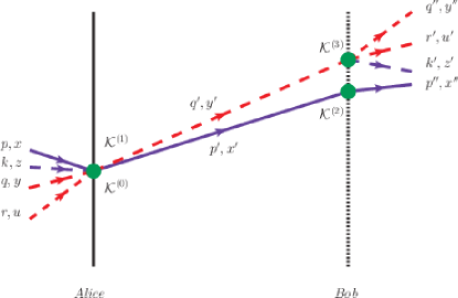
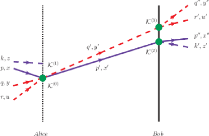
Figure 4: The two causally-connected pairs of events considered in this section can lead to a striking picture of distant inferences (because of relative locality) when $p^{\prime}_{1}\simeq p^{\prime\prime}_{1}$. In that case the particle with coordinates $z^{\prime\mu}$, who actually interacts at ${\cal K}^{(2)}$, in the coordinatization by distant observer Alice (top panel) appears to come out of the interaction ${\cal K}^{(3)}$. In turn, as we show in the bottom panel of the figure, Bob’s inferences about the events ${\cal K}^{(0)}$ and ${\cal K}^{(1)}$ (which are distant from Bob) are affected by peculiar relative-locality features.

IV Causal Loops

The observations on relative locality reported in the previous two sections illustrate how misleading the characterization of events and chains of events can be, if not based on how each event is seen by a nearby observer. For chains of events this imposes that the analysis be based on more than one observer: at least one observer for each interaction in the chain.

Equipped with this understanding we now progress to the next level in testing causality: we consider the possibility of a “causal loop”, i.e. a chain of events that form a loop in such a way that causality would be violated.

The starting point for being concerned about these causal loops is the analysis reported in Ref.linq , which considered a loop diagram of the type here shown in Fig.5. Ref.linq works on a curved momentum space, but without enforcing relative locality, and finds that a causal loop of the type here shown in Fig.5 could be possible. Our objective is to show that such causal loops are excluded if one enforces relative locality. In light of the observations reported in the previous two sections we shall of course need to study the loop diagram in Fig.5 on the basis of the findings of two observers, one near the first interaction and one near the second interaction (whereas the analysis of Ref.linq only considered the perspective of one observer, in which case the principle of relativity of spacetime locality cannot be enforced or investigated).

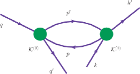
Figure 5: We here show schematically a pair of events causally connected by the exchange of two particles arranged in such a way that one would have a causal loop. Such causal loops are allowed, if one assumes curvature of momentum space without enforcing (DSR-)relativistic covariance and the associated relativity of spacetime locality.

We stress that here, just as in Ref.linq , we are working at the level of classical mechanics, so the loop diagram in Fig.5 involves all particles on-shell and merely keeps track of the causal links among different events, assigning worldlines exiting/entering each event (one should not confuse such loop diagrams with the different notion arising in Feynman’s perturbative approach to quantum field theory).

We start by writing down an action of the type already considered in the previous two sections, which gives the description of the loop diagram in Fig.5 within the relative-locality curved-momentum-space formalism proposed in Ref.principle . We shall see that our action does reproduce the equations of motion and the boundary conditions which were at the basis of the analysis reported in Ref.linq . This action giving the diagram in Fig. 5 is

$$\begin{array}[]{lll}\mathcal{S}&=&\displaystyle\int_{-\infty}^{s_{0}}ds\left(y^{\mu}\dot{q}_{\mu}+\mathcal{N}_{q}(\mathcal{C}_{q}-m^{2}_{q})\right)+\int_{s_{0}}^{+\infty}ds\left(y^{\prime\mu}\dot{q}_{\mu}^{\prime}+\mathcal{N}_{q^{\prime}}(\mathcal{C}_{q^{\prime}}-m^{2}_{q^{\prime}})\right)+\int_{-\infty}^{s_{1}}ds\left(z^{\mu}\dot{k}_{\mu}+\mathcal{N}_{k}(\mathcal{C}_{k}-m^{2}_{k})\right)+\\ &&\displaystyle+\int_{s_{1}}^{+\infty}ds\left(z^{\prime\mu}\dot{k}^{\prime}_{\mu}+\mathcal{N}_{k^{\prime}}(\mathcal{C}_{k^{\prime}}-m^{2}_{k^{\prime}})\right)+\int_{s_{0}}^{s_{1}}ds\left(x^{\prime\mu}\dot{p}^{\prime}_{\mu}+\mathcal{N}_{p^{\prime}}(\mathcal{C}_{p^{\prime}}-m^{2}_{p^{\prime}})\right)+\int_{s_{1}}^{s_{0}}ds\left(x^{\mu}\dot{p}_{\mu}+\mathcal{N}_{p}(\mathcal{C}_{p}-m^{2}_{p})\right)+\\ &&\displaystyle-\xi_{(0)}^{\mu}\mathcal{K}_{\mu}^{(0)}-\xi_{(1)}^{\mu}\mathcal{K}_{\mu}^{(1)}\ ,\end{array}$$ (22)

where $\mathcal{K}_{\mu}^{(0)}=\left[(q\oplus p)\oplus(\ominus(p^{\prime}\oplus q^{\prime}))\right]_{\mu}$ and $\mathcal{K}_{\mu}^{(1)}=\left[(p^{\prime}\oplus k)\oplus(\ominus(k^{\prime}\oplus p))\right]_{\mu}$. It is important for us to stress, since this is the key ingredient for seeking a violation of causality, that the last integral, which stands for the free propagation of the particle which is travelling back in time, has inverted integration extrema.

By varying this action we obtain equations of motion

$$\dot{p}_{\mu}=0\ ,\qquad\dot{p}^{\prime}_{\mu}=0\ ,\qquad\dot{q}_{\mu}=0\ ,\qquad\dot{q}^{\prime}_{\mu}=0\ ,\qquad\dot{k}_{\mu}=0\ ,\qquad\dot{k}^{\prime}_{\mu}=0\ ,$$ (23a)

$$\mathcal{C}_{p}=m^{2}_{p}\ ,\qquad\mathcal{C}_{p^{\prime}}=m^{2}_{p^{\prime}}\ ,\qquad\mathcal{C}_{q}=m^{2}_{q}\ ,\qquad\mathcal{C}_{q^{\prime}}=m^{2}_{q^{\prime}}\ ,\qquad\mathcal{C}_{k^{\prime}}=m^{2}_{k^{\prime}}\ ,\qquad\mathcal{C}_{k}=m^{2}_{k}\ ,$$ (23b)

$$\dot{x}^{\mu}(s)=\mathcal{N}_{p}\frac{\partial\mathcal{C}_{p}}{\partial p_{\mu}}\ ,\qquad\dot{x}^{\prime\mu}(s)=\mathcal{N}_{p^{\prime}}\frac{\partial\mathcal{C}_{p^{\prime}}}{\partial p^{\prime}_{\mu}}\ ,\qquad\dot{y}^{\mu}(s)=\mathcal{N}_{q}\frac{\partial\mathcal{C}_{q}}{\partial q_{\mu}}\ ,$$ (23c)

$$\dot{y}^{\prime\mu}(s)=\mathcal{N}_{q^{\prime}}\frac{\partial\mathcal{C}_{q^{\prime}}}{\partial q^{\prime}_{\mu}}\ ,\qquad\dot{z}^{\mu}(s)=\mathcal{N}_{k}\frac{\partial\mathcal{C}_{k}}{\partial k_{\mu}}\ ,\qquad\dot{z}^{\prime\mu}(s)=\mathcal{N}_{k^{\prime}}\frac{\partial\mathcal{C}_{k^{\prime}}}{\partial k^{\prime}_{\mu}}\ ,$$ (23d)

$$\mathcal{K}_{\mu}^{(0)}=0\ ,\qquad\mathcal{K}_{\mu}^{(1)}=0\ ,$$ (23e)

and boundary terms

$$y^{\mu}(s_{0})=\xi_{(0)}^{\nu}\frac{\partial\mathcal{K}_{\nu}^{(0)}}{\partial q_{\mu}}\ ,\qquad y^{\prime\mu}(s_{0})=-\xi_{(0)}^{\nu}\frac{\partial\mathcal{K}_{\nu}^{(0)}}{\partial q^{\prime}_{\mu}}\ ,\qquad z^{\prime\mu}(s_{1})=-\xi_{(1)}^{\nu}\frac{\partial\mathcal{K}_{\nu}^{(1)}}{\partial k^{\prime}_{\mu}}\ ,\qquad z^{\mu}(s_{1})=\xi_{(1)}^{\nu}\frac{\partial\mathcal{K}_{\nu}^{(1)}}{\partial k_{\mu}}\ ,$$ (24a)

$$x^{\mu}(s_{0})=\xi_{(0)}^{\nu}\frac{\partial\mathcal{K}_{\nu}^{(0)}}{\partial p_{\mu}}\ ,\qquad x^{\mu}(s_{1})=-\xi_{(1)}^{\nu}\frac{\partial\mathcal{K}_{\nu}^{(1)}}{\partial p_{\mu}}\ ,\qquad x^{\prime\mu}(s_{0})=-\xi_{(0)}^{\nu}\frac{\partial\mathcal{K}_{\nu}^{(0)}}{\partial p^{\prime}_{\mu}}\ ,\qquad x^{\prime\mu}(s_{1})=\xi_{(1)}^{\nu}\frac{\partial\mathcal{K}_{\nu}^{(1)}}{\partial p^{\prime}_{\mu}}\ ,$$ (24b)

which indeed reproduce the ones used in the analysis reported in Ref.linq .

IV.1 Aside on the absence of causal loops in Special Relativity

We find it useful to start by first considering the $\ell\rightarrow 0$ limit of the problem of interest in this section: the causal loop in Special Relativity (i.e. with Minkowskian geometry of momentum space). This allows us to assume temporarily that the on-shellness is governed by $\mathcal{C}^{(0)}=p_{0}^{2}-p_{1}^{2}$ and that therefore the following relationship holds

$$\dot{x}^{\mu}(s)=\left(\dot{x}^{\nu}\dot{x}_{\nu}\right)^{\frac{1}{2}}\frac{p^{\mu}}{m_{p}}\ .$$ (25)

We take advantage of some simplification of analysis, without loosing any of the conceptual ingredients here of interest, by focusing on $\dot{x}_{\mu}\dot{x}^{\mu}>0,\ \dot{x}^{0}>0;\ p^{2}=m_{p}^{2}>0,\ p^{0}\geq m_{p}>0$, i.e. our particles travel along timelike worldlines. We have that the proper time of a particle is given by

$$d\tau=\left(\dot{x}^{\mu}\dot{x}_{\mu}\right)^{\frac{1}{2}}ds=\dot{x}^{0}\sqrt{1-\left(\frac{\dot{x}^{1}}{\dot{x}^{0}}\right)^{2}}ds=\dot{x}^{0}\sqrt{1-\left(\frac{p^{1}}{p^{0}}\right)^{2}}ds=\dot{x}^{0}\gamma_{p}^{-1}ds\ ,$$ (26)

where $\gamma_{p}$ is the usual Lorentz factor and in the third equality we used (25).

Going back to the diagram in Fig.5 we have that for the particle with phase-space coordinates $(p^{\prime},x^{\prime})$, whose worldline is exchanged between the interaction $\mathcal{K}^{(0)}$ and the interaction $\mathcal{K}^{(1)}$ (and therefore travels from $x^{\prime\mu}(s_{0})$ to $x^{\prime\mu}(s_{1})$) the following chain of equalities holds

$$\begin{array}[]{lll}x^{\prime\mu}(s_{1})-x^{\prime\mu}(s_{0})&=&\displaystyle\int_{s_{0}}^{s_{1}}ds\,\frac{dx^{\prime\mu}}{ds}=\int_{s_{0}}^{s_{1}}ds\left(\dot{x}^{\prime\nu}\dot{x}^{\prime}_{\nu}\right)^{\frac{1}{2}}\frac{p^{\prime\mu}}{m_{p^{\prime}}}=\\ &=&\displaystyle\int_{\tau^{\prime}(s_{0})}^{\tau^{\prime}(s_{1})}d\tau^{\prime}\frac{p^{\prime\mu}}{m_{p^{\prime}}}=\Delta\tau^{\prime}u^{\prime\mu}\ ,\end{array}$$ (27)

with $\displaystyle u^{\prime\mu}=\frac{p^{\prime\mu}}{m_{p^{\prime}}}$  .

Similarly, for the other particle exchanged between $\mathcal{K}^{(0)}$ and $\mathcal{K}^{(1)}$, the one with phase-space coordinates $(p,x)$, one has that

$$\begin{array}[]{lll}x^{\mu}(s_{0})-x^{\mu}(s_{1})&=&\displaystyle\int_{s_{1}}^{s_{0}}ds\,\frac{dx^{\mu}}{ds}=\int_{s_{1}}^{s_{0}}ds\left(\dot{x}^{\nu}\dot{x}_{\nu}\right)^{\frac{1}{2}}\frac{p^{\mu}}{m_{p}}=\\ &=&\displaystyle\int_{\tau(s_{1})}^{\tau(s_{0})}d\tau\frac{p^{\mu}}{m_{p}}=\Delta\tau\ u^{\mu}\ .\end{array}$$ (28)

Since in this subsection we are working in the $\ell\rightarrow 0$ limit we have that $\mathcal{K}_{\mu}^{(0)}=q_{\mu}+p_{\mu}-p^{\prime}_{\mu}-q^{\prime}_{\mu}$ and $\mathcal{K}_{\mu}^{(1)}=p^{\prime}_{\mu}+k_{\mu}-k^{\prime}_{\mu}-p_{\mu}$ , in which case it is easy to see that our boundary conditions simply enforce

$$\xi_{(0)}^{\mu}=x^{\prime\mu}(s_{0})\leavevmode\nobreak\ ,\leavevmode\nobreak\ \leavevmode\nobreak\ \leavevmode\nobreak\ \xi_{(0)}^{\mu}=x^{\mu}(s_{0})\leavevmode\nobreak\ ,\leavevmode\nobreak\ \leavevmode\nobreak\ \leavevmode\nobreak\ \xi_{(1)}^{\mu}=x^{\prime\mu}(s_{1})\leavevmode\nobreak\ ,\leavevmode\nobreak\ \leavevmode\nobreak\ \leavevmode\nobreak\ \xi_{(1)}^{\mu}=x^{\mu}(s_{1})\leavevmode\nobreak\ .$$ (29)

So evidently

$$\xi_{(1)}^{\mu}-\xi_{(0)}^{\mu}=x^{\prime\mu}(s_{1})-x^{\prime\mu}(s_{0})=\Delta\tau^{\prime}u^{\prime\mu}\ ,$$ (30)

$$\xi_{(0)}^{\mu}-\xi_{(1)}^{\mu}=x^{\mu}(s_{0})-x^{\mu}(s_{1})=\Delta\tau\ u^{\mu}\ ,$$ (31)

and

$$\Delta\tau\ u^{\mu}+\Delta\tau^{\prime}u^{\prime\mu}=0\ .$$ (32)

Since the relevant proper-time intervals are positive and the zero components of the four-velocities are positive this requirement can never be satisfied: as well known causal loops are forbidden in Special Relativity.

Another way to see that causal loops are forbidden in Special Relativity can be based on deriving the relationship between the relevant proper-time intervals and the interaction coordinates $\xi_{(0)}^{\mu}$, $\xi_{(1)}^{\mu}$. One easily finds that

$$\Delta\tau=\int_{s_{1}}^{s_{0}}ds\ \dot{x}^{0}\gamma_{p}^{-1}=\gamma_{p}^{-1}\left(x^{0}(s_{0})-x^{0}(s_{1})\right)=\gamma_{p}^{-1}\left(\xi_{(0)}^{0}-\xi_{(1)}^{0}\right)\ ,$$ (33)

$$\Delta\tau^{\prime}=\int_{s_{0}}^{s_{1}}ds\ \dot{x}^{\prime 0}\gamma_{p^{\prime}}^{-1}=\gamma_{p^{\prime}}^{-1}\left(x^{\prime 0}(s_{1})-x^{\prime 0}(s_{0})\right)=\gamma_{p^{\prime}}^{-1}\left(\xi_{(1)}^{0}-\xi_{(0)}^{0}\right)\ .$$ (34)

So again the fact that $\Delta\tau\geq 0$ and $\Delta\tau^{\prime}\geq 0$ excludes the causal loop, since on the basis of (33)-(34) this would require $\xi_{(0)}=\xi_{(1)}$: by construction $\left(\xi_{(1)}-\xi_{(0)}\right)_{\mu}\left(\xi_{(1)}-\xi_{(0)}\right)^{\mu}\geq 0$ (the interval between the two interactions is timelike or null) and then $\xi_{(0)}^{0}=\xi_{(1)}^{0}$ implies $\xi_{(0)}^{\mu}=\xi_{(1)}^{\mu}$, i.e. the loop can only collapse into a single event (no causality issue, not a causal loop).

IV.2 Causal loop with curved momentum space

Our next step is to introduce leading-order-in-$\ell$ corrections, but without enforcing the principle of relative locality. Such setups in general do allow causal loops, as we shall now show (in agreement with what was already claimed in Ref.linq ). What changes with respect to the special-relativistic case of the previous subsection is that (for the $\kappa$-momentum case, which we chose as illustrative example) the on-shellness is governed by $\mathcal{C}_{p}=p_{0}^{2}-p_{1}^{2}-\ell p_{0}p_{1}^{2}$ while conservation laws at first order take the form

$$\mathcal{K}_{\ 0}^{(0)}=q_{0}+p_{0}-q^{\prime}_{0}-p^{\prime}_{0}\ ,$$ (35a)

$$\mathcal{K}_{\ 1}^{(0)}=q_{1}+p_{1}-q^{\prime}_{1}-p^{\prime}_{1}-\ell\left[q_{0}p_{1}-(q_{0}+p_{0}-q^{\prime}_{0}-p^{\prime}_{0})p^{\prime}_{1}-(q_{0}+p_{0}-q^{\prime}_{0})q^{\prime}_{1}\right]\ ,$$ (35b)

$$\mathcal{K}_{\ 0}^{(1)}=p^{\prime}_{0}+k_{0}-p_{0}-k^{\prime}_{0}\ ,$$ (35c)

$$\mathcal{K}_{\ 1}^{(1)}=p^{\prime}_{1}+k_{1}-p_{1}-k^{\prime}_{1}-\ell\left[p^{\prime}_{0}k_{1}-(p^{\prime}_{0}+k_{0}-p_{0}-k^{\prime}_{0})k^{\prime}_{1}-(p^{\prime}_{0}+k_{0}-p_{0})p_{1}\right]\ .$$ (35d)

Also the equations of motion are $\ell$-deformed, as shown in (23c)-(23d), and for example one has that

$$\dot{x}^{\mu}(s)=\mathcal{N}_{p}\left[2p^{\mu}-\ell\left(\delta^{\mu}_{0}p_{1}^{2}+\delta^{\mu}_{1}2p_{0}p_{1}\right)\right]\ .$$ (36)

This still allows one to write a relationship analogous to (25) from the previous subsection,

$$\dot{x}^{\mu}(s)=\left(\dot{x}^{\nu}\dot{x}_{\nu}\right)^{\frac{1}{2}}u^{\mu}\ ,$$ (37)

but with

$$u^{\mu}=\frac{p^{\mu}}{m_{p}}-\frac{\ell}{2m_{p}}\left(-2p^{\mu}\frac{p_{0}p_{1}^{2}}{m_{p}^{2}}+\delta_{0}^{\mu}p_{1}^{2}+\delta^{\mu}_{1}2p_{0}p_{1}\right)\ .$$

Analogously, for $x^{\prime\mu}$ one has that

$$\dot{x}^{\prime\mu}(s)=\left(\dot{x}^{\prime\nu}\dot{x}^{\prime}_{\nu}\right)^{\frac{1}{2}}u^{\prime\mu}\ ,$$ (38)

with

$$u^{\prime\mu}=\frac{p^{\prime\mu}}{m_{p^{\prime}}}-\frac{\ell}{2m_{p^{\prime}}}\left(-2p^{\prime\mu}\frac{p^{\prime}_{0}p_{1}^{\prime 2}}{m_{p^{\prime}}^{2}}+\delta_{0}^{\mu}p_{1}^{\prime 2}+\delta^{\mu}_{1}2p^{\prime}_{0}p^{\prime}_{1}\right)\ .$$

In close analogy with (27) and (28) one easily finds that

$$x^{\prime\mu}(s_{1})-x^{\prime\mu}(s_{0})=\Delta\tau^{\prime}u^{\prime\mu},$$ (39)

$$x^{\mu}(s_{0})-x^{\mu}(s_{1})=\Delta\tau\ u^{\mu}\leavevmode\nobreak\ ,$$ (40)

and from (24b) it follows that

$$\xi_{(0)}^{\nu}=-x^{\prime\mu}(s_{0})\left(\frac{\partial\mathcal{K}_{\nu}^{(0)}}{\partial p^{\prime}_{\mu}}\right)^{-1}=x^{\mu}(s_{0})\left(\frac{\partial\mathcal{K}_{\nu}^{(0)}}{\partial p_{\mu}}\right)^{-1}\ ,$$ (41)

$$\xi_{(1)}^{\nu}=x^{\prime\mu}(s_{1})\left(\frac{\partial\mathcal{K}_{\nu}^{(1)}}{\partial p^{\prime}_{\mu}}\right)^{-1}=-x^{\mu}(s_{1})\left(\frac{\partial\mathcal{K}_{\nu}^{(1)}}{\partial p_{\mu}}\right)^{-1}\ .$$ (42)

Combining (41) with (40) one finds that

$$-x^{\prime\mu}(s_{0})\left(\frac{\partial\mathcal{K}_{\nu}^{(0)}}{\partial p^{\prime}_{\mu}}\right)^{-1}\frac{\partial\mathcal{K}_{\nu}^{(0)}}{\partial p_{\rho}}=x^{\rho}(s_{0})=x^{\rho}(s_{1})+\Delta\tau u_{p}^{\rho}\ ,$$ (43)

while combining (42) with (39) one finds that

$$x^{\rho}(s_{1})=-x^{\prime\mu}(s_{1})\left(\frac{\partial\mathcal{K}_{\nu}^{(1)}}{\partial p^{\prime}_{\mu}}\right)^{-1}\frac{\partial\mathcal{K}_{\nu}^{(1)}}{\partial p_{\rho}}=-(x^{\prime\mu}(s_{0})+\Delta\tau^{\prime}u^{\prime\mu})\left(\frac{\partial\mathcal{K}_{\nu}^{(1)}}{\partial p^{\prime}_{\mu}}\right)^{-1}\frac{\partial\mathcal{K}_{\nu}^{(1)}}{\partial p_{\rho}}\ .$$ (44)

Finally, combining (44) with (43), we obtain the same condition given in linq ,

$$\left[\frac{\partial\mathcal{K}_{\nu}^{(1)}}{\partial p_{\rho}}\left(\frac{\partial\mathcal{K}_{\nu}^{(1)}}{\partial p^{\prime}_{\mu}}\right)^{-1}-\frac{\partial\mathcal{K}_{\nu}^{(0)}}{\partial p_{\rho}}\left(\frac{\partial\mathcal{K}_{\nu}^{(0)}}{\partial p^{\prime}_{\mu}}\right)^{-1}\right]x^{\prime\mu}(s_{0})=-\frac{\partial\mathcal{K}_{\nu}^{(1)}}{\partial p_{\rho}}\left(\frac{\partial\mathcal{K}_{\nu}^{(1)}}{\partial p^{\prime}_{\mu}}\right)^{-1}\Delta\tau^{\prime}u^{\prime\mu}+\Delta\tau u^{\rho}\ ,$$ (45)

which takes the following form upon expanding $\mathcal{K}_{\nu}^{(0)}$ and $\mathcal{K}_{\nu}^{(1)}$ to leading order in $\ell$:

$$\ell\left[\delta_{1}^{\rho}\left(k^{\prime}_{0}-q_{0}\right)+\delta_{0}^{\rho}\left(q^{\prime}_{1}-k_{1}\right)\right]x^{\prime 1}(s_{0})=\Delta\tau u^{\rho}+\Delta\tau^{\prime}\left[u^{\prime\rho}+u^{\prime 1}\ell\left(\delta_{0}^{\rho}k_{1}-\delta_{1}^{\rho}k^{\prime}_{0}\right)\right]\ .$$ (46)

This (46) is what replaces (32) when the causal loop is analyzed on a curved momentum space without enforcing relative locality.

Notice that this (46), when its left-hand side does not vanish, can have solutions with positive $\Delta\tau$ and $\Delta\tau^{\prime}$ and positive zero components of the four-velocities, which was not possible with (32). This means that contrary to the special-relativistic case (Minkowski momentum space) causal loops are possible on a curved momentum space, at least if one does not enforce relative locality.

We also note down some equalities that follow from (46) and therefore must hold for the causal loop to be allowed

$$\Delta\tau=-\Delta\tau^{\prime}\frac{u^{\prime 0}}{u^{0}}+\ell x^{\prime 1}(s_{0})\left(\frac{q^{\prime}_{1}-k_{1}}{u^{0}}\right)-\ell\Delta\tau^{\prime}\left(\frac{u^{\prime 1}k_{1}}{u^{0}}\right)\ ,$$ (47)

$$\ell x^{\prime 1}(s_{0})=\Delta\tau^{\prime}\frac{u^{1}u^{\prime 0}-u^{0}u^{\prime 1}+\ell u^{\prime 1}(k_{1}u^{1}+k^{\prime}_{0}u^{0})}{u^{0}(q_{0}-k^{\prime}_{0})+u^{1}(q^{\prime}_{1}-k_{1})}$$ (48)

and we note that in order for (47) to have acceptable solutions one must have that

$$x^{\prime 1}(s_{0})>\frac{\Delta\tau^{\prime}(u^{\prime 0}+\ell u^{\prime 1}k_{1})}{\ell|q^{\prime}_{1}-k_{1}|}\ .$$ (49)

This is in good agreement with the results of Ref. linq , but we find useful to add some observations to those reported in Ref. linq . A first point to notice is that Eq. (49) appears to suggest that $x^{\prime 1}$ should take peculiarly large values, as in some of the estimates given in Ref. linq , since $x^{\prime 1}$ has magnitude set by a formula with the small scale $\ell$ in the denominator. If one could conclude that only cases with ultralarge $x^{\prime 1}$ allowed such a causal loop, then the violations of causality would be to some extent less concerning (if confined to a range of values of $x^{\prime 1}$ large enough to fall outside our observational window). However, it is easy to see that (49) does not really impose any restriction on the size of $x^{\prime 1}$: one will have that typically $x^{\prime 1}$ is much larger than $\Delta\tau^{\prime}$ but there are causal loops for any value of $x^{\prime 1}$ (under the condition of taking suitable values of $\Delta\tau^{\prime}$ and $\Delta\tau$). So when momentum space is curved and one does not enforce the relativity of spacetime locality the violations of causality are rather pervasive.

There is also a technical point that deserves some comments and is related to this pervasiveness of the violations of causality: it might appear to be surprising that within a perturbative expansion, assuming small $\ell$, one arrives at a formula like (49), with $\ell$ in the denominator. This is however not so surprising considering the role of $x^{\prime 1}$ in this sort of analysis. The main clarification comes from observing that in the unperturbed theory (the $\ell=0$ theory, i.e. special relativity) $x^{\prime 1}$ is completely undetermined: as shown in the previous subsection the only causal loops allowed in special relativity are those that collapse (no violation of causality) and such collapsed causal loops are allowed for any however large or however small value of $x^{\prime 1}$. As stressed above this fact that $x^{\prime 1}$ can take any value is preserved by the $\ell$ corrections. The apparently surprising factor of $1/\ell$ only appears in a relationship between $x^{\prime 1}$ and $\Delta\tau^{\prime}$. If $x^{\prime 1}$ and $\Delta\tau^{\prime}$ both had some fixed finite value in the $\ell=0$ theory than at finite small $\ell$ their values should change by very little. But since in the $\ell=0$ theory $x^{\prime 1}$ is unconstrained (in particular it could take any however large value) and its value is not linked in any way to the value $\Delta\tau^{\prime}$, then it is not surprising that the $\ell$ corrections take the form shown for example in (49).

IV.3 Causal loop analysis in 3+1 dimensions

So far we examined the 1+1-dimensional case, but it is rather evident that the features we discussed in the previous subsection are not an artifact of that dimensional reduction. Nonetheless it is worth pausing briefly in this subsection for verifying that indeed those features are still present in $3+1$ dimensions. In this case the on-shellness is governed by $\mathcal{C}_{p}=p_{0}^{2}-\vec{p}^{2}-\ell p_{0}\vec{p}^{2}$ while conservation laws at first order take the form

$$\mathcal{K}_{\ 0}^{(0)}=q_{0}+p_{0}-q^{\prime}_{0}-p^{\prime}_{0}\ ,$$ (50a)

$$\mathcal{K}_{\ i}^{(0)}=q_{i}+p_{i}-q^{\prime}_{i}-p^{\prime}_{i}-\ell\delta_{i}^{j}\left[q_{0}p_{j}-(q_{0}+p_{0}-q^{\prime}_{0}-p^{\prime}_{0})p^{\prime}_{j}-(q_{0}+p_{0}-q^{\prime}_{0})q^{\prime}_{j}\right]\ ,$$ (50b)

$$\mathcal{K}_{\ 0}^{(1)}=p^{\prime}_{0}+k_{0}-p_{0}-k^{\prime}_{0}\ ,$$ (50c)

$$\mathcal{K}_{\ i}^{(1)}=p^{\prime}_{i}+k_{i}-p_{i}-k^{\prime}_{i}-\ell\delta_{i}^{j}\left[p^{\prime}_{0}k_{j}-(p^{\prime}_{0}+k_{0}-p_{0}-k^{\prime}_{0})k^{\prime}_{j}-(p^{\prime}_{0}+k_{0}-p_{0})p_{j}\right]\ ,$$ (50d)

where $i,j=1,2,3$.

Adopting these expressions, eq.(45), keeping only terms up to first order in $\ell$ in the matrices like $\frac{\partial\mathcal{K}_{\nu}^{(0)}}{\partial p_{\rho}}$ and their products, takes the form

$$\ell\left[\delta_{i}^{\rho}\left(k^{\prime}_{0}-q_{0}\right)+\delta_{0}^{\rho}\left(q^{\prime}_{i}-k_{i}\right)\right]x^{\prime i}(s_{0})=\left[u^{\prime\rho}+u^{\prime i}\ell\left(\delta_{0}^{\rho}k_{i}-\delta_{i}^{\rho}k^{\prime}_{0}\right)\right]\Delta\tau^{\prime}+u^{\rho}\Delta\tau\ ,$$ (51)

or, more clearly, using the energy conservation laws,

$$\begin{split}\ell(q^{\prime}_{1}-k_{1})x^{\prime 1}(s_{0})+\ell(q^{\prime}_{2}-k_{2})x^{\prime 2}(s_{0})+\ell(q^{\prime}_{3}-k_{3})x^{\prime 3}(s_{0})&=(u^{\prime 0}+\ell k_{1}u^{\prime 1}+\ell k_{2}u^{\prime 2}+\ell k_{3}u^{\prime 3})\Delta\tau^{\prime}+u^{0}\Delta\tau,\\ \ell(k_{0}-q^{\prime}_{0})x^{\prime 1}(s_{0})&=(1-\ell k^{\prime}_{0})u^{\prime 1}\Delta\tau^{\prime}+u^{1}\Delta\tau,\\ \ell(k_{0}-q^{\prime}_{0})x^{\prime 2}(s_{0})&=(1-\ell k^{\prime}_{0})u^{\prime 2}\Delta\tau^{\prime}+u^{2}\Delta\tau,\\ \ell(k_{0}-q^{\prime}_{0})x^{\prime 3}(s_{0})&=(1-\ell k^{\prime}_{0})u^{\prime 3}\Delta\tau^{\prime}+u^{3}\Delta\tau.\end{split}$$ (52)

Without really loosing any generality we can analyze the implications of this for an observer orienting her axis of the reference frame so that $p_{i}=0$ and $p^{\prime}_{i}=0$ for $i=2,3$. As a result we also have that $u^{i}=0$ and $u^{\prime i}=0$ for $i=2,3$. For what concerns the other momenta involved in the analysis, $q,\,q^{\prime},\,k,\,k^{\prime}$. this choice of orientation of axis only affects rather mildly the conservation laws:

$$q_{2}=q^{\prime}_{2}-\ell p^{\prime}_{0}q^{\prime}_{2},\qquad q_{3}=q^{\prime}_{3}-\ell p^{\prime}_{0}q^{\prime}_{3},\qquad q^{\prime}_{2}=q_{2}+\ell p^{\prime}_{0}q_{2},\qquad q^{\prime}_{3}=q_{3}+\ell p^{\prime}_{0}q_{3},$$

$$k_{2}=k^{\prime}_{2}+\ell p^{\prime}_{0}k^{\prime}_{2},\qquad k_{3}=k^{\prime}_{3}+\ell p^{\prime}_{0}k^{\prime}_{3},\qquad k^{\prime}_{2}=k_{2}-\ell p^{\prime}_{0}k_{2},\qquad k^{\prime}_{3}=k_{3}-\ell p^{\prime}_{0}k_{3}.$$

Since $u^{i}=0$ and $u^{\prime i}=0$ for $i=2,3$ the last two equations of eq.(52) imply $x^{\prime 2}=0$ and $x^{\prime 3}=0$, which in turn (looking then at the first two equations of eq.(52)) take us back to (47)-(48)

$$\Delta\tau=-\Delta\tau^{\prime}\frac{u^{\prime 0}}{u^{0}}+\ell x^{\prime 1}(s_{0})\left(\frac{q^{\prime}_{1}-k_{1}}{u^{0}}\right)-\ell\Delta\tau^{\prime}\left(\frac{u^{\prime 1}k_{1}}{u^{0}}\right),$$

$$\ell x^{\prime 1}(s_{0})=\Delta\tau^{\prime}\frac{u^{1}u^{\prime 0}-u^{0}u^{\prime 1}+\ell u^{\prime 1}(k_{1}u^{1}+k^{\prime}_{0}u^{0})}{u^{0}(q_{0}-k^{\prime}_{0})+u^{1}(q^{\prime}_{1}-k_{1})}\ .$$

Evidently then all the features discussed for the 1+1-dimensional in the previous subsection are also present in the 3+1-dimensional case.

IV.4 Enforcing Relative Locality

We shall now show that our causal loop is not allowed in theories with curved momentum space if one makes sure that these theories are (DSR-)relativistic, with associated relative locality. This suggests that relative locality is evidently a weaker notion than absolute locality but it is still strong enough to enforce causality.

By definition principle relative locality is such that the locality of events may not be manifest in coordinatizations by distant observers, but for the coordinatizations by observers near an event (ideally at the event) it enforces locality in a way that is no weaker than ordinary locality.

Also notice that the definition of relative locality imposes that translation transformations be formalized in the theory: since one must verify that events are local according to nearby observers (while they may be described as non-local by distant observers) one must use translation transformations in order to ensure that the principle of relative locality principle is enforced. Since our interest is in (DSR-)relativistic theories, of course such translation transformations must be symmetries.

In Ref. anatomy some of us introduced a prescription for having a very powerful implementation of translational invariance in relative-locality theories. One can easily see that the causal loop described in the previous subsections is not compatible with that strong implementation of translational invariance. Evidently then we have that causality is preserved in theories with curved momentum spaces if the strong notion of translational invariance of Ref. anatomy is enforced by postulate.

What we here want to show is that the causal loop of Fig.5 is still forbidden even without enforcing such a strong notion of translational invariance. Causal loops are forbidden even by a minimal notion of translational invariance, the bare minimum needed in order to contemplate relative locality with a DSR-relativistic picture.

Consistently with this objective we ask only for the availability of some translation generator (with possibly complicated momentum dependence) that can enforce the covariance of the equations of motion and the boundary conditions. Let us call our first observer Alice and the second one Bob, purely translated by a parameter $b^{\mu}$ with respect to Alice. For the particles involved inside the loop we have

$$x_{B}^{\mu}(s)=x_{A}^{\mu}(s)-b^{\nu}\mathcal{T}_{\nu}^{\mu}\ ,$$ (53)

$$x_{B}^{\prime\mu}(s)=x_{A}^{\prime\mu}(s)-b^{\nu}\mathcal{T}^{\prime\mu}_{\nu}\ ,$$ (54)

where $\mathcal{T}_{\nu}^{\mu}$ and $\mathcal{T}_{\nu}^{\prime\mu}$ are to be determined through the request of translational invariance.

Combining the first two boundary conditions of (24b) with (53) we obtain

$$-\xi_{B(1)}^{\nu}\frac{\partial\mathcal{K}_{\nu}^{(1)}}{\partial p_{\mu}}=x_{B}^{\mu}(s_{1})=x_{A}^{\mu}(s_{1})-b^{\nu}\mathcal{T}_{\nu}^{\mu}=-\xi_{A(1)}^{\nu}\frac{\partial\mathcal{K}_{\nu}^{(1)}}{\partial p_{\mu}}-b^{\nu}\mathcal{T}_{\nu}^{\mu}\ ,$$ (55)

$$\xi_{B(0)}^{\nu}\frac{\partial\mathcal{K}_{\nu}^{(0)}}{\partial p_{\mu}}=x_{B}^{\mu}(s_{0})=x_{A}^{\mu}(s_{0})-b^{\nu}\mathcal{T}_{\nu}^{\mu}=\xi_{A(0)}^{\nu}\frac{\partial\mathcal{K}_{\nu}^{(0)}}{\partial p_{\mu}}-b^{\nu}\mathcal{T}_{\nu}^{\mu}\leavevmode\nobreak\ .$$ (56)

We find convenient to introduce $\delta\xi_{(i)}^{\nu}\equiv\xi_{B(i)}^{\nu}-\xi_{A(i)}^{\nu}$ and to rewrite equations (55) and (56) as follows

$$b^{\nu}\mathcal{T}_{\nu}^{\mu}=\delta\xi_{(1)}^{\nu}\frac{\partial\mathcal{K}_{\nu}^{(1)}}{\partial p_{\mu}}\ ,$$ (57)

$$b^{\nu}\mathcal{T}_{\nu}^{\mu}=-\delta\xi_{(0)}^{\nu}\frac{\partial\mathcal{K}_{\nu}^{(0)}}{\partial p_{\mu}}\ .$$ (58)

This shows that any form one might speculate about for what concerns translational invariance will still inevitably require enforcing

$$\delta\xi_{(1)}^{\nu}\frac{\partial\mathcal{K}_{\nu}^{(1)}}{\partial p_{\mu}}=-\delta\xi_{(0)}^{\nu}\frac{\partial\mathcal{K}_{\nu}^{(0)}}{\partial p_{\mu}}\ .$$ (59)

Similarly, combining the last two boundary conditions of (24b) with the transformation (54) we obtain

$$-\xi_{B(0)}^{\nu}\frac{\partial\mathcal{K}_{\nu}^{(0)}}{\partial p^{\prime}_{\mu}}=x_{B}^{\prime\mu}(s_{0})=x_{A}^{\prime\mu}(s_{0})-b^{\nu}\mathcal{T}_{\nu}^{\prime\mu}=-\xi_{A(0)}^{\nu}\frac{\partial\mathcal{K}_{\nu}^{(0)}}{\partial p^{\prime}_{\mu}}-b^{\nu}\mathcal{T}_{\nu}^{\prime\mu}\ ,$$ (60)

$$\xi_{B(1)}^{\nu}\frac{\partial\mathcal{K}_{\nu}^{(1)}}{\partial p^{\prime}_{\mu}}=x_{B}^{\prime\mu}(s_{1})=x_{A}^{\prime\mu}(s_{1})-b^{\nu}\mathcal{T}_{\nu}^{\prime\mu}=\xi_{A(1)}^{\nu}\frac{\partial\mathcal{K}_{\nu}^{(1)}}{\partial p^{\prime}_{\mu}}-b^{\nu}\mathcal{T}_{\nu}^{\prime\mu}\ ,$$ (61)

from which it follows that

$$-\delta\xi_{(1)}^{\nu}\frac{\partial\mathcal{K}_{\nu}^{(1)}}{\partial p^{\prime}_{\mu}}=\delta\xi_{(0)}^{\nu}\frac{\partial\mathcal{K}_{\nu}^{(0)}}{\partial p^{\prime}_{\mu}}\ .$$ (62)

The fact that we are insisting only on a minimal requirement of translational invariance is reflected also in the fact that our requirements are more general (weaker) than the ones so far used for translational invariance in previous works on the relative-locality framework. Our requirements (59) and (62) reproduce the ones enforced in Ref. cortes upon opting for boundary terms written in the form $\displaystyle\bigoplus_{i=1}^{i=n}P^{i}_{in}-\bigoplus_{i=1}^{i=m}P^{i}_{out}$, where $P^{i}_{in}$ are the ingoing momenta in a vertex and $P^{i}_{out}$ are the outgoing momenta. And our requirements (59) and (62) reproduce the strong translation transformations enforced in Ref. anatomy , by adopting $\delta\xi_{(1)}^{\nu}=\delta\xi_{(0)}^{\nu}=-b^{\nu}$, i.e., momentum independence of the $\xi^{\mu}$.

Let us next observe that from equation (62) one has that

$$\delta\xi_{(0)}^{\nu}=-\delta\xi_{(1)}^{\sigma}\frac{\partial\mathcal{K}_{\sigma}^{(1)}}{\partial p^{\prime}_{\mu}}\left(\frac{\partial\mathcal{K}_{\nu}^{(0)}}{\partial p^{\prime}_{\mu}}\right)^{-1}\ ,$$ (63)

and using this in equation (59) leads us to

$$\delta\xi_{(1)}^{\sigma}\left[\frac{\partial\mathcal{K}_{\sigma}^{(1)}}{\partial p_{\rho}}-\frac{\partial\mathcal{K}_{\sigma}^{(1)}}{\partial p^{\prime}_{\mu}}\left(\frac{\partial\mathcal{K}_{\nu}^{(0)}}{\partial p^{\prime}_{\mu}}\right)^{-1}\frac{\partial\mathcal{K}_{\nu}^{(0)}}{\partial p_{\rho}}\right]=0\ .$$ (64)

Since $\delta\xi_{(1)}^{\sigma}\neq 0$ (in order for this to be a non-collapsed loop the two observers must be distant) we conclude that

$$\frac{\partial\mathcal{K}_{\nu}^{(1)}}{\partial p_{\rho}}\left(\frac{\partial\mathcal{K}_{\nu}^{(1)}}{\partial p^{\prime}_{\mu}}\right)^{-1}-\frac{\partial\mathcal{K}_{\nu}^{(0)}}{\partial p_{\rho}}\left(\frac{\partial\mathcal{K}_{\nu}^{(0)}}{\partial p^{\prime}_{\mu}}\right)^{-1}=0\ .$$ (65)

This equation (65) plays a pivotal role in our analysis since it shows that an however weak requirement of translational invariance (required for relative locality in a relativistic setup) imposes a restriction on the possible choices of boundary terms. We shall now easily show that once the condition (65) on boundary terms is enforced the causal loop is forbidden. We start by showing that for the boundary terms used in Ref. linq the condition (65) takes the shape of a condition on the momenta involved in the process, specifically, at leading order in $\ell$,

$$\ell\delta_{\mu}^{1}\left[\delta_{1}^{\rho}\left(k^{\prime}_{0}-q_{0}\right)+\delta_{0}^{\rho}\left(q^{\prime}_{1}-k_{1}\right)\right]=0\ ,$$ (66)

which implies that $k^{\prime}_{0}=q_{0}+\mathcal{O}(\ell)$ and $q^{\prime}_{1}=k_{1}+\mathcal{O}(\ell)$. The fact that the causal loop is forbidden can then be seen easily for example by looking back at equation (46), now enforcing (66): one obtains

$$\Delta\tau u^{\rho}+\Delta\tau^{\prime}\left[u^{\prime\rho}+u^{\prime 1}\ell\left(\delta_{0}^{\rho}k_{1}-\delta_{1}^{\rho}k^{\prime}_{0}\right)\right]=0\ .$$ (67)

This excludes the causal loop for just the same reasons that, as observed earlier in this section, the causal loop is excluded in ordinary special relativity: for $\rho=0$ equation (67),

$$\Delta\tau=-\Delta\tau^{\prime}\frac{u^{\prime 0}}{u^{0}}-\ell\Delta\tau^{\prime}\left(\frac{u^{\prime 1}k_{1}}{u^{0}}\right),$$ (68)

does not admit solutions with positive $\Delta\tau$ and $\Delta\tau^{\prime}$ and positive zeroth component of the two 4-velocities. This causal loop is indeed forbidden once a DSR-relativistic description, with associated relative locality, is enforced.

V Möbius diagram and translational invariance

Having shown that the causal loop of Ref.linq is indeed allowed in generic theories on curved momentum spaces, but is forbidden when a DSR-relativistic description, with associated relative spacetime locality, is enforced, we now proceed to the next announced task, which concerns the diagram studied in Ref.andrb as a possible source of violations of global momentum conservation. Ref.andrb considered theories on a curved momentum space, without enforcing relative spacetime locality, and found that in general the diagram shown in our Fig.6 can produce violations of global momentum conservation. These violations take the shape andrb of $k^{\prime}\neq k$, i.e. the momentum incoming into the diagram is not equal to the momentum outgoing from the diagram. Similarly to what we showed in the previous section for a causal loop, we shall find that these violations of global momentum conservation from the diagram in Fig.6 do not occur if one enforces a DSR-relativistic description, with associated relative spacetime locality.

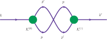
Figure 6: We here show schematically two causally-connected events that form a “Möbius diagram”. The laws of conservation at the two vertices are setup in such a way that the particle outgoing from the first vertex has its momentum appearing on the right-hand side of the composition law and its momentum also appears on the left-hand side of the composition of momenta at the second vertex.

The relative-locality-framework description of the diagram in Fig.6 is obtained through the action

$$\begin{array}[]{lll}\mathcal{S}&=&\displaystyle\int_{-\infty}^{s_{0}}ds\left(z^{\mu}\dot{k}_{\mu}+\mathcal{N}_{k}(\mathcal{C}_{k}-m_{k}^{2})\right)+\int_{s_{1}}^{+\infty}ds\left(z^{\prime\mu}\dot{k}^{\prime}_{\mu}+\mathcal{N}_{k^{\prime}}(\mathcal{C}_{k^{\prime}}-m_{k^{\prime}}^{2})\right)+\\ &+&\displaystyle\int_{s_{0}}^{s_{1}}ds\left(x^{\prime\mu}\dot{p}^{\prime}_{\mu}+\mathcal{N}_{p^{\prime}}(\mathcal{C}_{p^{\prime}}-m_{p^{\prime}}^{2})\right)+\int_{s_{0}}^{s_{1}}ds\left(x^{\mu}\dot{p}_{\mu}+\mathcal{N}_{p}(\mathcal{C}_{p}-m_{p}^{2})\right)+\\ &-&\xi_{(0)}^{\mu}\mathcal{K}_{\mu}^{(0)}-\xi_{(1)}^{\mu}\mathcal{K}_{\mu}^{(1)},\end{array}$$ (69)

with

$$\mathcal{K}_{\ \mu}^{(0)}=\left(k\oplus\left(\ominus\left(p\oplus p^{\prime}\right)\right)\right)_{\mu}\simeq k_{\mu}-p_{\mu}-p^{\prime}_{\mu}+\delta_{\mu}^{1}\ell\left[p_{1}\left(k_{0}-p_{0}-p^{\prime}_{0}\right)+p^{\prime}_{1}\left(k_{0}-p^{\prime}_{0}\right)\right],$$ (70a)

$$\mathcal{K}_{\ \mu}^{(1)}=\left(\left(p^{\prime}\oplus p\right)\oplus\left(\ominus k^{\prime}\right)\right)_{\mu}\simeq p^{\prime}_{\mu}+p_{\mu}-k^{\prime}_{\mu}+\delta_{\mu}^{1}\ell\left[k^{\prime}_{1}\left(p^{\prime}_{0}+p_{0}-k_{0}^{\prime}\right)-p^{\prime}_{0}p_{1}\right].$$ (70b)

From the structure of (70a)-(70b) it is clear why we choose to label the diagram in Fig.6 as a “Möbius diagram”: the laws of conservation at the two vertices use the noncommutativity of the composition law in such a way that the particle outgoing from the first vertex with momentum appearing on the right-hand side of the composition law enters the second vertex with momentum appearing on the left-hand side of the composition law. [Of course, the opposite applies to the other particle exchanged between the vertices]. If one then draws the diagram with the convention that the orientation of pairs of legs entering/exiting a vertex consistently reflects the order in which the momenta are composed, then the only way to draw the diagram makes it resemble a Möbius strip.

Evidently there is no room for such a structure when the momentum space has composition law which is commutative. In particular there is no way to contemplate such a Möbius diagram in special relativity. But on our $\kappa$-momentum space this structure is possible and its implications surely need to be studied.

Consistently with what we reported in the previous sections, our interest is into understanding how the properties of the Möbius diagram are affected if one enforces relative spacetime locality in DSR-relativistic theories on the $\kappa$-momentum space. In particular, we want to show that $k^{\prime}=k$ (no violation of global momentum conservation).

As also already stressed above, relative spacetime locality in a relativistic theory on curved momentum space necessarily requires at least a weak form of translational invariance. This insistence on at least the weakest possible notion of translational invariance led us to find equations (59) and (62) for the causal loop, and, as the interested reader can easily verify, for the case of the Möbius diagram it leads us to the equations

$$\delta\xi^{\nu}_{(0)}\frac{\partial\mathcal{K}^{(0)}_{\nu}}{\partial p_{\mu}}=-\delta\xi^{\nu}_{(1)}\frac{\partial\mathcal{K}^{(1)}_{\nu}}{\partial p_{\mu}},$$ (71a)

$$\delta\xi^{\nu}_{(0)}\frac{\partial\mathcal{K}^{(0)}_{\nu}}{\partial p^{\prime}_{\mu}}=-\delta\xi^{\nu}_{(1)}\frac{\partial\mathcal{K}^{(1)}_{\nu}}{\partial p^{\prime}_{\mu}}.$$ (71b)

These allow us to deduce that

$$\left[\frac{\partial\mathcal{K}^{(1)}_{\sigma}}{\partial p_{\mu}}-\frac{\partial\mathcal{K}^{(1)}_{\sigma}}{\partial p^{\prime}_{\rho}}\left(\frac{\partial\mathcal{K}^{(0)}_{\nu}}{\partial p^{\prime}_{\rho}}\right)^{-1}\frac{\partial\mathcal{K}^{(0)}_{\nu}}{\partial p_{\mu}}\right]=0.$$ (72)

The implications of this equation are best appreciated by exposing explicitly the momentum dependence of the terms appearing in (72):

$$\frac{\partial\mathcal{K}^{(1)}_{\sigma}}{\partial p_{\mu}}=\delta_{\sigma}^{\mu}+\ell\delta_{\sigma}^{1}\left(\delta_{0}^{\mu}k^{\prime}_{1}-\delta_{1}^{\mu}p^{\prime}_{0}\right),$$ (73a)

$$\frac{\partial\mathcal{K}^{(1)}_{\sigma}}{\partial p^{\prime}_{\rho}}=\delta_{\sigma}^{\rho}+\ell\delta_{\sigma}^{1}\delta_{0}^{\rho}\left(k^{\prime}_{1}-p_{1}\right),$$ (73b)

$$\left(\frac{\partial\mathcal{K}^{(0)}_{\nu}}{\partial p^{\prime}_{\rho}}\right)^{-1}=-\delta_{\rho}^{\nu}-\ell\delta_{\rho}^{1}\left[\delta^{\nu}_{1}\left(k_{0}-p^{\prime}_{0}\right)-\delta_{0}^{\nu}\left(p_{1}+p^{\prime}_{1}\right)\right],$$ (73c)

$$\frac{\partial\mathcal{K}^{(0)}_{\nu}}{\partial p_{\mu}}=-\delta^{\mu}_{\nu}-\ell\delta^{\mu}_{0}\delta^{1}_{\nu}p_{1}.$$ (73d)

These allow us to conclude that from (72) it follows that

$$\ell\left[\delta_{1}^{\mu}k_{0}-\delta_{0}^{\mu}\left(p_{1}+p^{\prime}_{1}\right)\right]=0.$$ (74)

Using this result in combination with the conservation laws $\mathcal{K}^{(0)}_{\mu}=0$ and $\mathcal{K}^{(1)}_{\mu}=0$ one can easily establish that

$$p_{\mu}+p^{\prime}_{\mu}=0+\mathcal{O}(\ell)\leavevmode\nobreak\ ,$$ (75)

and one can also rewrite those conservation laws as follows

$$0=k_{\mu}-p_{\mu}-p^{\prime}_{\mu}-\delta_{\mu}^{1}\ell p^{\prime}_{1}p^{\prime}_{0},$$ (76)

$$0=p^{\prime}_{\mu}+p_{\mu}-k^{\prime}_{\mu}-\delta_{\mu}^{1}\ell p^{\prime}_{0}p_{1}\,\,.$$ (77)

Summing these (76) and (77), also using (75), we get to the sought result

$$k_{\mu}=k^{\prime}_{\mu}+\mathcal{O}(\ell^{2})\,\,,$$ (78)

showing that indeed by insisting on a having a DSR-relativistic picture, with associated relative spacetime locality, one finds no global violation of momentum conservation (at least at leading order in $\ell$, which is the level of accuracy we are here pursuing).

VI Combinations of Möbius diagrams and implications for building a quantum theory

In the previous section we reported results suggesting that when theories are (DSR-)relativistic, with the associated relativity of spacetime locality, momentum is globally conserved and there is no violation of causality. It should be noticed that the objective of enforcing relative spacetime locality led us to introduce some restrictions on the choice of boundary terms, particularly for causally-connected interactions. The relevant class of theories has been studied so far only within the confines of classical mechanics, and therefore such prescriptions concerning boundary terms are meaningful and unproblematic (they can indeed be enforced by principle, as a postulate). The quantum version of the theories we here considered is still not known, but if one tries to imagine which shape it might take it seems that enforcing the principle of relative locality in a quantum theory might be very challenging: think in particular of quantum field theories formulated in terms of a generating functional, where all such prescriptions are usually introduced by a single specification of the generating functional. While we do not have anything to report on this point which would address directly the challenges for the construction of such quantum theories, we find it worthy to provide evidence of the fact that combinations of diagrams on curved momentum space might have less anomalous properties, even without enforcing relative locality, than single diagrams.

In an appropriate sense we are attempting to provide first elements in support of a picture which we conjecture ultimately might be somewhat analogous to what happens, for example, in the analysis of the gauge invariance of the first contribution to the matrix element of the Compton scattering $e^{-}+\gamma\rightarrow e^{-}+\gamma$ in standard QED. In fact, in that case there are only two Feynman diagrams that need to be taken into account and the matrix element is given by

$$\mathcal{M}_{fi}=(-ie)^{2}\left(\bar{u}_{p^{\prime}}\not{\epsilon}(q^{\prime})\frac{i}{\not{p}+\not{q}-m}\not{\epsilon}(q)u_{p}+\bar{u}_{p^{\prime}}\not{\epsilon}(q)\frac{i}{\not{p}-\not{q}^{\prime}-m}\not{\epsilon}(q^{\prime})u_{p}\right),$$ (79)

where $p$ and $q$ are the momenta of the electron and the photon respectively in the initial state, $p^{\prime}$ and $q^{\prime}$ are the momenta of the electron and the photon respectively in the final state, $u_{p}$ and $\bar{u}_{p}$ are Dirac spinors and $\epsilon_{\mu}$ is the photon polarization 4-vector. For a free photon described in the Lorentz gauge by a plane wave $A_{\mu}(x)\propto\epsilon_{\mu}(k)e^{\pm ik_{\nu}x^{\nu}}$ the gauge transformation $A_{\mu}^{\Lambda}(x)=A_{\mu}(x)+\partial_{\mu}\Lambda(x)$ with $\Lambda(x)=\tilde{\Lambda}(k)e^{\pm ik_{\nu}x^{\nu}}$ corresponds to a transformation of the polarization 4-vector $\epsilon_{\mu}^{\Lambda}(k)=\epsilon_{\mu}(k)\pm ik_{\mu}\tilde{\Lambda}(k)$. Equipped with these observations one can easily see that the two terms in (79) are not individually gauge invariant, but their combination is gauge invariant.

We are not going to provide conclusive evidence that a similar mechanism is at work for causality and global momentum conservation in theories on curved momentum space (it would be impossible without knowing how to formulate such a quantum theory), but it may be nonetheless interesting that we can find some points of intuitive connection with stories such as that of gauge invariance for Compton scattering.

For definiteness and simplicity we focus on the case of Möbius diagrams. In the previous section we analyzed a Möbius diagram using the choice of boundary terms adopted in Ref. andrb since the appreciation of the presence of a challenge due to Möbius diagrams originated from the study reported in Ref. andrb . In this section we look beyond the realm of considerations offered in Ref. andrb , so we go back to our preferred criterion for the choice of boundary conditions, the one first advocated in Ref.anatomy , which allows us to streamline the derivations. So we consider the Möbius diagram by adopting the following prescription for the boundary terms:

$$\begin{split}\mathcal{K}^{(0)}_{\mu}=k_{\mu}-(p\oplus p^{\prime})_{\mu}\simeq k_{\mu}-p_{\mu}-p^{\prime}_{\mu}+\ell\delta_{\mu}^{1}p_{0}p^{\prime}_{1},\\ \mathcal{K}^{(1)}_{\mu}=(p^{\prime}\oplus p)_{\mu}-k^{\prime}_{\mu}\simeq p^{\prime}_{\mu}+p_{\mu}-k_{\mu}-\ell\delta_{\mu}^{1}p^{\prime}_{0}p_{1}.\end{split}$$ (80)

From the conservation of four-momentum at each vertex $\mathcal{K}^{(0)}_{\mu}=0$, $\mathcal{K}^{(1)}_{\mu}=0$ we get

$$k_{\mu}-k^{\prime}_{\mu}=\ell\delta_{\mu}^{1}(p^{\prime}_{0}p_{1}-p_{0}p^{\prime}_{1})=\ell\delta_{\mu}^{1}(\frac{m_{p}^{2}p^{\prime}_{1}}{2p_{1}}-\frac{m_{p^{\prime}}^{2}p_{1}}{2p^{\prime}_{1}})\equiv\ell\delta_{\mu}^{1}\Delta,$$ (81)

where, since we are considering particles of energy-momentum $\ell^{-1}\gg p_{\mu}\gg m$, from the on-shell relation (1) we expressed the energy of the particles as $p_{0}=\sqrt{p_{1}^{2}+m^{2}}+\frac{\ell p_{1}^{2}}{2}\approx|p_{1}|+\frac{m^{2}}{2|p_{1}|}+\frac{\ell p_{1}^{2}}{2}$.

At this point we must stress that evidently this is not the only way to have a Möbius diagram, since we can interchange the prescription for which particle enters the composition law for the first event on the right side of the composition law (then entering the second event on the left side of the composition law). This alternative possibility (which is the only other possibility allowed within the prescriptions of Ref. anatomy ) is characterized by boundary terms of the form

$$\begin{split}\tilde{\mathcal{K}}^{(0)}_{\mu}=k_{\mu}-(p^{\prime}\oplus p)_{\mu}\simeq k_{\mu}-p^{\prime}_{\mu}-p_{\mu}+\ell\delta_{\mu}^{1}p^{\prime}_{0}p_{1},\\ \tilde{\mathcal{K}}^{(1)}_{\mu}=(p\oplus p^{\prime})_{\mu}-k^{\prime}_{\mu}\simeq p^{\prime}_{\mu}+p_{\mu}-k^{\prime}_{\mu}-\ell\delta_{\mu}^{1}p_{0}p^{\prime}_{1}.\end{split}$$ (82)

Then the condition one obtains in place of (81) is

$$k_{\mu}-k^{\prime}_{\mu}=-\ell\delta_{\mu}^{1}\Delta.$$ (83)

Of course, in light of what we established in the previous section, both of these Möbius diagrams must be excluded if one enforces the principle of relative spacetime locality. But it is interesting to notice that if we were to allow these Möbius diagrams the violation of global momentum conservation produced by one of them, (81), is exactly opposite to the one produced by the other one, (83). In a quantum-field theory version of the classical theories we here analyzed one might have to include together these opposite contributions, in which case we conjecture that the net result would not be some systematic prediction of violation of global momentum conservation, but rather something of the sort rendering global momentum still conserved but fuzzy.

Going back to the classical-mechanics version of these theories it is amusing to notice that a chain composed of two Möbius diagrams, one of type (81) and one of type (83), would have as net result no violation of global momentum conservation.

VII Summary and outlook

The study of Planck-scale-curved momentum spaces is presently at a point of balance between growing supporting evidence and concerns about its consistency with established experimental facts. On one side, as stressed in our opening remarks, the list of quantum-gravity approaches where these momentum-space-curvature effects are encountered keeps growing, and interest in this possibility is also rooted in some opportunities for a dedicated phenomenological programme with Planck-scale sensitivityprinciple ; gacLRR . On the other hand it is increasingly clear that in general theories on curved momentum space may violate several apparently robust aspects of our current description of the laws of physics, including relativistic invariance, locality, causality and global momentum conservation. We here contributed to the characterization of how severe these challenges can be for generic theories on curved momentum spaces, but we also reported results suggesting that when the theory is formulated (DSR-)relativistically, with the associated relativity of spacetime locality, momentum is globally conserved and there is no violation of causality. It seems then that (at least in this first stages of exploration) it might be appropriate to restrict the focus of research on curved momentum space on this subclass with more conventional properties, which one should expect when the momentum space is maximally symmetric.

It should be noticed that here (just like in Refs. linq ; andrb ) we only considered the simplest chain of events that could have led to violations of causality and global momentum conservation. That already involved some significant technical challenges, but does not suffice to show that in general causality and glabal momentum conservation are ensured when these theories are formulated (DSR-)relativistically, with the associated relativity of spacetime locality. The fact that the violations are in general present for the simple chains of events we analyzed but disappear when relative locality is enforced is surely of strong encouragement but does not represent a general result.

Of course, the main challenge on the way toward greater maturity for this novel research programme is the development of a quantum-field-theory version. As we were in the final stages of the writeup of this manuscript a general framework for introducing such quantum field theories was proposed in Ref. freidelFT . While presently this proposal appears to be still at too early and too formal a stage of development for addressing the challenges that were here of interest, it is legitimate to hope that, as its understanding deepens, a consistent quantum picture of causality and momentum conservation with curved momentum spaces will arise.

References

• (1) S. Majid, arXiv:hep-th/0006166, Lect. Notes Phys. 541 (2000) 227.
• (2) G. Amelino-Camelia, arXiv:gr-qc/0012051, Int. J. Mod. Phys. D11 (2002) 35
• (3) G. Amelino-Camelia, arXiv:hep-th/0012238, Phys. Lett. B510 (2001) 255.
• (4) J. Kowalski-Glikman, arXiv:hep-th/0207279, Phys. Lett. B547 (2002) 291.
• (5) F. Girelli, E.R. Livine, arXiv:gr-qc/0412079, Braz. J. Phys. 35 (2005) 432.
• (6) D. Ratzel, S. Rivera and F.P. Schuller, Phys. Rev. D83 (2011) 044047.
• (7) L.N. Chang, Z. Lewis, D. Minic and T. Takeuchi, arXiv:1106.0068, Adv. High Energy Phys. 2011 (2011) 493514.
• (8) G. Amelino-Camelia, L. Freidel, J. Kowalski-Glikman, L. Smolin, arXiv:1101.0931, Phys. Rev. D84 (2011) 084010.
• (9) G. Amelino-Camelia, S. Majid, arXiv:hep-th/9907110, Int. J. Mod. Phys. A15 (2000) 4301.
• (10) C. Rovelli, Living Rev. Relativity 11, (2008) 5.
• (11) L. Smolin, Lect. Notes Phys. 669 (2005) 363.
• (12) L. Freidel, E. R. Livine, arXiv:hep-th/0512113, Phys. Rev. Lett. 96 (2006) 221301.
• (13) H. -J. Matschull, M. Welling, arXiv:gr-qc/9708054, Class. Quant. Grav. 15 (1998) 2981.
• (14) F. A. Bais, N. M. Muller, B. J. Schroers, arXiv:hep-th/0205021, Nucl. Phys. B640 (2002) 3.
• (15) P.K. Osei, B.J. Schroers J. Math. Phys. 53 (2012) 073510.
• (16) G. Amelino-Camelia, M. Arzano, S. Bianco, R. J. Buonocore, arXiv:1210.7834, Class.Quant.Grav. 30 (2013) 065012.
• (17) G. Gubitosi, F. Mercati, arXiv:1106.5710, Class. Quant. Grav. 30 (2013) 145002.
• (18) G. Amelino-Camelia, arXiv:1110.5081, Phys. Rev. D85 (2012) 084034.
• (19) J. M. Carmona, J. L. Cortes, D. Mazon, F. Mercati, arXiv:1107.0939, Phys. Rev. D84 (2011) 085010.
• (20) J. Kowalski-Glikman, arXiv:hep-th/0102098, Phys. Lett. A286 (2001) 391-394.
• (21) L. Smolin and J. Magueijo, arXiv:gr-qc/0207085, Phys. Rev. D67 (2003) 044017.
• (22) L. Smolin and J. Magueijo, arXiv:gr-qc/0305055, Class. Quant. Grav. 21 (2004) 1725-1736.
• (23) J. Kowalski-Glikman, arXiv:hep-th/0405273, Lect. Notes Phys. 669 (2005) 131-159.
• (24) G. Amelino-Camelia, arXiv:1003.3942, Symmetry 2 (2010) 230-271.
• (25) G. Amelino-Camelia, M. Matassa, F. Mercati, G. Rosati, arXiv:1006.2126, Phys. Rev. Lett. 106 (2011) 071301.
• (26) L. -Q. Chen, arXiv:1212.5233, Phys. Rev. D88 (2013) 024052.
• (27) A. Banburski, arXiv:1305.7289, Phys. Rev. D88 (2013) 076012.
• (28) G. Amelino-Camelia, M. Arzano, J. Kowalski-Glikman, G. Rosati and G. Trevisan, arXiv:1107.1724, Class. Quant. Grav. 29 (2012) 075007.
• (29) S. Majid, H. Ruegg, arXiv:hep-th/9405107, Phys. Lett. B334 (1994) 348-354.
• (30) J. Lukierski, H. Ruegg, W.J. Zakrzewski, arXiv:hep-th/9312153, Annals Phys. 243 (1995) 90.
• (31) G. Amelino-Camelia, arXiv:0806.0339, Living Rev. Rel.  16 (2013) 5.
• (32) L. Freidel and T. Rempel, arXiv:1312.3674.