Existence and stability in a virtual interpolation method of the Stokes equations

Abstract

In this paper, we propose a new virtual interpolation point method to formulate the discrete Stokes equations. We form virtual staggered structure for the velocity and pressure from the actual computation node set. The virtual interpolation point method by a point collocation scheme is well suited to meshfree scheme since the approximation comes from smooth kernel and we can differentiate directly the kernels. The focus of this paper is laid on the contribution to a stable flow computation without explicit structure of staggered grid. In our method, we don’t have to construct explicitly the staggered grid at all. Instead, there exists only virtual interpolation points at each computational node which play a key role in discretizing the conservative quantities of the Stokes equations.

We prove the inf-sup condition for virtual interpolation point method with virtual structure of staggered grid and the existence and stability of discrete solutions.

mmsxxxxxxxx–x

1 Introduction

Despite the fact that there have been lots of schemes to solve flow problems, for example, the incompressible Navier-Stokes flow, the Euler flow which is compressible or incompressible, and the compressible Navier-Stokes, the issues on the stability, the efficiency and the accuracy take place frequently as the complexity of the problem increases. The finite difference method which has long history uses the staggered grids for the velocity and pressure for the purpose of avoiding the stability issue.

We are concerned with existence and stability issues for the numerical approximation of the stationary incompressible Stokes equation by virtual interpolation point(VIP) method derived from meshfree scheme. For the finite element, there are extensive works for inf-sup stability like Babuska[1], Brezzi[2] and Girault and Raviart[9]. We form virtual interpolation point grid for the velocity and pressure to exploit the inf-sup stability of staggered structure and then from the interpolation using collocation we prove the existence of discrete solution. we think our idea combining the virtual staggered structure and interpolation is very powerful to solve many difficult fluid problems.

The meshfree scheme has been successfully applied to various problems in fluid as shown in Choe et al. [3], Park et al. [15], and Park [14]. One of the significant features of meshfree scheme is the versatile property of reproducing kernel like complete local generation of polynomials. In this paper we adopt point collocation method to formulate the discrete Stokes equations. The point collocation method is well suited to meshfree scheme since the approximation comes from smooth kernel and we can differentiate directly the kernels. For more details of basis function (shape function), $\Psi$, we refer Liu et al. [13]. We include several numerical results to confirm our theory.

For simplicity, we consider two dimensional stationary Stokes problem with periodic boundary condition,

(1) $$-\Delta\mathbf{u}+\nabla p =\mathbf{f},$$

$$\nabla\cdot\mathbf{u} =0,$$

in the unit square domain $\Omega$, where $\mathbf{u}$ is velocity, $p$ is pressure and $\mathbf{f}$ is external force. From Helmholtz-Weyl decomposition, when $\mathbf{f}\in L^{2}(\Omega)$, we have that $\mathbf{f}=\nabla a+\mathbf{d}$, $\mbox{div}\mathbf{d}=0$ weakly in $L^{2}$. Therefore, by merging $\nabla a$ to pressure, we can assume $\mathbf{f}$ is solenoidal in (1). Furthermore taking divergence we may assume the pressure $p$ is harmonic in (1) although we do not need harmonicity in formulation, namely,

$$\Delta p=0.$$

Let $X=H^{1}_{per}(\Omega)=\{\mathbf{u}:\text{$\mathbf{u}$ is periodic,}\int_{\Omega}\mathbf{u}d\mathbf{x}=0\text{ and }\|\mathbf{u}\|_{X}^{2}=\int_{\Omega}|\nabla\mathbf{u}|^{2}d\mathbf{x}<\infty\}$ and $M=L^{2}_{per}(\Omega)=\{q:\text{$q$ is periodic and }\int_{\Omega}|q|^{2}d\mathbf{x}<\infty\}$. By the saddle point argument for the function space $X\times M$, the existence of the solution to the Stokes equations follows from the inf-sup condition as long as $\mathbf{f}\in H^{-1}_{per}(\Omega)$.

Definition 1.

$X\times M$ satisfies inf-sup condition for a bilinear form $b$ if there is a positive constant $\mu>0$ such that

$$\inf_{p\in M\backslash\{0\}}\sup_{\mathbf{u}\in X}\frac{b(\mathbf{u},p)}{\|\mathbf{u}\|_{X}\|p\|_{M}}\geq\mu>0.$$

Theorem 1.1.

Suppose that $X\times M$ satisfies inf-sup condition for a bilinear form $b$. Given $\mathbf{f}\in X^{\prime}$, there is a pair $(\mathbf{u},p)\in X\times M$ such that

$$a(\mathbf{u},\mathbf{v})+b(\mathbf{v},p) =\langle\mathbf{f},\mathbf{v}\rangle~{}~{}~{}\forall\mathbf{v}\in X,$$

$$b(\mathbf{u},q) =0~{}~{}~{}\forall q\in M,$$

where $a(\mathbf{u},\mathbf{v})=\int_{\Omega}\nabla\mathbf{u}\cdot\nabla\mathbf{v}d\mathbf{x}$ and $b(\mathbf{u},q)=\int_{\Omega}\mathrm{div}\mathbf{u}qd\mathbf{x}$. Moreover $(\mathbf{u},p)$ satisfies

$$\|\mathbf{u}\|_{X}+\|p\|_{M}\leq C\|\mathbf{f}\|_{X^{\prime}}.$$

for a constant $C>0$.

We discretize the incompressible Stokes equations by meshfree scheme. Then by the inf-sup condition for discrete version in Theorem 3.1, we prove existence and stability of VIP method. The most important contribution in this paper is the single node scheme for both velocity and pressure by VIP method. As a natural consequence, the computation becomes very efficient and stable and is very robust to geometrical complexity. Although the approximation node set may not have any structural condition, the numerical stability follows from the facts that VIP method compromise the usual staggered grid and that any discrete vector can be reproduced by meshfree scheme. Since the collocation method requires the pointwise evaluation of the second derivatives at each node, we need higher regularity on the external force $\mathbf{f}\in C^{\alpha}$ to get approximation error. Theorem 3.1 and 3.4 are our main theorems for existence and stability.

To validate VIP method, we conduct several numerical simulations.

2 Formulation of VIP method

First we introduce the meshfree method in view of moving least square by general setting and then consider the periodic domain. We let $\Omega\subset\mathbb{R}^{n}$ and $u$ be a bounded $C^{\infty}$ function. We consider the set of polynomials of degree less than $m$

(2) $$P_{m}=\{x_{1}^{\alpha_{1}}\cdots x_{n}^{\alpha_{n}}:|\alpha|=\alpha_{1}+\cdots+\alpha_{n}\leq m\},$$

and introduce window function $\Phi$ a nonnegative smooth function with compact support. By minimizing the local error residual function

$$J(\mathbf{a}(\bar{\mathbf{x}}))=\int_{\Omega}\left|u(\mathbf{x})-P_{m}\left(\frac{\mathbf{x}-\bar{\mathbf{x}}}{\rho}\right)\cdot{\bf a}(\bar{\mathbf{x}})\right|^{2}\frac{1}{\rho^{n}}\Phi\left(\frac{\mathbf{x}-\bar{\mathbf{x}}}{\rho}\right)d\mathbf{x},$$

for a positive dilation parameter $\rho$ and setting $\bar{\mathbf{x}}=\mathbf{x}$, we obtain the continuous projection $Ku$ of $u$

(3) $$Ku(\mathbf{x})=\int k_{\rho}(\mathbf{x}-\mathbf{y},\mathbf{x})u(\mathbf{y})d\mathbf{y},$$

by a reproducing kernel $k_{\rho}$ (see equation (3) in [4]). We note that in periodic domain the kernel function $k_{\rho}(\mathbf{z},\mathbf{x})$ is independent of $\mathbf{x}$ and $Ku$ is the usual convolution of $k_{\rho}$ and $u$. The key merit of meshfree scheme is the reproducing property of polynomials of degree $m$. For a more detail, we refer [12]. Furthermore there is a mathematical theorem interpreting the interpolation errors and numerical convergence.

Theorem 2.1 (see [4]).

Suppose the boundary of $\Omega$ is smooth and $\mathrm{supp}k_{\rho}\cap\overline{\Omega}$ is convex. If $m$ and $p$ satisfy

$$m>\frac{n}{p}-1,$$

then the following interpolation estimate of the projection holds

$$\|D^{\beta}v-D^{\beta}Kv\|_{L^{p}(\Omega)}\leq C(m)\rho^{m+1-|\beta|}\|v\|_{W^{m+1,p}(\Omega)},$$

for all $0\leq|\beta|\leq m$.

Now let us consider the discrete problem. Let $R=\{\mathbf{x}_{I}:I=1,2,\cdots,N\}$ be a regular node set. For given computation node $\mathbf{x}_{I}\in R$, we obtain the shape function $\Psi_{I}$ from moving least square reproducing kernel (MLSRK) method by Liu and Belytschko [13]. In fact the approximation is a linear combination of shape functions $\Psi_{I}$ for given node point $I$ and define the discrete projection operator $\Gamma$ by

$$\Gamma u=\sum_{I}\Psi_{I}u(\mathbf{x}_{I}).$$

The exact form of discrete shape function due to Liu and Belytschko[13] is

$$M(\mathbf{x}) =\sum_{I}P_{m}^{t}\left(\frac{\mathbf{x}-\mathbf{x}_{I}}{\rho}\right)P_{m}\left(\frac{\mathbf{x}-\mathbf{x}_{I}}{\rho}\right)\frac{1}{\rho^{n}}\Phi\left(\frac{\mathbf{x}-\mathbf{x}_{I}}{\rho}\right),$$

$$\Psi_{I}(\mathbf{x}) =P_{m}(0)[M(\mathbf{x})]^{-1}P_{m}^{t}\left(\frac{\mathbf{x}-\mathbf{x}_{I}}{\rho}\right)\frac{1}{\rho^{n}}\Phi\left(\frac{\mathbf{x}-\mathbf{x}_{I}}{\rho}\right).$$

Note that a polynomial of degree less than $m$ is exactly reproduced by the discrete projection $\Gamma$. If we consider discrete problems, the point collocation method is well suited to meshfree scheme since the basis functions are differentiable at all orders and they can reproduce any polynomials locally at given degree. We need only to differentiate the basis functions according to the partial differential equations.

Now we study the Stokes equations. Let $\Psi_{I}$ be shape function at node $\mathbf{x}_{I}\in R$. Define virtual collocation point set $T=\{\mbox{y}_{J}:J=1,...,M\}$. We are looking for an approximate solution

$$(\mathbf{u},p)=\left(\sum_{I=1}^{N}\Psi_{I}\mathbf{u}_{I},\sum_{I=1}^{N}\Psi_{I}p_{I}\right),$$

to the discrete Stokes equations in the context of point collocation at each virtual node point $\mathbf{y}_{J}\in T$,

$$-\Delta\mathbf{u}(\mathbf{y}_{J})+\nabla p(\mathbf{y}_{J}) =\mathbf{f}(\mathbf{y}_{J}),$$

$$\nabla\cdot\mathbf{u}(\mathbf{y}_{J}) =0.$$

An important fact in our point collocation scheme is that the virtual interpolation point set $T$ is not necessarily the node point sets $R$. Indeed, we are going to evaluate velocity and pressure coefficients from discrete Stokes equations at virtual interpolation points in $T$ which are collocation points. Therefore we have a great freedom to choose node sets.

For simplicity we assume $2D$ case. We denote numerical derivatives by using multi-index $\alpha$,

$$\mathcal{D}^{\alpha}u(\mathbf{x}_{J})=\sum_{I=1}^{N}\Psi_{I}^{[\alpha]}(\mathbf{x}_{J})u_{I},\quad\mathbf{x}_{J}\in T,$$

where $\mathcal{D}^{\alpha}$ means $\alpha$-th numerical derivatives, $\mathcal{D}^{[2,0]}=\frac{\partial^{2}}{\partial x_{1}^{2}}$, $\mathcal{D}^{[0,2]}=\frac{\partial^{2}}{\partial x_{2}^{2}}$, $\mathcal{D}^{[1,0]}=\frac{\partial}{\partial x_{1}}$, $\mathcal{D}^{[0,1]}=\frac{\partial}{\partial x_{2}}$ and $\mathcal{D}^{[0,0]}$ means identity. We write the discrete incompressible Stokes equations in matrix form,

$$-AU+GP =F,$$

$$DU =0,$$

when we denote $u_{I}=u(\mathbf{x}_{I})$, $v_{I}=v\left(\mathbf{x}_{I}\right)$, $p_{I}=p(\mathbf{x}_{I})$, and $f_{1,I}=f_{1}\left(\mathbf{y}_{I}\right)$, $f_{2,I}=f_{2}\left(\mathbf{y}_{I}\right)$ for $\mathbf{x}_{J}\in R$ and $\mathbf{y}_{I}\in T$, and we have

$$U =\begin{pmatrix}u_{1}&u_{2}&\cdots&u_{N}&v_{1}&v_{2}&\cdots&v_{N}\end{pmatrix}^{t},$$

$$P =\begin{pmatrix}p_{1}&p_{2}&\cdots&p_{N}\end{pmatrix}^{t},$$

$$F =-\begin{pmatrix}f_{1,1}&f_{1,1}&\cdots&f_{1,M}&f_{2,1}&f_{2,2}&\cdots&f_{2,M}\end{pmatrix}^{t}.$$

The stiffness matrix $A,G$ and $D$ matrix are following:

$$A=\begin{pmatrix}\Delta_{h}\Psi^{[0,0]}_{M\times N}&\mathbf{0}_{M\times N}\\ \mathbf{0}_{M\times N}&\Delta_{h}\Psi^{[0,0]}_{M\times N}\end{pmatrix}_{2M\times 2N},\qquad G=\begin{pmatrix}\Psi^{[1,0]}_{M\times N}\\ \Psi^{[0,1]}_{M\times N}\end{pmatrix}_{2M\times N},$$

where $\Delta_{h}$ the Laplace operator in finite difference type, the $I,J$ component of the matrix,

$$\left(\Psi^{[\alpha,\beta]}_{M\times N}\right)_{IJ}=\Psi^{[\alpha,\beta]}_{J}\left(\mathbf{x}_{I}\right)$$

We introduce the virtual interpolation point for matrix $D^{*}$ corresponding to the discrete divergence operator. The virtual interpolation points for virtual staggered grid points for velocity field and pressure at virtual interpolation point of node $\mathbf{x}_{I}\in T$ are:

$$\mathbf{z}_{I,1}^{+} =\mathbf{x}_{I}+(h/2,0),\qquad\mathbf{z}_{I,1}^{-}=\mathbf{x}_{I}-(h/2,0),$$

$$\mathbf{z}_{I,2}^{+} =\mathbf{x}_{I}+(0,h/2),\qquad\mathbf{z}_{I,2}^{-}=\mathbf{x}_{I}-(0,h/2),$$

and define the discrete divergence

$$(D^{*}U)_{I} =$$

$$\frac{1}{h}\sum_{J=1}^{N}\left[\Psi_{J}^{[0,0]}(\mathbf{z}_{I,1}^{+})-\Psi_{J}^{[0,0]}(\mathbf{z}_{I,1}^{-})\right]u_{J}+\frac{1}{h}\sum_{J=1}^{N}\left[\Psi_{J}^{[0,0]}(\mathbf{z}_{I,2}^{+})-\Psi_{J}^{[0,0]}(\mathbf{z}_{I,2}^{-})\right]v_{J}.$$

So we can write the numerical dual operator of divergence by numerical derivative matrix $D$,

$$D=\begin{pmatrix}D_{h}\Psi^{[0,0]}_{M\times N}\\ D_{h}\Psi^{[0,0]}_{M\times N}\end{pmatrix}_{2M\times N},$$

where $D_{h}$ means finite difference operator.

Remark 2.2.

By adopting periodic boundary condition, we can extend to whole plane.

We employ the discrete divergence operator $D^{*}$ to define the discrete Laplace operator $AU=D^{*}(DU)$ instead of stiffness matrix $A$. Instead of the gradient matrix $GP$ of the pressure, we formulate the velocity equations by $DP$. But the replacement is simply for the convenience of analysis and the existence proof will hold for $GP$ after considering projection error, too.

3 Existence and stability

Now we prove that the virtual point collocation scheme is stable for the Stokes flow

(4) $$-AU+DP =F,$$

$$D^{*}U =0,$$

when the approximation node set $\{\mathbf{x}_{I}\}=R$ is sufficiently dense. To be more specific we introduce a definition.

Definition 2.

(Realization) The node set $R=\{\mathbf{x}_{I},I=1,...,N\}$ realizes the set of virtual interpolation point $T=\{\mathbf{y}_{J},J=1,...,M\}$ if for each $U\in\mathbb{R}^{M}$ there is $u\in\mathbb{R}^{N}$ such that

$$U_{J}=\sum_{I=1}^{N}\Psi_{I}(\mathbf{y}_{J})u_{I}.$$

We find that the number of element $N$ of approximation node set $R$ must be greater than or equal to the number of element $M$ of the virtual collocation point set $T$ for the realization. Moreover the representation is not unique if there are sufficiently more approximation nodes than the virtual interpolation point nodes. Therefore we can not have uniqueness of solution but the existence is guaranteed by the following inf-sup stability theorem. We assume our virtual interpolation point set $T$ is regular grid so that the nodes are lattice points $\{(kh,jh)\}$, where $k$ and $j$ are integers and the edge length $h$ is a positive number.

Theorem 3.1.

We let the virtual collocation point set $S=\{\mathbf{z}^{\pm}_{J,i}:i=1,2,J=1,\cdots,M\}=\{\mathbf{z}_{J},J=1,\cdots,2M\}$ and virtual node point set $T=\{\mathbf{y}_{I}:I=1,\cdots,M\}$ form virtual staggered structure(See Fig. 1). Suppose that $R=\{\mathbf{x}_{I}\}$ realizes the regular virtual collocation point sets $S$ and $T$. Then there is a positive $\mu>0$ independent of $h$ satisfying the inf-sup condition due to Ladyzhenskaya-Brezzi-Babuska such that

(5) $$\inf_{P}\sup_{U}\langle D^{*}U,P\rangle\geq\mu\|P\|_{l^{2}}\|DU\|_{l^{2}},$$

Proof.

Suppose $P$ is an arbitrary vector in $\mathbb{R}^{M}$ corresponding to the regular node point set $T=\{\mathbf{y}_{I},I=1,...,M\}$. To use integral, we recall the extension pressure $\overline{P}$ that is piecewise constant corresponding to discrete pressure $P$ such that

$$\overline{P}(\mathbf{z})=P_{I},\quad\mbox{if}\quad|z_{1}-y_{I,1}|<\frac{h}{2}\quad\mbox{and}\quad|z_{2}-y_{I,2}|<\frac{h}{2}.$$

Since $\overline{P}\in L^{2}(\Omega)$ and the domain is square, there is $\mathbf{v}=(v_{1},v_{2})\in H^{1}_{per}(\Omega)$ satisfying

$$\mbox{div}\mathbf{v}=\overline{P}\quad\mbox{and}\quad\|\nabla\mathbf{v}\|_{L^{2}}\leq C\|\overline{P}\|_{L^{2}},$$

for a constant $C$. Since we consider periodic domain, we may assume $\int_{\Omega}\mathbf{v}d\mathbf{x}=0$. Since the virtual collocation point set of velocity and pressure form a virtual staggered structure, we have a discrete velocity $\{V_{IJ}^{\pm}\}:I=1,\cdots,M,J=1,2.\}$ such that

$$V_{I,1}^{+} =\int_{0}^{1}v_{1}(\mathbf{y}_{I}+(0,ht))dt,$$

$$V_{I,1}^{-} =\int_{0}^{1}v_{1}(\mathbf{y}_{I}+(0,-ht))dt,$$

$$V_{I,2}^{+} =\int_{0}^{1}v_{2}(\mathbf{y}_{I}+(ht,0))dt,$$

$$V_{I,2}^{-} =\int_{0}^{1}v_{2}(\mathbf{y}_{I}+(-ht,0))dt,$$

where $h$ is the edge length of grid partition and $\mathbf{y}_{I}\in T$. If we define the discrete area element $A_{I}=\{(z_{1},z_{2}):|z_{1}-y_{I,1}|<h/2,|z_{2}-y_{I,2}|<h/2\}$, then

$$\frac{V_{I,1}^{+}-V_{I,1}^{-}}{h}=\frac{1}{h^{2}}\int_{A_{I}}\frac{\partial v_{1}}{\partial y_{1}}dA,\quad\frac{V_{I,2}^{+}-V_{I,1}^{-}}{h}=\frac{1}{h^{2}}\int_{A_{I}}\frac{\partial v_{2}}{\partial y_{2}}dA,$$

and thus we have

$$\int_{\Omega}\mbox{div}\mathbf{v}\overline{P}dz_{1}dz_{2} =h\sum_{I=1}^{M}\left[\left(V_{I,1}^{+}-V_{I,1}^{-}\right)+\left(V_{I,2}^{+}-V_{I,2}^{-}\right)\right]P_{I}$$

$$=h^{2}\langle D^{*}V,P\rangle=h^{2}\sum_{I=1}^{M}|P_{I}|^{2}=h^{2}\|P\|^{2}_{l^{2}}.$$

From Hölder inequality we have

$$\left|\frac{V_{I,i}^{+}-V_{I,i}^{-}}{h}\right|^{2}=\left|\frac{1}{h^{2}}\int_{A_{I}}\frac{\partial v_{i}}{\partial z_{i}}dA\right|^{2}\leq\frac{1}{h^{2}}\int_{A_{I}}\left|\frac{\partial v_{i}}{\partial z_{i}}\right|^{2}dA,$$

for $i=1,2$ and

$$h^{2}\|DV\|^{2}_{l^{2}}\leq C\int_{\Omega}|\nabla v|^{2}\leq Ch^{2}\|P\|_{l^{2}}^{2}.$$

Considering all terms, we prove the discrete inf-sup condition (5). For the proof of inf-sup condition of staggered grid for finite difference scheme, we refer [16]. Therefore, the existence of discrete solution vector $(U,P)$ to (4) follows from inf-sup condition.

It remains to show that any virtual velocity vector $\{V_{I};I=1,...,2M\}$ can be realized by the real node velocity vector $\{\mathbf{u}_{I}\}$ on $R$ by interpolation. Since we are assuming that $R=\{\mathbf{x}_{I},I=1,...,N\}$ realizes the regular velocity virtual node sets $S$ and $T$, any vector $(V,P)$ can be written as

$$V_{I}=\left(\sum_{J}\Psi_{J}(\mathbf{z}_{I})u_{J},\sum_{J}\Psi_{J}(\mathbf{z}_{I})v_{J}\right)\quad\mbox{and}\quad P_{I}=\sum_{J}\Psi_{J}(\mathbf{y}_{I})p_{J}$$

for all $\mathbf{z}_{I}\in S$ and $\mathbf{y}_{I}\in T$. ∎

As a corollary, we have the existence of approximate solution.

Corollary 3.2.

We suppose that all the node sets satisfy the conditions in Theorem 3.1. Then, there exists an approximate solution

$$(U,P)=\left(\sum_{I=1}^{N}\Psi_{I}\mathbf{u}_{I},\sum_{I=1}^{N}\Psi_{I}p_{I}\right),$$

such that $\{(\mathbf{u}(\mathbf{z}_{I}),p(\mathbf{y}_{J}));I=1,\cdots,2M,J=1,\cdots,M\}=(U,P)$ is solution to (4). Moreover $(U,P)$ satisfies

$$\|DU\|_{l^{2}}+\|P\|_{l^{2}}\leq C\|F\|_{l^{2}},$$

for a constant $C$.

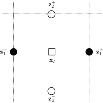
Fig. 1: The virtual collocation points $\mathbf{z}_{J,i}^{\pm}$ and the virtual node point $\mathbf{x}_{I}$.

For the stability and convergence of virtual interpolation scheme, we assume that dilation parameter $\rho$ of window function of Theorem 2.1 is comparable to the node interval $h$, namely, there is $C$ satisfying

$$0<\rho<Ch.$$

If we let $(\mathbf{v},q)$ the true solution in $H^{1}_{per}(\Omega)\times L^{2}_{per}(\Omega)$, then

$$\|\mathbf{v}\|_{H^{1}(\Omega)}+\|q\|_{L^{2}(\Omega)}\leq C\|\mathbf{f}\|_{H^{-1}(\Omega)}.$$

In case of periodic domain with regular node set, the continuous projection operator $K$ is a convolution of the kernel $k_{\rho}$ (see equation (3)) and thus we have

$$-\Delta K\mathbf{v}+\nabla Kq=K\mathbf{f}\quad\mbox{and}\quad\mbox{div}K\mathbf{v}=0,$$

and the stability of continuous projection follows from the energy estimate:

Theorem 3.3.

Let $(\mathbf{u},q)\in H_{per}^{1}(\Omega)\times L^{2}_{per}(\Omega)$, $(\mathbf{v},q)$ are a solution of (1) and $K$ is the continuous projection operator in ((3)) then we have an inequality:

$$\|K\mathbf{v}-\mathbf{v}\|_{H^{1}}+\|Kq-q\|_{L^{2}}\leq C\|K\mathbf{f}-\mathbf{f}\|_{H^{-1}}.$$

The analysis of discrete projection $\Gamma$ for $\mathbf{v}$ and $p$ is more complicated. Let us assume that the reproducing degree $m$ in (2) is greater than or equal to 2 and polynomials of degree two can be reproduced.

We suppose $\mathbf{v}\in C^{2,\alpha}$ for a $\alpha>0$. For fixed $\mathbf{x}_{I}$, we have Taylor expansion if $|\mathbf{x}-\mathbf{x}_{I}|\leq\rho\leq Ch$:

$$\mathbf{v}(\mathbf{x})=\mathbf{v}(\mathbf{x}_{I})+\nabla\mathbf{v}(\mathbf{x}_{I})(\mathbf{x}-\mathbf{x}_{I})+\frac{1}{2}\nabla^{2}\mathbf{v}(\mathbf{x}_{I})(\mathbf{x}-\mathbf{x}_{I})^{2}+C\|\nabla^{2}\mathbf{v}\|_{C^{\alpha}}O(h^{2+\alpha}),$$

and from the reproducing property

$$\Gamma\mathbf{v}(\mathbf{x})=\mathbf{v}(\mathbf{x}_{I})+\nabla\mathbf{v}(\mathbf{x}_{I})(\mathbf{x}-\mathbf{x}_{I})+\frac{1}{2}\nabla^{2}\mathbf{v}(\mathbf{x}_{I})(\mathbf{x}-\mathbf{x}_{I})^{2}+C\|\nabla^{2}\mathbf{v}\|_{C^{\alpha}}O(h^{2+\alpha}),$$

and

$$(A\Gamma\mathbf{v})_{I}=(D^{*}D(\Gamma\mathbf{v}))_{I}=\Delta\mathbf{v}(\mathbf{x}_{I})+O(h^{\alpha}).$$

We have that

$$\Gamma v_{1,x_{1}}(\mathbf{x}) =v_{1,x_{1}}(\mathbf{x}_{I})+v_{1,x_{1}x_{1}}(\mathbf{x}_{I})(x_{1}-x_{I,1})+v_{1,x_{1}x_{2}}(\mathbf{x}_{I})(x_{2}-x_{I,2})+C\|\nabla^{2}\mathbf{v}\|_{C^{\alpha}}O(h^{1+\alpha})$$

$$\Gamma v_{2,x_{2}}(\mathbf{x}) =v_{2,x_{2}}(\mathbf{x}_{I})+v_{2,x_{2}x_{2}}(\mathbf{x}_{I})(x_{2}-x_{I,2})+v_{2,x_{1}x_{2}}(\mathbf{x}_{I})(x_{1}-x_{I,1})+C\|\nabla^{2}\mathbf{v}\|_{C^{\alpha}}O(h^{1+\alpha}),$$

and we also have that, from divergence free condition,

$$v_{1,x_{1}x_{2}}(\mathbf{x}_{I})(x_{2}-x_{I,2}) +v_{2,x_{2}x_{2}}(\mathbf{x}_{I})(x_{2}-x_{I,2})=0$$

$$v_{2,x_{1}x_{2}}(\mathbf{x}_{I})(x_{1}-x_{I,1}) +v_{1,x_{1}x_{1}}(\mathbf{x}_{I})(x_{1}-x_{I,1})=0.$$

Taking divergence of $\Gamma\mathbf{v}$ and noting that $\nabla(\mbox{div}\mathbf{v})(\mathbf{x}_{I})=0$, we also have

$$\mbox{div}\Gamma\mathbf{v}(\mathbf{x}_{I})=\|\nabla^{2}\mathbf{v}\|_{C^{\alpha}}O(h^{1+\alpha}),$$

and similarly from mean value theorem

$$(D^{*}\Gamma\mathbf{v})_{I}=\|\nabla^{2}\mathbf{v}\|_{C^{\alpha}}O(h^{1+\alpha}).$$

Similarly, we suppose $q\in C^{1,\alpha}$ and we have

$$(\nabla\Gamma q)(\mathbf{x}_{I})=\nabla q(\mathbf{x}_{I})+\|\nabla q\|_{C^{\alpha}}O(h^{\alpha}),$$

and from mean value theorem

$$\|(D\Gamma q)_{I}-\nabla\Gamma q(\mathbf{x}_{I})\|\leq C\|\nabla q\|_{C^{\alpha}}h^{\alpha}.$$

Since $-\Delta\mathbf{v}(\mathbf{x}_{I})+\nabla q(\mathbf{x}_{I})=\mathbf{f}(\mathbf{x}_{I})$ and $\mathbf{f}\in C^{\alpha}$ we have the error equation for virtual interpolation method,

(6) $$-A(U-\Gamma\mathbf{v})+D(P-\Gamma q) =(F-\Gamma\mathbf{f})+(\|\nabla^{2}\mathbf{v}\|_{C^{\alpha}}+\|\nabla q\|_{C^{\alpha}})O(h^{\alpha}),$$

$$D^{*}(U-\Gamma\mathbf{v}) =\|\nabla^{2}\mathbf{v}\|_{C^{\alpha}}O(h^{1+\alpha})=\|\mathbf{f}\|_{C^{\alpha}}O(h^{1+\alpha}).$$

where $(U,P)$ are solution of the discrete Stokes equations (4).

Theorem 3.4.

We suppose that all the node sets satisfy the conditions in Theorem 3.1, and the reproducing degree $m\geq 2$. We also assume that $\mathbf{f}\in C^{\alpha}$. We let $(\mathbf{v},q)$ the true solution in $C^{2,\alpha}_{per}(\Omega)\times C^{1,\alpha}_{per}(\Omega)$ and $(U,P)$ discrete solution. Then, there is an absolute constant $C$ such that

$$\|D(U-\Gamma\mathbf{v})\|_{l^{2}}+\|P-\Gamma q\|_{l^{2}}\leq Ch^{\alpha-1}\|\mathbf{f}\|_{C^{\alpha}(\Omega)}.$$

Proof.

If we have $\mathbf{f}\in C^{\alpha}$, from Calderon-Zygmund theory of Stokes equations we have $\mathbf{v}\in C^{2,\alpha}$ and $q\in C^{1,\alpha}$. From Sobolev embedding we have

$$\|\nabla^{2}\mathbf{v}\|_{C^{\alpha}}+\|\nabla q\|_{C^{\alpha}}\leq C\|\mathbf{f}\|_{C^{\alpha}},$$

and in case $\mathbf{f}\in C^{\alpha}$, we have

$$\|F-\Gamma\mathbf{f}\|_{l^{\infty}}\leq Ch^{\alpha}\|\mathbf{f}\|_{C^{1,\alpha}}.$$

The $(U,P)$ satisfies the discrete Stokes equations (4) and therefore we have error equation (6) for $(E,R)=(U-\Gamma\mathbf{v},P-\Gamma q)$ such that at each $\mathbf{x}_{I}$

$$(-AE+DR)_{I}=O(h^{\alpha})\|\mathbf{f}\|_{C^{\alpha}}\quad\mbox{and}\quad D^{*}E_{I}=O(h^{1+\alpha})\|\mathbf{f}\|_{C^{\alpha}}.$$

By the discrete Poincaré inequality (see [11]), with the condition $\sum_{I}E_{I}=0$, we have

$$\|E\|_{l^{2}}\leq C\|DE\|_{l^{2}}.$$

Then simply applying $E$ to error equation and considering ellipticity of discrete operator $A$, we prove that

(7) $$\|DE\|_{l^{2}}^{2}\leq Ch^{\alpha-1}\|\mathbf{f}\|_{C^{\alpha}}\|R\|_{l^{2}}+Ch^{2\alpha-2}\|\mathbf{f}\|^{2}_{C^{\alpha}}.$$

From inf-sup condition (see 3.1), we find $W\in\mathbb{R}^{2M}$ such that

$$\|R\|_{l^{2}}\leq C\frac{\langle D^{*}W,R\rangle}{\|DW\|_{l^{2}}}.$$

Applying $W$ to error equation and we obtain from inf-sup condition

$$C\|R\|_{l^{2}}\|DW\|_{l^{2}}\leq\langle D^{*}W,R\rangle=\langle DW,DE\rangle+O(h^{\alpha-1})\|\mathbf{f}\|_{C^{\alpha}}\|DW\|_{l^{2}}.$$

Therefore we conclude

$$\|R\|_{l^{2}} =\frac{1}{\|DW\|_{l^{2}}}\left(\langle DW,DE\rangle+O(h^{\alpha-1})\|\mathbf{f}\|_{C^{\alpha}}\|DW\|_{l^{2}}\right)$$

$$\leq C\|DE\|_{l^{2}}+Ch^{\alpha-1}\|\mathbf{f}\|_{C^{\alpha}.}$$

and from Cauchy-Schwarz inequality on the error of pressure $R$ term of (7) we prove the theorem. ∎

Remark 3.5.

Our theorem, 3.4 implies that

$$h^{2}\|D(U-\Gamma\mathbf{v})\|^{2}_{l^{2}} +h^{2}\|P-\Gamma q\|^{2}_{l^{2}}$$

$$=\int_{\Omega}\left|\overline{D(U-\Gamma\mathbf{v})}\right|^{2}+\left|\overline{P-\Gamma\mathbf{q}}\right|^{2}d\mathbf{x}$$

$$\leq Ch^{2\alpha}\|\mathbf{f}\|_{C^{\alpha}}^{2}.$$

4 Numerical examples

In this section we present a series of test problems of increasing complexity to demonstrate the accuracy and robustness of the VIP method.

4.1 Spatial convergence test

We consider the Kovasznay flow, which is steady problem with analytic expression. The velocity and pressure fields are given by the following equations,

$$u(x,y) =1-e^{\lambda x}\cos(2\pi y),$$

$$v(x,y) =\frac{\lambda}{2\pi}e^{\lambda x}\sin(2\pi y),$$

$$p(x,y) =\frac{1}{2}\left(1-e^{2\lambda x}\right),$$

where $\lambda=\frac{Re}{2}-\left(\frac{Re^{2}}{4}+4\pi^{2}\right)^{1/2}$ with $Re=40$. We consider the Kovasznay flow on the domain $\Omega=[-0.5,1.5]\times[0,2]$, which is discretized with regular nodes. Fig. 2(d) shows the discrete norms of the errors in the velocity and pressure with the analytical solutions. The contour lines for $u$-velocity, $v$-velocity, and pressure are shown in Fig. 2(a)-(c).

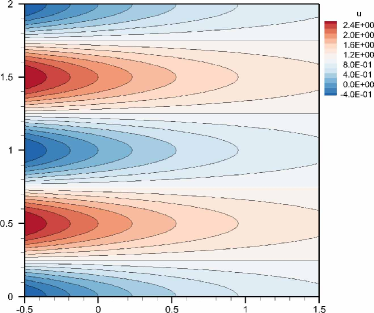
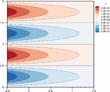
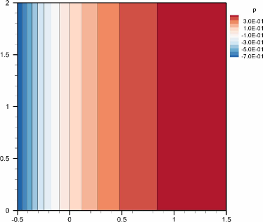
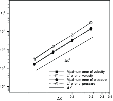
Fig. 2: Kovasznay flow : (a) $u$-velocity; (b) $v$-velocity; (c) pressure; (d) the convergence of the numerical solutions from the uniform nodes.

4.2 Lid-driven cavity flow

The next test is a two-dimensional lid-driven cavity problem on the domain $\Omega=[0,1]\times[0,1]$ with $(u,v)=(1,0)$ on the top and no-slip boundary conditions on the rest part of the boundary. Figure 3(d) and Figure 4(d) show the centerline velocities $u(y)\mbox{ and }v(x)$ along the vertical and horizontal centerlines, respectively. Reynolds numbers of $Re=100\mbox{ and }400$ are chosen for validating the current method. The present result is in good agreement with that of Ghia et al. [8] who used 128$\times$128 uniformly distributed rectangular cells. The contour lines for stream function, pressure, and vorticity are shown in Fig 3(a)-(c) and Fig 4(a)-(c).

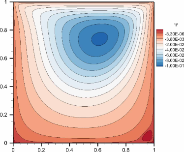
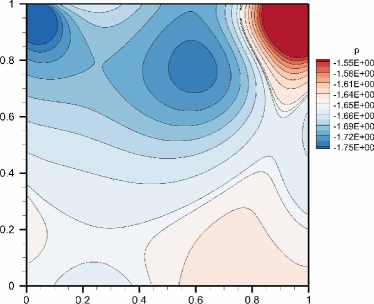
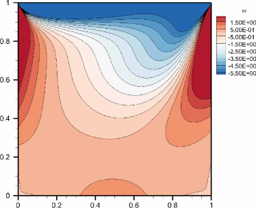
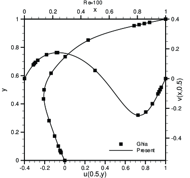
Fig. 3: Lid-driven cavity flow with $Re=100$ : (a) stream function; (b) pressure; (c) vorticity; (d) centerline velocities $u$ and $v$. Results from Ghia et al. [8] are compared with current numerical solutions.

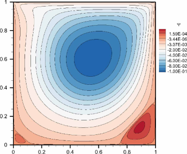
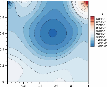
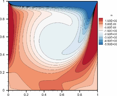
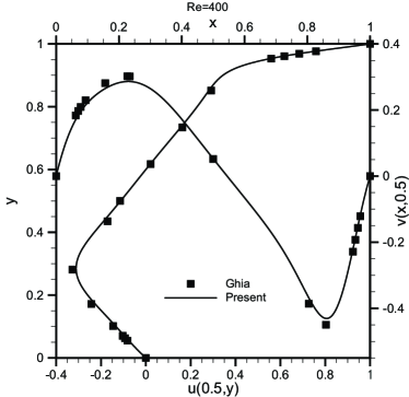
Fig. 4: Lid-driven cavity flow with $Re=400$ : (a) stream function; (b) pressure; (c) vorticity; (d) centerline velocities $u$ and $v$. Results from Ghia et al. [8] are compared with current numerical solutions.

4.3 Flow over a circular cylinder

We consider flow over a circular cylinder as another test problem because the dimensions of the recirculation zone and the force on the cylinder at various Reynolds numbers are readily available from previous experimental and numerical studies. Our two-dimensional simulations are performed by introducing a cylinder of diameter d = 1 in a large computational domain D with initially uniform flow, $u=u_{\infty}=1$. Reynolds numbers of $Re=10,\,20,\mbox{ and }40$ are chosen for validating the current method at steady-state. The resulting wake dimensions and drag coefficients are compared to values reported in the literatures [5, 17, 7, 6, 10]. In Fig. 5, the vorticity and the pressure coefficient $C_{p}$ on the body surface are plotted, while Table 1 shows the drag coefficient($C_{D}$) for each Reynolds number of 10, 20, and 40. The stream function and vorticity contours around the body are also illustrated in Fig. 6.

$C_{D}$	$Re=10$	$Re=20$	$Re=40$
Dennis et al.[5]	2.85	2.05	1.522
Takami et al.[17]	2.80	2.01	1.536
Tuann et al.[18]	3.18	2.25	1.675
Fornberg[7]		2.00	1.498
H. Ding[6]	3.07	2.18	1.713
Kim et al.[10]			1.51
Present	3.03	2.17	1.536

Table 1: Comparison of drag coefficient for steady flow.

(a) Wall pressure coefficient ($C_{p}$).

(b) Wall vorticity ($\omega$) for

Fig. 5: Comparison of the vorticity and the pressure coefficients on the circular cylinder with $Re=10,20$ and $40$.

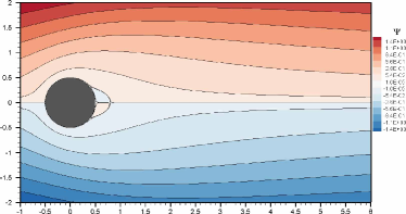
(a) Stream functions for $Re=10$

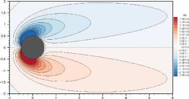
(b) Vorticity for $Re=10$

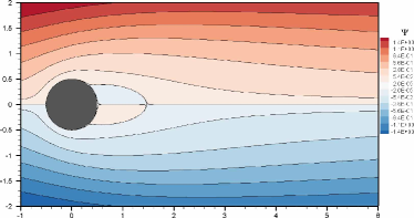
(c) Stream function for $Re=20$

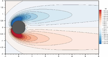
(d) Vorticity for $Re=20$

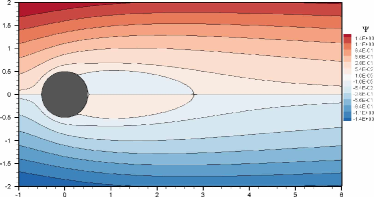
(e) Stream functions for $Re=40$

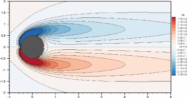
(f) Vorticity for $Re=40$

Fig. 6: Stream function and vorticity of flow over a circular cylinder with $Re=10,20$, and $40$.

References

• [1] Ivo Babuška, The finite element method with Lagrangian multipliers, Numerische Mathematik, 20 (1973), pp. 179–192.
• [2] F Brezzi, On the existence, uniqueness and approximation of saddle-point problems arising from lagrangian multipliers, ESAIM: Mathematical Modelling and Numerical Analysis - Modélisation Mathématique et Analyse Numérique, 8 (1974), pp. 129–151.
• [3] Hi Jun Choe, Mu-Young Ahn, Ki Dong Song, Kyong-Yop Park, and Seong-Kwan Park, Flow Field Computation for Simplified High Voltage Gas Circuit Breaker Model by Upwind Meshfree Method, Japanese Journal of Applied Physics, 45 (2006), pp. 9247–9253.
• [4] Hi Jun Choe, Yongsik Kim, and Do Wan Kim, Meshfree method for the non-stationary incompressible Navier-Stokes equations, Discrete and Continuous Dynamical Systems - Series B, 6 (2006), pp. 17–39.
• [5] S. C. R. Dennis and Gau-Zu Chang, Numerical solutions for steady flow past a circular cylinder at Reynolds numbers up to 100, J. Fluid Mech., 42 (2006), p. 471.
• [6] H. Ding, C. Shu, K.S. Yeo, and D. Xu, Simulation of incompressible viscous flows past a circular cylinder by hybrid FD scheme and meshless least square-based finite difference method, Comput. Methods Appl. Mech. Eng., 193 (2004), pp. 727–744.
• [7] Bengt Fornberg, A numerical study of steady viscous flow past a circular cylinder, Journal of Fluid Mechanics, 98 (2006), p. 819.
• [8] U Ghia, K.N Ghia, and C.T Shin, High-Re solutions for incompressible flow using the Navier-Stokes equations and a multigrid method, J. Comput. Phys., 48 (1982), pp. 387–411.
• [9] Vivette Girault and Pierre-Arnaud Raviart, Finite Element Methods for Navier-Stokes Equations: Theory and Algorithms. Springer Series in Computational Mathematics (Book 5), Springer-Verlag, Berlin, 1986.
• [10] Jungwoo Kim, Dongjoo Kim, and Haecheon Choi, An Immersed-Boundary Finite-Volume Method for Simulations of Flow in Complex Geometries, J. Comput. Phys., 171 (2001), pp. 132–150.
• [11] Anh Ha Le and Pascal Omnes, Discrete Poincaré inequalities for arbitrary meshes in the discrete duality finite volume context, Electron. Trans. Numer. Anal., 40 (2013), pp. 94–119.
• [12] Wing Kam Liu, Yijung Chen, R.Aziz Uras, and Chin Tang Chang, Generalized multiple scale reproducing kernel particle methods, Comput. Methods Appl. Mech. Eng., 139 (1996), pp. 91–157.
• [13] Wing-Kam Liu, Shaofan Li, and Ted Belytschko, Moving least-square reproducing kernel methods (I) Methodology and convergence, Comput. Methods Appl. Mech. Eng., 143 (1997), pp. 113–154.
• [14] Seong-Kwan Park, Flow field computation of compressible Euler equations in time varying domain, ph.d thesis, Yonsei University, Seoul, Korea, 2010.
• [15] Seong-Kwan Park, Kyong-Yop Park, and Hi Jun Choe, Flow field computation for the high voltage gas blast circuit breaker with the moving boundary, Computer Physics Communications, 177 (2007), pp. 729–737.
• [16] Dongho Shin and John C Strikwerda, Inf-sup conditions for finite-difference approximations of the stokes equations, J. Aust. Math. Soc. Ser. B. Appl. Math., 39 (2009), p. 121.
• [17] Hideo Takami, Steady Two-Dimensional Viscous Flow of an Incompressible Fluid past a Circular Cylinder, Phys. Fluids, 12 (1969), pp. II–51.
• [18] Shih-yu Tuann and Mervyn D. Olson, Numerical studies of the flow around a circular cylinder by a finite element method, Comput. Fluids, 6 (1978), pp. 219–240.