Temporal and spatial heterogeneity in aging colloids: a mesoscopic model

Abstract

A model of dense hard sphere colloids building on simple notions of particle mobility and spatial coherence is presented and shown to reproduce results of experiments and simulations for key quantities such as the intermediate scattering function, the particle mean-square displacement and the $\chi_{4}$ mobility correlation function. All results are explained by two emerging and interrelated dynamical properties: i) a rate of intermittent events, quakes, which decreases as the inverse of the system age $t$, leading to $\mu_{{\rm q}}(t_{{\rm w}},t)\propto\log(t/t_{{\rm w}})$ as the average number of quakes occurring between the ‘waiting time’ $t_{{\rm w}}$ and the current time $t$; ii) a length scale characterizing correlated domains, which increases linearly in $\log t$. This leads to simple and accurate scaling forms expressed in terms of the single variable, $t/t_{{\rm w}}$, preferable to the established use of $t_{{\rm w}}$ and of the lag time $\tau=t-t_{{\rm w}}$ as variables in two-point correlation functions. Finally, we propose to use $\chi_{4}\left(t_{{\rm w}},t\right)$ experimentally to extract the growing length scale of an aging colloid and suggest that a suitable scaling of the probability density function of particle displacement can experimentally reveal the rate of quakes.

Aging is a spontaneous off-equilibrium relaxation process, which entails a slow change of thermodynamic averages. In amorphous materials with quenched disorder Struik (1978); Nordblad et al. (1986); Rieger (1993); Kob et al. (2000); Crisanti and Ritort (2004); Sibani and Jensen (2005), measurable quantities such as the thermo-remanent magnetization G.G. Kenning, G.F. Rodriguez and R. Orbach (2006) and the thermal energy Crisanti and Ritort (2004); P. Sibani (2007); Sibani and Christiansen (2008); Christiansen and Sibani (2008) decrease, on average, at a decelerating rate during the aging process. In dense colloidal suspensions, light scattering Cipelletti et al. (2000); Masri et al. (2005) and particle tracking techniques Weeks et al. (2000); Courtland and Weeks (2003); Lynch et al. (2008); Candelier et al. (2009) have uncovered intermittent dynamics and a gradual slowing down of the rate at which particles move. Intermittency suggest a hierarchical dynamics, instead of coarsening, as the origin of this process. However, changes in spatially averaged quantities such as energy and particle density are difficult to measure and the question of which physical properties are actually evolving in an aging colloid Hentschel et al. (2007); Cianci et al. (2006) lacks a definite answer.

In a recent paper Boettcher and Sibani (2011), two of the authors proposed that kinetic constraints bind colloidal particles together in ‘clusters’. As long as a cluster persists, its center of mass position remains fixed, on average, but once it breaks down the particles which belong to it can move independently in space, and are able to join other clusters. The dynamics is controlled by the probability per unit of time, $P(h)$, that a cluster of size $h$ collapses through a quake. Specifically, if the cluster-collapse probability is exponential, as in Eq. (1) below, quakes follow a Poisson process whose average is proportional to the logarithm of time. Log-Poisson processes describe the aging phenomenology of a wide class of glassy systems Crisanti and Ritort (2004); P. Sibani (2007); Sibani and Christiansen (2008); Christiansen and Sibani (2008); G.G. Kenning, G.F. Rodriguez and R. Orbach (2006) and, specifically in our case, imply that particle motion is (nearly) diffusive on a logarithmic time scale, as found in our analysis Boettcher and Sibani (2011) of tracking experiments Courtland and Weeks (2003).

In this Letter, we introduce a model of cluster dynamics based on these principles that explicitly accounts for the spatial form of the clusters on a lattice in any dimension. This enables us to calculate the internal energy, the intermediate scattering function, the mean square displacement, the mobility correlation function $\chi_{4}$ and other measures of spatial complexity. We can hence compare with simulational Masri et al. (2010) and experimental Berthier et al. (2005); Berthier (2011) data, and suggest a number of experiments to probe colloidal dynamics.

Our particles reside on a lattice with periodic boundary conditions, each lattice site occupied by exactly one particle. Particles are either mobile singletons (cluster-size $h=1$) or form immobile contiguous clusters of size $h>1$. When picked for an update, mobile particles exchange position with a randomly selected neighbor and join that neighbor’s cluster. If the particle is not mobile, either its entire cluster “shatters” into $h$ newly mobile particles with probability

$$P\left(h\right)=e^{-h},$$ (1)

or no action is taken. When starting with an initial state consisting of singletons, i.e., without any structure, the model develops spatially heterogeneous clusters with a length scale growing logarithmically in time. The state of the system on a square lattice with $L=256$ after $10^{15}$ sweeps is depicted in Fig. 1(a) while Fig. 1(b) shows the logarithmic growth of the average cluster size.

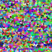
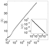
Figure 1: (a) Snapshot of a $256\times 256$ system after $t=10^{15}$ sweeps. Random colors are assigned to different clusters for visibility. Cluster sizes apparently are peaked around some average value $\langle h\rangle\sim\log t$, as shown in (b). The decelerating rate $\lambda(t)\sim 1/t$ of cluster break-up events that emerges from the probability in Eq. (1) is shown in the inset.

As previously shown Boettcher and Sibani (2011), the rate of events decelerates as $1/t$, see inset of Fig. 1(b), which makes random-sequential updates inefficient. In our simulations, we therefore use the Waiting Time Method Bortz et al. (1975); Dall and Sibani (2001), where a random “lifetime” is assigned to each cluster based on the geometric distribution associated with $P(h)$; the cluster with the shortest remaining lifetime is shattered and lifetimes for other pre-existing or newly formed clusters are adjusted or newly assigned, following the Poisson statistics. With this event-driven algorithm, we have been able to follow our model evolution over 15 decades in time, far exceeding current experimental time windows.

Important aspects of aging dynamics are described by observable quantities with two time arguments. Here, we denote by $t$ the current time and by $t_{{\rm w}}$ the waiting time before measurements are taken for a system initialized at $t=0$. To conform to common usage, the lag time $\tau\equiv t-t_{{\rm w}}$ is used as abscissa in the main plot of relevant figures. However, we also provide a collapse of the data, which is best accomplished when global time $t$ is scaled by $t_{{\rm w}}$ as independent time variable.

Using the details of the Lennard-Jones potential in their molecular dynamics simulation, El-Masri et al. Masri et al. (2010) were able to determine the evolution of the internal energy of a colloidal system in terms of its pressure. We simply monitor the interface between clusters as a proxy of the internal energy, assuming that a shrinking interface indicates a decline in free volume which allows particles within clusters to relieve their mutual repulsion. The average number of clusters $\langle n\rangle$ can be written in terms of average cluster size $\langle h\rangle$ as $\langle n\rangle=L^{2}/\langle h\rangle$. Since the average cluster size increases with $\langle h\rangle\sim\log(t)$, see Fig. 1(b), and since for compact clusters in two dimensions the interface-length scales as $S(h)\propto\sqrt{\langle h\rangle}$, the average energy per particle $\left\langle e_{{\rm Int}}\right\rangle$ is estimated as

$$\left\langle e_{{\rm Int}}\right\rangle=S(h)\frac{\langle n\rangle}{L^{2}}\sim\frac{1}{\sqrt{\langle h\rangle}}\sim\frac{1}{\sqrt{\log t}}.$$ (2)

Fig. 2 shows that the approximation holds after a more rapid initial decay. The slow decay matches that of the Lennard-Jones simulations in Fig. 1 of Ref. Masri et al. (2010), and it is reminiscent of granular compactification Ben-Naim et al. (1998), where noisy tapping slowly anneals away excess free volume. The same process drives our cluster growth, although density changes are not explicitly expressed in the model.

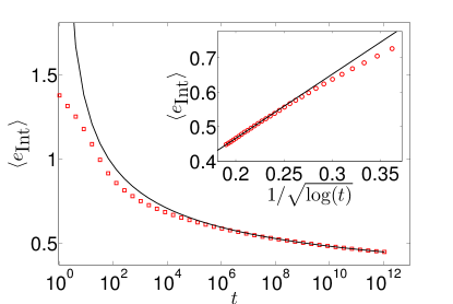
Figure 2: Average interface energy per particle, $\left\langle e_{{\rm Int}}\right\rangle$, for $L=64$. For large $t$, the interface energy follows the form $\left\langle e_{{\rm Int}}\right\rangle\sim 1/\sqrt{\log(t)}$ derived in Eq. (2), as confirmed by the inset.

Readily available through light scattering experiments, the self-intermediate scattering function (SISF) $f_{s}$ assesses two-time correlations used to resolve dynamical characteristics of non-equilibrium systems. Formally, it is defined as the spatial Fourier transform,

$$f_{s}\left(\vec{\textbf{q}},t_{{\rm w}},t\right)=\int d\vec{\textbf{r}}\,\mathcal{G}_{s}\left(\vec{\textbf{r}},t_{{\rm w}},t\right)\exp\left[-i\vec{\textbf{q}}\cdot\vec{\textbf{r}}\right],$$ (3)

of the self-part of the van Hove distribution function,

$$\mathcal{G}_{s}\left(\vec{\textbf{r}},t_{{\rm w}},t\right)=\frac{1}{N}\sum_{j}\delta\left[\vec{\textbf{r}}-\Delta\vec{\textbf{r}}_{j}\right],$$ (4)

with $\Delta\vec{\textbf{r}}_{j}\left(t_{{\rm w}},t\right)=\vec{\textbf{r}}_{j}\left(t\right)-\vec{\textbf{r}}_{j}\left(t_{{\rm w}}\right)$ as displacement of particles $j$ in the time interval between $t_{{\rm w}}$ and $t$. In general, SISF can be interpreted as a measure of the “reciprocal of movement”, meaning the average tendency of particles to stay confined in cages whose size scales with inverse magnitude of the wave vector $\vec{\textbf{q}}$. Using symmetry and the integer values of the positions, the discrete version of SISF reduces to

$$f_{s}(q,t_{{\rm w}},t)=\left\langle\frac{1}{N}\sum_{j=1}^{N}\cos\left(\vec{\textbf{q}}\cdot\Delta\vec{\textbf{r}}_{j}\right)\right\rangle.$$ (5)

Due to spatial isotropy, the SISF is only a function of the magnitude $q$, with $q_{{\rm min}}=2\pi/L\leq q\leq\pi\sqrt{2}=q_{{\rm max}}$.

Figure 3 shows the results of simulating an $L=64$ system using $2000$ instances and waiting times varying from $2^{10}$ to $2^{18}$ in powers of two. Panel $(a)$ depicts the behavior of SISF as a function of lag time. For large $t_{{\rm w}}$, to a good approximation the data can be represented by a power law of the scaling variable $\hat{t}=\log\left(t/t_{{\rm w}}\right)$, $f_{s}\sim C\hat{t}^{-A}$, where $C$ is a constant and $A$ a positive, non-universal exponent, see panel $(b)$ of Fig. 3. Some curvature remains, nevertheless, and data do not completely collapse. In contrast, panel $(c)$ achieves excellent scaling and collapse using the form (discussed later)

$$f_{s}\propto\exp\big{\{}-A\hat{t}\left(1-\epsilon\hat{t}\right)\big{\}},$$ (6)

with $\epsilon\approx 0.012$. The power-law exponent $A\approx 0.1$ weakly depends on $t_{{\rm w}}$ and changes systematically by about $40\%$ over two decades of $t_{{\rm w}}$, likely reflecting the effect of higher order corrections in Eq. (6). Note that $A$ is comparable to the same exponent found in expensive Lennard-Jones simulations, see Fig. 2 of Ref. Masri et al. (2010).

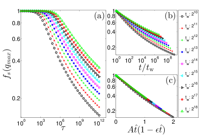
Figure 3: Decay of SISF at $q_{{\rm max}}=\sqrt{2}\pi$ and system size $L=64$ for $t_{{\rm w}}=2^{k}$, $k=10,11,\ldots,18$, using three different forms of independent variable: $(a)$ the lag time $\tau$, $(b)$ the total run time $t$ scaled by waiting time $t_{{\rm w}}$, and $(c)$ the correction to $\hat{t}=\log(t/t_{{\rm w}})$ in Eq. (6) (see text for details). The fitted values $A$ and $\epsilon$ remain approximately constant across the range of different $t_{{\rm w}}$; with $A\approx 0.1$ and a correction of merely $\epsilon\approx 1$%.

An alternative characterization of immobility, persistence, measures the average fraction of particles that never move Boettcher and Sibani (2011); Pastore et al. (2011). Conceptually simple and easily accessible in simulations, persistence must be deduced indirectly in experiments from the SISF at its peak wave-vector. In terms of Eq. (4), persistence is defined as

$$\mathcal{P}\left(t_{{\rm w}},t\right)=\mathcal{G}_{s}\left(\left|\vec{\textbf{r}}\right|\leq d,t_{{\rm w}},t\right),$$ (7)

i.e., the fraction of particles that have coordinates at times $t_{{\rm w}}$ and $t$ with $\lvert\vec{\textbf{r}}(t)-\vec{\textbf{r}}(t_{{\rm w}})\rvert\leq d$, where $d$ is a threshold representing the largest distance a particle can move without detection. For small $d$, the SISF in Eq. (5) reduces to persistence for $\lvert\vec{\textbf{q}}\rvert\rightarrow\infty$. To avoid over-counting particles that return to their original position, in simulations we only count particles that have been activated since $t_{{\rm w}}$. Our results for persistence with $d=1$ are virtually indistinguishable from those for SISF at $q_{{\rm max}}$ in Fig. 3. Figure 4 illustrates the recurrance of quake activity to sites on a $L=64$ lattice for a time interval $[t_{{\rm w}},4t_{{\rm w}}]$ with $t_{{\rm w}}=2^{12}$. While most particles persist in their position, mobility concentrates in areas scattered about the system (“dynamic heterogeneities”Weeks et al. (2000)) with future activity favoring previously mobile sites.

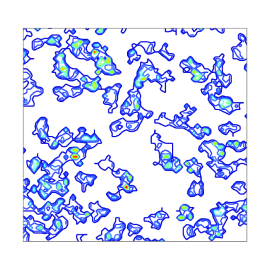
Figure 4: Persistence on a $64\times 64$ lattice. For times $t$ from $t_{{\rm w}}=2^{12}$ to $4t_{{\rm w}}$ activations are recorded. Within a dominant inert background (white), domains are encircled with darker to lighter contours to mark one to ten activations. This mobility pattern demonstrates dynamic heterogeneity and the associated the preferential return of activity to the same sites.

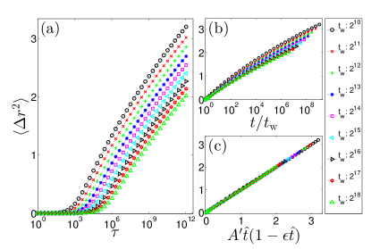
Figure 5: MSD for a range of different waiting times and different choices of independent variable. The system parameters are the same as in Fig. 3.

The positional variance or mean square displacement (MSD) between times $t_{{\rm w}}$ and $t$ is computed by averaging the square displacement, first over of all particles and then over the ensemble. Using $\left\langle\cdot\right\rangle$ for the ensemble average and $\lvert\cdot\rvert$ for the Euclidean norm, the MSD is written as

$$\Delta r^{2}(t_{{\rm w}},t)=\left\langle\frac{1}{N}\sum_{j=1}^{N}\lvert\vec{\textbf{r}}_{j}(t)-\vec{\textbf{r}}_{j}(t_{{\rm w}})\rvert^{2}\right\rangle.\$$ (8)

Figure 5 shows the MSD for a system of size $L=64$ with waiting times $t_{{\rm w}}=2^{k}$ for $k=10,11\ldots 18$. In analogy with Fig. 3, the MSD is plotted vs. three different variables: Panel $(a)$ uses the lag time, panel $(b)$ the scaling variable $t/t_{{\rm w}}$, and panel $(c)$ uses the same type of correction as in Eq. (6), that is, $\Delta r^{2}\propto A^{\prime}\hat{t}\left(1-\epsilon\hat{t}\right)$ with the same $\epsilon=0.012$ and the “log-diffusion” constant $A^{\prime}\approx 0.2$. Note that a system aged up to time $t_{{\rm w}}$ has a “plateau” of inactivity for lag times up to $\tau\sim t_{{\rm w}}$. These plateaus, often associated with the “caging” of particles Weeks et al. (2000), are easily removed with $t/t_{{\rm w}}$ as independent variable, see Fig. 5(b), leading to the approximate scaling behavior $\Delta r^{2}\sim\log(t/t_{{\rm w}})$ and a reasonable data collapse. The residual curvature is removed altogether in panel $(c)$ using the same correction as in Fig. (3), $\epsilon=0.012$, but a constant $A^{\prime}\approx 0.2$ that is unrelated to $A$.

To gauge correlated spatial fluctuation and dynamical heterogeneity, we consider the 4-point susceptibility Berthier (2011)

$$\chi_{4}(t_{{\rm w}},t)=\langle M(t_{{\rm w}},t)^{2}\rangle-\langle M(t_{{\rm w}},t)\rangle^{2},$$ (9)

with mobility measure $M(t_{{\rm w}},t)=\sum_{j}c_{j}(t_{{\rm w}},t)$, $c_{j}(t_{{\rm w}},t)=\exp\left\{-\lvert\lvert\vec{\textbf{r}}_{j}(t)-\vec{\textbf{r}}_{j}(t_{{\rm w}})\rvert\rvert_{1}\right\}$, where $\lvert\lvert\cdot\rvert\rvert_{1}$ denotes the Manhattan norm. Figure 6 shows $\chi_{4}$ vs. $t$ for a range of waiting times $t_{{\rm w}}$. While the data does not allow a global collapse, the logarithmic increase in peak-height vs. $t_{{\rm w}}$ is clearly visible. This is expected since, by model construction, heterogeneous dynamics is mainly due to the collapse of clusters, locked in at a typical size $h\sim\log t_{{\rm w}}$, that re-mobilizes a corresponding number of particles at a time $t_{{\rm peak}}>t_{{\rm w}}$, which is reflected in the height of the peak. Fig. 6 is reminiscent of results in Ref. Berthier et al. (2005) for experiments and simulations, where $\chi_{4}$ is measured for a sequence of equilibrium states prepared ever closer to jamming, either by increasing density or decreasing temperature.

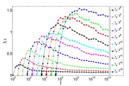
Figure 6: Plot of $\chi_{4}$ as a function of time $t$ for various $t_{{\rm w}}$ at $L=64$. Note that the peak-height increases with $\log t_{{\rm w}}$.

In summary, our model coarse-grains away the “in-cage rattling” of particles while incorporating time intermittency and spatial heterogeneity. Its behavior, which qualitatively accounts for relevant experimental findings, can be described analytically using the log-Poisson statistics of cluster collapses Boettcher and Sibani (2011).

Two-point averages have been plotted versus the lag time, $\tau=t-t_{{\rm w}}$, to adhere to the established usage and, in insets, versus the scaled variable $t/t_{{\rm w}}$. The first choice lacks a theoretical basis in the absence of time translational invariance. The second indicates that the distinction between an early dynamical regime $\tau<t_{{\rm w}}$ and an asymptotic aging regime $\tau>t_{{\rm w}}$ is moot.

Deviations from $\log(t/t_{{\rm w}})$-scaling are visible at long times in both the MSD and the SISF (or, equivalently, the persistence). Interestingly, experimental data show a similar behavior, see Fig. 1 in Ref. Boettcher and Sibani (2011) and Fig. 4 in Ref. Masri et al. (2010). As shown in the insets, these deviations can be eliminated by a new scaling variable with a small ($\epsilon\approx 1$%) correction in $\log(t/t_{{\rm w}})$, whose origin is as follows: Consider first the fraction of persistent particles $p_{n}$ after $n$ quakes (marked white in Fig. 4), and neglect that the size of a quake slowly increases with cluster size and that particle hits are not uniformly spread throughout the system. That persistence curve $p_{n}$ then decays exponentially with $n$. Averaging $p_{n}$ over the Poisson distribution of $n$ gets

$${\cal P}(t_{{\rm w}},t)=\exp(-A\mu_{{\rm q}}(t_{{\rm w}},t))=\exp(-A\hat{t}),$$ (10)

see Eq. 6, where $A$ is a small constant and $\mu_{{\rm q}}(t_{{\rm w}},t)\propto\log(t/t_{{\rm w}})$ as the average number of quakes occurring between $t_{{\rm w}}$ and $t$. In reality, spatial heterogeneity means that quakes increasingly hit the same parts of the system, see Fig. 4, and that their effect on persistence hence gradually decreases. Heuristically, this effect is accommodated by correcting the exponent with the $O(\epsilon)$-term in $\mu_{{\rm q}}$, as in Eq. 6. More precisely, since all moments of the quaking process can be expressed in terms of $\mu_{{\rm q}}$, the correction is the first term of a Taylor expansion of the actual exponent. Furthermore, the dependence of cluster size distribution on $t_{{\rm w}}$ leads to a similar dependence of $A$. The downward curvature of the MSD plotted vs. $\hat{t}$ is analogously explained, thus, the weak curvature seen in our data appears to be a direct consequence of spatial heterogeneity. The mobility correlation function in Eq. (9) reveals the presence of a growing length scale in colloidal systems, here, the average linear cluster size.

Finally, we suggest three measurements to further elucidate colloidal dynamics. The first uses the $\chi_{4}$ susceptibility function, as we presently do, to investigate a growing correlation length as a function of the age. The second collects the PDF of fluctuations in particle positions over short time intervals of length $\Delta t=at_{{\rm w}}$, where $a$ is a small constant, uniformly covering the longer interval $(t_{{\rm w}},2t_{{\rm w}})$. If the rate of intermittent quakes decreases as $1/t_{{\rm w}}$, the $\log$-Poisson statistic in Eq. (10) predicts PDFs which are independent of $t_{{\rm w}}$, as shown in Ref. Sibani and Jensen (2005) for spin-glass simulations. Finally, we suggest that the slight curvature seen in experiments for MSD vs. $\log(t/t_{{\rm w}})$ Boettcher and Sibani (2011) and in the tail of the SISF Masri et al. (2010) reflects spatial heterogeneity, as discussed above. More detailed experiments might ascertain if the correction producing our data collapse has a similar effect on experimental data.

NB thanks the Physics Department at Emory University for its hospitality. The authors are indebted to the V. Kann Rasmussen Foundation for financial support. SB is further supported by the NSF through grant DMR-1207431, and thanks SDU for its hospitality.

References

- Struik (1978) L. Struik, Physical aging in amorphous polymers and other materials (Elsevier Science Ltd, New York, 1978).
- Nordblad et al. (1986) P. Nordblad, P. Svedlindh, L. Lundgren, and L. Sandlund, Phys. Rev. B 33, 645 (1986).
- Rieger (1993) H. Rieger, J. Phys. A 26, L615 (1993).
- Kob et al. (2000) W. Kob, F. Sciortino, and P. Tartaglia, Europhys. Lett. 49, 590 (2000).
- Crisanti and Ritort (2004) A. Crisanti and F. Ritort, Europhys. Lett. 66, 253 (2004).
- Sibani and Jensen (2005) P. Sibani and H. J. Jensen, Europhys. Lett. 69, 563 (2005).
- G.G. Kenning, G.F. Rodriguez and R. Orbach (2006) G.G. Kenning, G.F. Rodriguez and R. Orbach, Phys. Rev. Lett. 97, 057201 (2006).
- P. Sibani (2007) P. Sibani, Eur. Phys. J. B 58, 483 (2007).
- Sibani and Christiansen (2008) P. Sibani and S. Christiansen, Phys. Rev. E 77 (2008).
- Christiansen and Sibani (2008) S. Christiansen and P. Sibani, New Journal of Physics 10, 033013 (2008).
- Cipelletti et al. (2000) L. Cipelletti, S. Manley, R. C. Ball, and D. A. Weitz, Phys. Rev. Lett. 84, 2275 (2000).
- Masri et al. (2005) D. E. Masri, M. Pierno, L. Berthier, and L. Cipelletti, J. Phys.: Condens. Matter 17, S3543 (2005).
- Weeks et al. (2000) E. R. Weeks, J. Crocker, A. C. Levitt, A. Schofield, and D. Weitz, Science 287, 627 (2000).
- Courtland and Weeks (2003) R. E. Courtland and E. R. Weeks, J. Phys.: Condens. Matter 15, S359 (2003).
- Lynch et al. (2008) J. M. Lynch, G. C. Cianci, and E. R. Weeks, Phys. Rev. E 78, 031410 (2008).
- Candelier et al. (2009) R. Candelier, O. Dauchot, and G. Biroli, Phys. Rev. Lett. 102, 088001 (2009).
- Hentschel et al. (2007) H. G. E. Hentschel, V. Ilyin, N. Makedonska, I. Procaccia, and N. Schupper, Phys. Rev. E 75, 050404 (2007), URL http://link.aps.org/doi/10.1103/PhysRevE.75.050404.
- Cianci et al. (2006) G. C. Cianci, R. E. Courtland, and E. R. Weeks, Solid State Comm. 139, 599 (2006).
- Boettcher and Sibani (2011) S. Boettcher and P. Sibani, J. Phys.: Condens. Matter 23, 065103 (2011).
- Masri et al. (2010) D. E. Masri, L. Berthier, and L. Cipelletti, Phys. Rev. E 82, 031503 (2010).
- Berthier et al. (2005) L. Berthier, G. Biroli, J.-P. Bouchaud, L. Cipelletti, D. E. Masri, D. L’Hote, F. Ladieu, and M. Pierno, Science 310, 1797 (2005).
- Berthier (2011) L. Berthier, Physics 4, 42 (2011).
- Bortz et al. (1975) A. B. Bortz, M. H. Kalos, and J. L. Lebowitz, Journal of Computational Physics 17, 10 (1975).
- Dall and Sibani (2001) J. Dall and P. Sibani, Comp. Phys. Comm. 141, 260 (2001).
- Ben-Naim et al. (1998) E. Ben-Naim, J. Knight, E. Nowak, H. Jaeger, and S. Nagel, Physica D: Nonlinear Phenomena 123, 380 (1998), ISSN 0167-2789, annual International Conference of the Center for Nonlinear Studies, URL http://www.sciencedirect.com/science/article/pii/S0167278998001365.
- Pastore et al. (2011) R. Pastore, M. P. Ciamarra, A. de Candia, and A. Coniglio, Phys. Rev. Lett. 107, 065703 (2011).