Abstract

We consider the (process-independent) Green function for the BFKL equation in the next-to-leading order approximation, with running coupling, and explain how, within the semi-classical approximation, it is related to Green function of the Airy equation. The unique Green function is obtained from a combination of its required ultraviolet behaviour compatible with asymptotic freedom and an infrared limit phase imposed by the non-perturbative sector of QCD. We show that at sufficiently large gluon transverse momenta the corresponding gluon density matches that of the DGLAP analysis, whereas for relatively small values of the gluon transverse momentum the gluon distribution is sensitive to the Regge poles, whose positions are determined both by the non-pertubative QCD dynamics and physics at large transverse momenta.

January 2014

1 Introduction

In recent papers [1, 2, 3], it has been shown that the discrete BFKL [4] pomeron can reproduce the low-$x$ structure functions at HERA very well, by properly determining the oscillation phases of wavefunctions at the infrared boundary. The discrete pomeron arises from the accounting for the running of the coupling with gluon transverse momentum and the imposition of such phases (see [5]). It was furthermore shown that the quality of the fit is sensitive to the exact $\omega$-plane positions of third and higher Regge poles which are influenced (according to the BFKL equation) by hypothetical heavy particles and their interactions [3]. Note that the thresholds for such particles beyond the Standard Model (BSM) may be above the energy scale at which the structure functions are measured. Such sensitivity of the pomeron spectrum is similar to the sensitivity of the weak-mixing angle, $\theta_{W}$, to different Grand Unified Theories (GUTs). The pomeron spectrum, $\omega_{n}$, and the corresponding complete set BFKL eigenfunctions, satisfying appropriate boundary conditions, $f_{n}(t)$, determine the Green function

$${\cal G}(t,t^{\prime},Y)\ =\ \sum_{n=1}^{\infty}e^{-\omega_{n}Y}f_{n}(t)f^{*}_{n}(t^{\prime}).$$ (1.1)

The main problem with this representation is a very slow convergence of the sum over pomeron contributions, so that in refs.[2, 3] it was necessary to take a very large number ($>\,100$) of them in order to obtain a good desciprtion of the data. One of the purposes of this paper is to find an alternative representation of the Green-function which does not suffer from this disadvantage.

The use of the Green function approach enables the calculation of the ampltidue for each specific process (such as structure fiunctions in deep-inelastic scattering) solely as a convolution of this Green function with impact factors that encode the coupling of the Green function to the external particles that participate in that process. Thus, for example, the structure function, $F_{2}(x,Q^{2})$ at low-$x$ is given by

$$F_{2}(x,Q^{2})\ =\ \int dtdt^{\prime}\Phi_{DIS}(Q^{2},t){\cal G}(t,t^{\prime},Y)\Phi_{P}(t^{\prime}),$$ (1.2)

where, $Y=\ln(1/x)$, $t=\ln(k^{2}/\Lambda_{QCD}^{2}),\ t^{\prime}=\ln(k^{\prime\,2}/\Lambda_{QCD}^{2})$; $k,\ k^{\prime}$ being the transverse momenta of the gluons entering the BFKL amplitude. $\Phi_{DIS}(Q^{2},t)$ describes the (perturbatively calculable) coupling of the gluon with transverse momentum $k$ to a photon of virtuality $Q^{2}$ and $\Phi_{P}(t^{\prime})$ describes the coupling of a gluon of transverse momentum $k^{\prime}$ to the target proton.

In the discrete version of the BFKL formalism the Mellin transform of the Green function

$${\cal G}_{\omega}(t,t^{\prime})\ \equiv\ \int dYe^{-\omega Y}{\cal G}(t,t^{\prime},Y),$$

for positive $\omega$, has a set of poles at $\omega=\omega_{n}$ (as opposed to a cut along the real axis in the case where there is no restriction on the infrared behaviour of the BFKL amplitude).

We can define the Mellin transform of the unintegrated gluon density, ${\cal A}_{\omega}(t)$ as the convolution of the Mellin transform of the Green function with the proton impact factor

$${\cal A}_{\omega}(t)\ \equiv\ \int dt^{\prime}{\cal G}_{\omega}(t,t^{\prime})\Phi_{p}(t^{\prime})$$ (1.3)

This immediately poses the question as to how the results from the discrete BFKL formalism can match those of a DGLAP analysis [6] in DLL limit where both $Y$ and $t$ are large, but obey the inequality

$$\alpha_{s}(t)Y\ \ll\ 1,$$

for which the function ${\cal A}_{\omega}(t)$ obeys the DGLAP equation

$$e^{-t/2}\frac{\partial}{\partial t}\left\{e^{t/2}{\cal A}_{\omega}(t)\right\}\ =\ \frac{C_{A}\alpha_{s}(t)}{\pi\omega}{\cal A}_{\omega}(t).$$ (1.4)

In the case of the purely perturbative BFKL formalism with a cut singularity in $\omega$, this match is understood [7, 8] from the fact that at large $t$ and small $\omega$, the Mellin transform function from the BFKL analysis is approximated by

$${\cal A}_{\omega}(t)\ \sim\ \exp\left\{-\int^{t}\frac{C_{A}\alpha_{s}(t^{\prime})}{\pi\omega}dt^{\prime}\right\},$$ (1.5)

which is a solution to eq.(1.4) and the unintegrated gluon density (i.e. inverse Mellin transform of ${\cal A}_{\omega}(t)$) is dominated by a saddle-point at

$$\omega\ =\ \sqrt{\frac{C_{A}\alpha_{s}(t)}{\pi Y}}.$$ (1.6)

In this paper, we show that provided the Green function is carefully defined and its boundary conditions adequately specified, then at sufficiently large gluon virtuality, a similar matching occurs. In section 2, we discuss the semi-classical approximation for the Green function of the BFKL equation, without reference to any specific process and in section 3 we consider its application to deep-inelastic scattering and discuss under what circumstances we expect a match to the result of a DGLAP analysis in the double-leading-logarithm (DLL) limit.

2 The BFKL Green Function

Our approach to the BFKL equation is similar to the DGLAP approach with the difference that instead of the first order differential equation in $t$, as we have in the DGLAP case, we will write a simplified BFKL equation as a second order differential equation, which could be considered as a quantized version of the DGLAP equation.

In general, the BFKL Green function (in Mellin space) ${\cal G}_{\omega}(t,t^{\prime})$ (with appropriate boundary conditions) obeys the equation

$$\left(\omega-\hat{\Omega}(t,\hat{\nu})\right){\cal G}_{\omega}(t,t^{\prime})\ =\ \delta(t-t^{\prime}),$$ (2.1)

where $\hat{\Omega}$ is the (Hermitian) BFKL operator (with running coupling) and $\hat{\nu}\,\equiv-i\partial/\partial t$ is the operator conjugate to $t$. In the LO approximation (and neglecting quark masses) the BFKL operator is given in terms of the leading order expression for the characteristic function, $\chi(\alpha_{s}(t),\nu)$, by

$$\hat{\Omega}\ =\ \frac{1}{\sqrt{\bar{\beta_{0}}t}}\left(2\Psi(1)-\Psi\left(\frac{1}{2}+\frac{\partial}{\partial t}\right)-\Psi\left(\frac{1}{2}-\frac{\partial}{\partial t}\right)\right)\frac{1}{\sqrt{\bar{\beta_{0}}t}},,$$ (2.2)

where we have used the notation $\bar{\alpha_{s}}\,\equiv\,C_{A}\alpha_{s}/\pi$, $\bar{\beta_{0}}\,=\,\beta_{0}\pi/C_{A}.$ The hermiticity of the operator is assured by placing $\sqrt{\bar{\alpha_{s}}(t)}$ on either side of the hermitian differential operator.

Beyond leading order, the characteristic function, $\chi$, acquires an explicit $\omega$ dependence due to the summation of collinear divergences [9]. In this case, the quantity $\Omega(t,\nu)$ is obtained from the solution to

$$\Omega\ =\ \chi\left(\Omega,\bar{\alpha_{s}}(t),\nu\right).$$ (2.3)

If $\Omega$ is expanded as a power series in $\alpha_{s}$ the result up to order $\alpha^{2}_{s}$ coincides with the NLO characteristic function [10]. The operator $\hat{\Omega}$ is constructed by promoting the variable $\nu$ to the operator $\hat{\nu}$ defined above, and symmetrizing as necessary in order to generate a Hermitian operator . The function, $\Omega(t,\nu)$ must be determined for all values of $t$ and $\nu$ by numerical methods. Importantly, however, we note that it is symmetric under $\nu\,\leftrightarrow\,-\nu$ - i.e. it depends on $\nu^{2}$ - so that the operator $\hat{\Omega}$ contains only even derivatives with respect to $t$.

For a given eigenvalue, $\omega$, we define the classical frequency, $\nu_{\omega}(t)$ by

$$\omega\ =\ \chi\left(\omega,\bar{\alpha_{s}}(t),\nu_{\omega}(t)\right),$$ (2.4)

(the subscript $\omega$ serves as a reminder that this classical frequency is $\omega$-dependent as well as $t$-dependent). For any positive value of $\omega$, there exists a critical value, $t_{c}$ of $t$ such that

$$\chi(\omega,\bar{\alpha_{s}}(t_{c}),0)\ =\ \omega$$ (2.5)

($t_{c}$ is also $\omega$-dependent). For $t\,<\,t_{c}$, the classical frequency, $\nu_{\omega}(t)$ is real and the eigenfunctions of the operator $\hat{\Omega}$ are oscillatory functions of $t$, whereas for $t>t_{c}$ the classical frequency is purely imaginary and the (physically acceptable) eigenfunction is a monotically decreasing function of $t$. Thus $t=t_{c}$ represents a turning point in the eigenfunctions of $\hat{\Omega}$.

In the neighbourhood of the turning point, the BFKL equation (2.1) is known to reduce to the Airy equation. To see this, we first define two related variables, $s_{\omega}(t)$ and $z(t)$ (both variables are implicitly dependent on $\omega$) . The variable $s_{\omega}(t)$ denotes the corresponding classical action and is defined as

$$s_{\omega}(t)\ =\ \int_{t}^{t_{c}}dt^{\prime}\,\nu_{\omega}(t^{\prime})\,,$$ (2.6)

and the (real) variable $z(t)$, defined as

$$z(t)=-\left(\frac{3}{2}s_{\omega}(t)\right)^{\frac{2}{3}}$$ (2.7)

which obeys the differential equation

$$\frac{dz(t)}{dt}\ =\ \frac{\nu_{\omega}(t)}{\sqrt{-z(t)}}$$ (2.8)

with boundary value $z(t_{c})=0$. Near the critical value of $t$, ($t\,\sim\,t_{c}$), we have

$$z\ \approx\left(t-t_{c}\right)\,\left(\frac{2\dot{\Omega}}{\Omega^{\prime\prime}}\right)^{1/3}_{|t=t_{c},\nu=0},$$ (2.9)

where $\prime$ indicates partial differentiation with respect to $\nu$ and $\cdot$ indicates partial differentiation with respect to $t$. To derive this relation we used the fact that near the critical point we can expand the BFKL function as,

$$\Omega\left(t,\nu_{\omega}(t)\right)-\omega\approx\dot{\Omega}(t-t_{c})+\Omega^{\prime\prime}\nu_{\omega}^{2}/2,$$ (2.10)

corresponding to the diffusion approximation. By substituting $\nu\rightarrow\hat{\nu}$ and changing variables to $z$ (2.9) the BFKL operator, $\hat{\Omega}$, (for a given eigenvalue, $\omega$) is simply related to the Airy operator

$$\left(\omega-\hat{\Omega}\left(t,-i\frac{\partial}{\partial t}\right)\right)\;=\;\left(\frac{\Omega^{\prime\prime}}{2}\right)^{1/3}\;(\dot{\Omega})^{2/3}\;\left(z-\frac{\partial^{2}}{\partial z^{2}}\right).$$ (2.11)

2.1 Generalized Airy Operator

We now show that, in the semi-classical approximation, the BFKL operator can be related to the “generalized Airy operator”, both in the vicinity of the turning point $and$ far away from it. This means that in both cases we can generalize eq. (2.11) to

$$\left(\omega-\hat{\Omega}\left(t,-i\frac{\partial}{\partial t}\right)\right)\ \approx\ \frac{1}{N_{\omega}(t)}\left(\dot{z}z-\frac{\partial}{\partial t}\frac{1}{\dot{z}}\frac{\partial}{\partial t}\right)\frac{1}{N_{\omega}(t)}.$$ (2.12)

The RHS of this equation denotes the generalized Airy operator. Near $t=t_{c}$, (where $\dot{z}$ becomes a constant) the equation (2.12) becomes exact, as can be seen from eq.(2.11). For $t$ far away from $t_{c}$ we will derive eq.(2.12) in the semi-classical approximation in which it is assumed that $\nu_{\omega}(t)$ is a sufficiently slowly varying function of $t$ so that

$$\left|\frac{d}{dt}\ln\nu(t)\right|\ll 1,$$ (2.13)

and we may neglect higher than the first derivatives of $s_{\omega}(t)$ with respect to $t$.

We begin by determining the normalization function $N_{\omega}(t)$ in the region $t\,\approx t_{c}$. Near $t_{c}$, where the approximations (2.9) and (2.10) are taken as exact, eq.(2.12) becomes exact with

$$N_{\omega}(t)\ =\ \left|\frac{1}{2}\sqrt{\dot{\Omega}}\,\Omega^{\prime\prime}\right|^{-1/3}_{|t=t_{c},\nu=0}$$ (2.14)

Using the fact that

$$\Omega^{\prime\prime}\ \stackrel{{\scriptstyle\nu\to 0}}{{\rightarrow}}\frac{\Omega^{\prime}}{\nu},$$

it will turn out to be convenient to re-express this as

$$N_{\omega}(t)\ =\ \frac{(-z)^{1/4}}{\sqrt{\frac{1}{2}\left|\Omega^{\prime}\right|}}$$ (2.15)

In the next step we consider the region where $t$ is far from $t_{c}$. Noting that

$$\left(\dot{z}z-\frac{\partial}{\partial t}\frac{1}{\dot{z}}\frac{\partial}{\partial t}\right)\ =\ \dot{z}\left(z-\frac{\partial^{2}}{\partial z^{2}}\right),$$ (2.16)

we see that the two eigenfunctions of the operator $\hat{\Omega}$ with eigenvalue $\omega$ are given, in the approximation of eq.(2.12), by

$$N_{\omega}(t)A_{i}(z(t))\ \mbox{and}\ N_{\omega}(t)B_{i}(z(t))$$

where $A_{i}(z),\,B_{i}(z)$ are the two independent Airy functions.

Thus, in order to relate eqs. (2.11) and (2.12) we seek a function $N_{\omega}(t)$ such that

$$\left(\omega-\hat{\Omega}\left(t,-i\frac{\partial}{\partial t}\right)\right)N_{\omega}(t)A_{i}(z(t))\ =\ 0,$$ (2.17)

valid in the semi-classical approximation, for values of $t$ far from $t_{c}$.

To determine the function $N_{\omega}(t)$ we expand the operator $\hat{\Omega}$ as an (even) power series in $\nu$, with coefficients $c_{2n}(t)$ so that the operator may be written (in explicitly Hermitian form)

$$\hat{\Omega}\ =\ \sum_{n=0}^{\infty}\sqrt{c_{2n}(t)}\left(-i\frac{\partial}{\partial t}\right)^{2n}\sqrt{c_{2n}(t)}$$ (2.18)

and take the asymptotic form for the Airy function

$$A_{\pm}(z)\ \approx\frac{1}{2\sqrt{\pi}(-z)^{1/4}}\exp\left(\pm i\int^{t}\nu_{\omega}(t^{\prime})dt^{\prime}\right).$$ (2.19)

Using (2.18) and (2.17), inserting into (2.16), and keeping only the terms which are non-negligible in the semi-classical approximation (as described above) we obtain

$$\left(\omega-\sum_{n=0}^{\infty}c_{2n}(t)\left[\nu_{\omega}^{2n}-2n\,i\nu_{\omega}^{(2n-1)}\frac{d}{dt}\ln\left(\frac{\sqrt{c_{2n}(t)}N_{\omega}(t)}{(-z(t))^{1/4}}\right)-i\frac{2n(2n-1)}{2}\nu_{\omega}^{(2n-2)}\dot{\nu}_{\omega}(t)\right]\right)$$

$$\ \ \ \cdot\,N_{\omega}(t)A_{\pm}(z(t))\ =\ 0.$$ (2.20)

Performing the resummation, the first two terms of eq.(2.20) cancel by virtue of (2.4), and the remaining terms lead to

$$\frac{\partial}{\partial t}\Omega^{\prime}(t,\nu_{\omega})+\Omega^{\prime\prime}(t,\nu_{\omega})\dot{\nu}_{\omega}+2\Omega^{\prime}(t,\nu_{\omega})\frac{d}{dt}\ln\left(\frac{N_{\omega}(t)}{(-z)^{1/4}}\right)\ =\ 0$$ (2.21)

or

$$\frac{d}{dt}\ln\left(\frac{\sqrt{\Omega^{\prime}}N_{\omega}}{(-z)^{1/4}}\right)\ =\ 0$$ (2.22)

with solution

$$N_{\omega}(t)\ =\ \frac{(-z(t))^{1/4}}{\sqrt{\frac{1}{2}\left|\Omega^{\prime}(t,\nu_{\omega})\right|}},$$ (2.23)

where the overall constant has been chosen to match the normalization constant for $t\,\sim\,t_{c}$ given by eq.(2.15). This establishes the relation (2.12) with $N_{\omega}$ given by eq.(2.23), both far away from the critical value, $t_{c}$, and in the region near $t_{c}$.

2.2 Green function of the BFKL operator

We can now derive the Green function of the BFKL operator starting from the Green function of the Airy operator, $G_{\omega}(z,z^{\prime})$,

$$\left(z-\frac{\partial^{2}}{\partial z^{2}}\right)G_{\omega}(z,z^{\prime})\ =\ \delta(z-z^{\prime}).$$ (2.24)

Owing to asymptotic freedom, the BFKL scattering amplitude should tend to zero when $z(t)\,\stackrel{{\scriptstyle t\to\infty}}{{\to}}\,\infty$, which leads to the ultraviolet boundary condition

$$G_{\omega}(z,z^{\prime})\stackrel{{\scriptstyle z,z^{\prime}\to\infty}}{{\rightarrow}}0$$ (2.25)

From the Wronskian of the two independent Airy functions

$$A_{i}(z)\frac{d}{dz}B_{i}(z)-B_{i}(z)\frac{d}{dz}A_{i}(z)\ =\ \frac{1}{\pi},$$ (2.26)

we see that a solution to eq.(2.24) with the required ultraviolet behaviour is given by

$$G_{\omega}(z,z^{\prime})\ =\ \pi\left(B_{i}(z)A_{i}(z^{\prime})\theta(z^{\prime}-z)+A_{i}(z)B_{i}(z^{\prime})\theta(z-z^{\prime})\right)$$ (2.27)

However, eq.(2.27) is not a unique solution to eq.(2.24) since we may add to it any solution of the homogeneous equation with the required ultraviolet boundary condition, i.e. a term proportional to $A_{(}z)A_{i}(z^{\prime})$. The general solution is therefore

$$G_{\omega}(z,z^{\prime})\ =\ \pi\left(\overline{B_{i}}(z)A_{i}(z^{\prime})\theta(z^{\prime}-z)+A_{i}(z)\overline{B_{i}}(z^{\prime})\theta(z-z^{\prime})\right),$$ (2.28)

with $\overline{B_{i}}(z)$ being the linear superposition of $A_{i}(z)$ and $B_{i}(z)$

$$\overline{B_{i}}(z)\ =\ B_{i}(z)+c(\omega)A_{i}(z),$$ (2.29)

where $c(\omega)$ denotes a constant which only depends on $\omega$.

The function $A_{i}(z(t))$ has the required asymptotic behaviour as $t\,\to\,\infty$, namely that it vanishes in that limit, whereas the function $\overline{B_{i}}(z(t))$ has some oscillatory phase for small $t$, which must match the phase of a physical wavefunction from non-perturbative QCD, valid in the infrared region. Therefore, within the accuracy of the semi-classical approximation, the Green function, ${\cal G}_{\omega}(t,t^{\prime})$, of the BFKL operator, with the required boundary conditions, can be constructed from the Green function for the Airy operator, (2.28), allowing for the correcting normalization factors $N_{\omega}(t)$:

$${\cal G}_{\omega}(t,t^{\prime})\ =\ \pi N_{\omega}(t)N_{\omega}(t^{\prime})\left(\overline{B_{i}}(z(t))A_{i}(z(t^{\prime}))\theta(t^{\prime}-t)+A_{i}(z(t))\overline{B_{i}}(z(t^{\prime}))\theta(t-t^{\prime})\right).$$ (2.30)

From eq.(2.12) and using $N_{\omega}(t)$ given by eq.(2.23), we see that this expression satisfies (within the semi-classical approximation) the Green function equation for the BFKL operator

$$\left(\omega-\hat{\Omega}\left(t,-i\frac{\partial}{\partial t}\right)\right){\cal G}_{\omega}(t,t^{\prime})\ =\ \delta(t-t^{\prime}),$$ (2.31)

2.3 Infrared boundary

We now show how the properties of the infrared boundary determine the properties of the BFKL Green function. First we note that for a fixed value of $t^{\prime}$, the behaviour of the Green function for $t\,<\,t^{\prime}$ is controlled by the behaviour of $\overline{B_{i}}(z(t))$, with the oscillation phase determined by the (non-perturbative) infrared properties of QCD. This removes the ambiguity of the Green function given in eq.(2.30) by fixing the $\omega$-dependent constant $c(\omega$). To see how this works we first write $c(\omega)$ in the form

$$c(\omega)\ =\ \cot\left(\phi(\omega)\right),$$ (2.32)

so that for $t\,\ll\,t_{c}$, we have

$$\overline{B_{i}}(z(t))\ \approx\ \ \frac{1}{\sqrt{\pi}z^{1/4}}\,\frac{\sin\left(s_{\omega}(t)+\frac{\pi}{4}+\phi(\omega)\right)}{\sin\left(\phi(\omega)\right)}.$$ (2.33)

Imposing the (non-perturbative) phase condition that the argument of the sine function is $\eta_{np}(\omega)$ at $t=t_{0}$ (where $t_{0}$ is small) fixes $\phi(\omega)$ to be

$$\phi(\omega)\ =\ \eta_{np}(\omega,t_{0})-\frac{\pi}{4}-s_{\omega}(t_{0}).$$ (2.34)

Note that this difference of the non-perturbative and perturbative phase should not depend on $t_{0}$.

We note, furthermore, that for the specific values of $\omega$ for which

$$\phi(\omega)\,=\,n\pi,$$ (2.35)

$c(\omega)$ (and consequently the Green function given by eq.(2.30)) has poles. This is to be expected since we know that the Green function may be written in the form

$${\cal G}_{\omega}(t,t^{\prime})\ =\ \sum_{n}\frac{f_{n}(t)f_{n}^{*}(t^{\prime})}{(\omega-\omega_{n})}\ +\ \mbox{ terms analytic in }\omega,$$ (2.36)

where $f_{n}(t)$ are the complete set of normalized eigenfunctions of the BFKL operator with eigenvalues $\omega_{n}$, subject to the ultraviolet boundary condition

$$f_{n}(t)\ \stackrel{{\scriptstyle t\,\to\,\infty}}{{\rightarrow}}\ 0,$$ (2.37)

which fixes the phase of the oscillations at $t\leq t_{c}(\omega_{n})$. The non-perturbative, infrared, behaviour of QCD determines the phase of the oscillations at the infrared boundary, $t=t_{0}$, which we denote as $\eta_{np}(\omega_{n})$. The two phase conditions at $t=t_{0}$ and $t=t_{c}$ serve to determine the allowed eigenvalues, $\omega_{n}$.

From eqs.(2.29) and (2.32) we see that the two expressions for (2.30) and (2.36) match at the poles if we identify

$$f_{n}(t) = N_{\omega_{n}}(t)\sqrt{\frac{\pi}{\phi^{\prime}(\omega_{n})}}A_{i}\left(z(t)\right)_{|\omega=\omega_{n}}$$ (2.38)

$$= N_{\omega_{n}}(t)\sqrt{\pi\phi^{\prime}(\omega_{n})}\lim_{\omega\to\omega_{n}}\left\{(\omega-\omega_{n})\overline{B_{i}}\left(z(t)\right)\right\}$$

The pole-part of the Green function is thus given by

$${\cal G}^{\mathrm{pole}}_{\omega}(t,t^{\prime})\ =\ \sum_{n}\pi N_{\omega_{n}}(t)N_{\omega_{n}}(t^{\prime})\frac{A_{i}\left(z(t)\right)A_{i}\left(z(t^{\prime})\right)}{\phi^{\prime}(\omega_{n})(\omega-\omega_{n})},$$ (2.39)

which, apart from slowly varying prefactors $N_{\omega_{n}}(t)$ and $N_{\omega_{n}}(t^{\prime})$, coincides with the Green function used in our analyses [2, 3, 1].

In addition to the discrete spectrum $\omega_{n}$, with positive values of $\omega$, the Green function has a contribution from the continuum of states for negative values of $\omega$. For negative $\omega$ there is no turning point, $t_{c}$, so the negative $\omega$ states are not quantized. Their continuum gives rise to a cut of ${\cal G}_{\omega}$ along the negative real axis in the $\omega$-plane and could be necessary in order for the eigenfunctions of the BFKL operator to form a complete set of functions. The discontinuity of ${\cal G}_{\omega}$ for negative $\omega$ appears owing to the condensation of the poles of $c(\omega)$ (2.32) as $\omega\,\to\,0$.

The inverse Mellin transform of ${\cal G}_{\omega}$, eq.(2.30), as a function of the rapidity $Y$ is given by

$${\cal G}(Y,t,t^{\prime})\ =\ \frac{1}{2\pi i}\int_{{\cal C}}d\omega e^{\omega Y}{\cal G}_{\omega}(t,t^{\prime}),$$ (2.40)

where the contour ${\cal C}$ must be taken to the right of all the poles at $\omega=\omega_{n}$ which are given by 

$$s_{\omega_{n}}(t_{0})\ =\ \eta_{np}(\omega_{n})+\left(n-\frac{1}{4}\right)\pi,\;\;\;\;\;\;n=1,2,3....$$ (2.41)

as follows from eqs.(2.33 -2.35). The discrete values, $\omega_{n}$ are the intercepts of the individual Regge trajectories that comprise the QCD pomeron. The perturbative quantities $s_{\omega_{n}}(t_{0})$ depend on the precise details of the running coupling accounting for heavy quarks and any possible new physics whose threshold is below $t_{c}(\omega_{n})$, that determines the allowed spectrum of Regge poles. In addition, in the contour integral of eq.(2.40), there will be also contributions from the cut at negative $\omega$, corresponding to the above-mentioned continuum of states.

Therefore, if the function $\eta_{np}(\omega)$ were known then the BFKL Green function would be uniquely determined and applicable to all processes which are dominated by the interaction of the QCD pomeron. In reality, however, the infrared properties of QCD are unknown and so we need to leave $\eta_{np}(\omega)$ as a free function and fit it from the measured structure functions at low-$x$ and other available forward diffractive data.

As well as the pole contributions for positive $\omega$ and the cut (for negative $\omega$), the complete Green function, eq.(2.30), also contains the part which is analytic in $\omega$ except for an essential singularity at $\omega=0$ (where $z(t)$ becomes infinite for any finite value of $t$). This analytic part, together with the essential singularity, is necessary, as we shall show below, in order to be able to match the analysis of deep-inelastic scattering at low-$x$, using the discrete BFKL pomeron with a DGLAP analysis since it plays an important role in the transition between very large and moderate values of $t$. In contrast to our previous evaluations [2, 3, 1], in the approach presented here, the contributions of all the poles of the Green function can be evaluated using the contour integral in the complex $\omega$ plane, removing the necessity to account explicitly for more and more poles in order to improve the accuracy of the fit as was found to be necessary in [2, 3, 1]. Moreover, the other contributions to the Green function, i.e. of the cut and of the analytic part are automatically taken into account.

3 Application to Deep Inelastic Scattering

So far, we have been considering the universal Green function of the BFKL operator, without reference to any physical process to which this Green function is to be applied in order to determine the amplitude for that process. This means, in particular, that the intercepts, $\omega_{n}$ of the discrete Regge poles which comprise the QCD pomeron, are process-independent but are sensitive to any physical thresholds which may affect the running of the coupling at momenta

$$k\ <\ \Lambda_{QCD}\,e^{t_{c}(\omega_{n})/2},$$

(which is larger than 10 TeV for $n\,\geq\,3$).

We now wish to apply this Green function to the case of deep-inelastic structure functions at low-$x$, which are constructed out of the unintegrated gluon density, $\dot{g}(x,t)$ ($t=\ln(Q^{2}/\Lambda_{QCD}^{2})$). The unintegrated gluon density is given in terms of the Green function and proton impact factor by

$$\dot{g}(x,t)\ =\ \frac{1}{2\pi i}\int_{\cal C}d\omega x^{-\omega}\int dt^{\prime}{\cal G}_{\omega}(t,t^{\prime})\Phi_{P}(t^{\prime}).$$ (3.1)

The impact factor cannot be calculated in perturbative QCD and must be fitted to data. It encodes the coupling of the QCD pomeron to the proton and it is the only quantity in the analysis which is explicitly process-dependent.

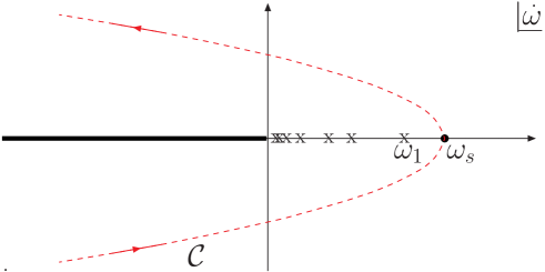
Figure 1: The $\omega$- plane and the contour of integration of eq.(3.1) for the case $\omega_{s}(t)\,>\,\omega_{1}$ . The x’s indicate the positions of the poles, which accumulate as $\omega\to 0$

The integrand in eq.(3.1) possesses a saddle point at $\omega=\omega_{s}$ in the $\omega$-plane, where $\omega_{s}$ is given by

$$\frac{d}{d\omega}\ln\left({\cal A}_{\omega}(t)\right)_{|\omega=\omega_{s}}\ =\ \ln(x)$$ (3.2)

where ${\cal A}_{\omega}(t)$ is defined by eq.(1.3). Provided this saddle point is also to the right of all singularities of ${\cal G}_{\omega}$, i.e. $\omega_{s}\,>\,\omega_{1}$, then the contour of integration can be deformed, as shown in Fig.1, so that it passes though the saddle point in the direction of steepest descent and the saddle-point approximation

$$\dot{g}(x,t)\ \approx\ \frac{1}{2\sqrt{\pi}\frac{d^{2}}{d\omega_{s}^{2}}\ln\left({\cal A}_{\omega_{s}}(t)\right)}x^{-\omega_{s}(t)}{\cal A}_{\omega_{s}}(t)$$ (3.3)

is a good approximation to the integral over $\omega$ in the Mellin inversion eq.(3.1).

For $t\,>\,t_{c}(\omega_{s})$, the amplitude ${\cal A}_{\omega_{s}}$ has a $t$-dependence

$${\cal A}_{\omega_{s}}(t)\ \sim\ \exp\left\{-\int^{t}\left|\nu_{\omega_{s}}(t^{\prime})\right|dt^{\prime}\right\}.$$ (3.4)

For sufficiently large $t$, the classical frequency, $\nu_{\omega_{s}}(t)$, is approximately given by

$$\left|\nu_{\omega_{s}}(t)\right|\ \stackrel{{\scriptstyle t\to\infty}}{{\rightarrow}}\ \frac{1}{2}-\frac{\bar{\alpha_{s}}(t)}{\omega_{s}}$$ (3.5)

and, as explained in refs. [11, 12, 8], in this limit the saddle-point $\omega_{s}$ coincides with the saddle-point obtained from inverting the gluon anomalous dimension, $\gamma^{N}_{gg}$ in the limit $N\,\to\,0$. Thus we obtain a match between the BFKL analysis and the $t$-dependence of a DGLAP analysis in the double logarithm limit, where both $t$ and $|\ln x|$ are large, namely (at leading order)

$${\cal A}_{\omega}(t)\ \stackrel{{\scriptstyle t\to\infty}}{{\sim}}\ e^{-t/2}\left(t\right)^{\frac{1}{\omega\bar{\beta_{0}}}}$$ (3.6)

In this case the $t$-dependence of the unintegrated gluon density (and consequently the $t$ dependence of the structure functions) is unaffected by the discrete nature of the BFKL spectrum.

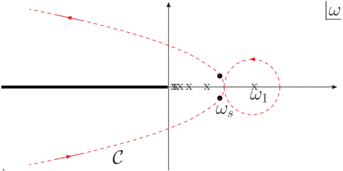
Figure 2: The $\omega$- plane and the contour of integration of eq.(3.1) for the case $\Re e\{\omega_{s}(t)\}\,<\,\omega_{1}$

On the other hand, if $t$ is not sufficiently large so that the (real part of the) saddle-point $\omega_{s}$ falls below one or more of the discrete eigenvalues $\omega_{n}$, then if one attempts to deform the contour so that it passes through the saddle-point (as shown in Fig.2 ) one has to surround one or more of the discrete poles of ${\cal G}_{\omega}$. In this case the contribution from the saddle-point given by eq.(3.3) has to be supplemented by the contribution from the contour surrounding the first $j$ discrete poles for which

$$\omega_{j+1}\ <\omega_{s}\ <\ \omega_{j},$$

i.e. we must add the contribution

$$\sum_{n=1}^{j}x^{-\omega_{n}}{\cal A}_{\omega_{n}}(t).$$

It is these extra terms that are sensitive to the heavy particle threshold behaviour of QCD and which give substantial deviations to the qualitative behaviour of the structure functions compared with the behaviour extracted from a purely DGLAP analysis. It is therefore important to emphasize that it is at relatively low values of $Q^{2}$ and small $x$ that we expect to see a signal of BFKL dynamics which can be clearly distinguished from the predictions of DGLAP.

4 Summary

In this paper, we have analyzed the (Mellin transform of the) Green function for the BFKL amplitude in the semi-classical approximation in which it can be cast into the form of the Green function of Airy’s equation after a suitable change of variables. The general solution contains terms with poles for positive $\omega$ as well as an analytic part constructed from the two independent solutions to Airy’s equation. Our expression for the Green function differs from that previously obtained in refs.[1, 2, 3] in that in addition to the component consisting of a set of discrete poles in the Mellin transform variable, $\omega$, there is a component which is analytic in $\omega$. This latter part turns out to be necessary in order to generate a match to the result of a DGLAP analysis in the DLL limit. We have obtained an approximate expression for the unintegrated gluon density by considering the saddle-point approximation to the inverse Mellin transform. For sufficiently large values of transverse momentum the saddle-point lies to the right of all the poles and the match with the result of a DGLAP analysis in the DLL limit follows in the same way as the case of the continuum BFKL pomeron. However, as the gluon transverse momentum becomes small, the saddle-point lies to the left of some of the discrete poles and in such cases the unintegrated gluon density is supplemented by the contribution from the integral around these poles.

A complete numerical analysis, which does not rely on the saddle-point approximation, following the programme described in this paper is currently under way and will be published in a forthcoming paper.

References

- [1] J. Ellis, H. Kowalski and D. A. Ross, Phys. Lett. B 668 (2008) 51.
-
[2]
H. Kowalski, L.N. Lipatov, D. A. Ross, and G. Watt
Eur. Phys. J C70 (2010) 983;
Nucl. Phys A854 (2011) 45 - [3] H. Kowalski, L.N. Lipatov,and D. A. Ross, Phys. Part. Nucl. 44 (2013) 547
- [4] I. I. Balitsky and L. N. Lipatov, Sov. J. Nucl. Phys. 28 (1978) 822; E. A. Kuraev, L. N. Lipatov and V. S. Fadin, Sov. Phys. JETP 44 (1976) 443; V. S. Fadin, E. A. Kuraev and L. N. Lipatov, Phys. Lett. B 60 (1975) 50.
- [5] L. N. Lipatov, Sov. Phys. JETP 63 (1986) 904.
-
[6]
V.N. Gribov and L.N. Lipatov, Sov. Nucl. Phys. 15 (1972) 438
G. Altarelli and G. Parisi, Nucl. Phys. B126 (1977) 298
Yu. L. Dokshitzer, Sov. Phys. JETP 46 (1977) 46
-
[7]
M. Ciafaloni and D. Colferai, Phys. Lett. B452 (1999) 372
M. Ciafaloni, D. Colferai and D.P. Salam, Phys. Rev. D60 (1999) 114036
M. Ciafaloni, D. Colferai, D.P. Salam and A. Stasto, Phys. Rev. D66 (2002) 054014 -
[8]
Altarelli, Ball, Forte
G. Altarelli, R.Ball and S.Forte, Nucl. Phys., B621 (2002) 359
G. Altarelli, R.Ball and S.Forte, Nucl. Phys., B674 (2003) 459
G. Altarelli, R.Ball and S.Forte, Nucl. Phys., B743 (2006) 1 - [9] G. P. Salam, JHEP 9807 (1998) 019.
- [10] V. S. Fadin and L. N. Lipatov, Phys. Lett. B 429 (1998) 127; M. Ciafaloni and G. Camici, Phys. Lett. B 430 (1998) 349.
-
[11]
M. Ciafaloni and D. Colferai, Phys. Lett. B452 (1999) 372
M. Ciafaloni, D. Colferai and D.P. Salam, Phys. Rev. D60 (1999) 114036
M. Ciafaloni, D. Colferai, D.P. Salam and A. Stasto, Phys. Rev. D66 (2002) 054014 - [12] R.S. Thorne and C.D. White, Phys. Rev. D75 (2007) 034005