Finite-Time-Finite-Size Scaling of the Kuramoto Oscillators

Abstract

We numerically investigate the short-time nonequilibrium temporal relaxation of the globally-coupled Kuramoto oscillators, and apply the finite-time-finite-size scaling (FTFSS) method which contains two scaling variables in contrast to the conventional single-variable finite-size scaling. The FTFSS method yields a smooth scaling surface, and the conventional finite-size scaling curves can be viewed as proper cross sections of the surface. The validity of our FTFSS method is confirmed by the critical exponents in agreement with previous studies: Quenched disorder gives the correlation exponent $\bar{\nu}=5/2$ and the dynamic exponent $\bar{z}=2/5$ while thermal disorder leads to $\bar{\nu}=2$ and $\bar{z}=1/2$, respectively. We also report our results for the Kuramoto model in the presence of both quenched and thermal disorder.

In the frame of statistical physics, it is important to find critical exponents in a system aiming at understanding of its critical behaviors. For a limited number of model systems, it might be possible to analytically obtain the exponents via the mean-field analysis, transfer-matrix calculation, the renormalization group approach, and other analytic tools golden . In most of realistic model systems, however, a rigorous analytic calculation of critical exponents is often a formidable task, making numerical approaches unavoidable and essential.

A phase transition manifests itself as a singularity of the free energy, which exists only in thermodynamic limit of the infinite system size. On the other hand, one can only simulate finite systems in any computational approach, which results in the so-called finite-size effects. The very finiteness of system sizes can be utilized in the form of the finite-size scaling (FSS), which has been successfully used to extract critical exponents privman . In the conventional FSS, the system under study is asked to be in equilibrium, and thus the functional form of FSS lacks any time dependence. As the system size becomes larger, the time scale at criticality often diverges together with the correlation length, which gives rise to the critical slowing down. In order to circumvent this, the finite-size dynamical scaling approach zheng ; soares has been introduced. The basic assumption in this approach of dynamical scaling is that one can extract critical behavior by observing the temporal relaxation of the system in early times even before reaching equilibrium.

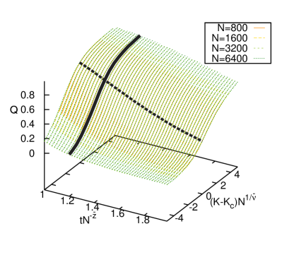
Figure 1: (Color online) Finite-time-finite-size scaling (FTFSS): $Q(t,N,K)=f\Bigl{(}tN^{\bar{z}},(K-K_{c})N^{1/\bar{\nu}}\Bigr{)}$ for the globally-coupled Kuramoto oscillators with quenched disorder yields a smooth scaling surface with $\bar{\nu}=5/2$, $\bar{z}=2/5$, and $K_{c}=1.595769$. The scaling collapse is good enough to make difference of surfaces obtained from different sizes $N=800,1600,3200$, and 6400 almost invisible. The thick dashed and solid lines are two cross sections of the surface at $tN^{-\bar{z}}=1.2$ and at $K=K_{c}$ displayed in Fig. 2(b) and (d), respectively.

In general, one can assume that a time-varying thermodynamic quantity $Q$ is a function of the time $t$, the linear size $L$, and the coupling strength $K$. As the critical point $K=K_{c}$ is approached, the correlation length $\xi$ diverges following the form $\xi\sim(K-K_{c})^{-\nu}$ and so does the relaxation time scale $\tau\sim\xi^{z}$. If we further assume that $Q$ is chosen in such a way that its anomalous dimension is null soares , the scaling form of $Q$ is written as $Q(t,L,K)=f\Bigl{(}tL^{-z},(K-K_{c})L^{1/\nu}\Bigr{)}$. In words, the first scaling variable $tL^{-z}$ describes the competition of the two time scales, the finite observation time $t$ and the relaxation time $\tau$, while the second scaling variable $(K-K_{c})L^{1/\nu}$ is for the competition of the two length scales, the finite system size $L$ and the correlation length $\xi$. It is straightforward to extend the scaling form for the globally-coupled system, which reads

$$Q(t,N,K)=f\Bigl{(}tN^{-\bar{z}},(K-K_{c})N^{1/\bar{\nu}}\Bigr{)},$$ (1)

where $N$ is the size of the system and $\bar{\nu}$ and $\bar{z}$ are correlation and dynamic exponents defined for globally-coupled system. Throughout the present study, we term the scaling in Eq. (1) as finite-time-finite-size scaling (FTFSS). Precisely speaking, the phase transition is defined only in the limit of infinite time $t\rightarrow\infty$ and infinite system size $N\rightarrow\infty$, whereas any numerical calculation is limited by finiteness of $t$ and $N$. Just like the conventional FSS aims to systematically utilizes the finite-size effect by using the scaling variable $L/\xi$, our FTFSS uses $t/\tau$ as well to utilize the finite-time effect introduced by the finiteness of the observation time $t$. Figure 1 exhibits how the FTFSS can be used to produce a smooth scaling surface for the globally-coupled Kuramoto model (see below for details).

Model – Synchronization phenomena are ubiquitously observed in a variety of systems such as the neuronal network and epilepsy in the brain epilepsy ; undesired , circadian rhythm circadian , the collapse of the Millennium Bridge bridge , power grids powergrid0 ; powergrid , and social behavior of humans heavymetal . Kuramoto model has been most popularly used to describe such synchronization phenomena, and we study the globally-coupled $N$ oscillators with both quenched intrinsic frequency $\omega_{i}$ and thermal noise $\eta_{i}$ described by

$$\frac{d\theta_{i}}{dt}=\omega_{i}-\frac{K}{N}\sum_{j=1}^{N}\sin(\theta_{i}-\theta_{j})+\eta_{i}(t),$$ (2)

where $K$ is the coupling strength and $\theta_{i}$ is the phase of the $i$-th oscillator. We use the Gaussian distribution of the zero mean and the variance $\sigma^{2}$ for the distribution function for $\omega_{i}$, and the thermal noise satisfies $\langle\eta_{i}\rangle=0$ and $\langle\eta_{i}(t)\eta_{j}(t^{\prime})\rangle=2T\delta_{ij}\delta(t-t^{\prime})$ with $T$ being the effective temperature and $\langle\cdots\rangle$ the ensemble average. In the zero-temperature limit of $T\rightarrow 0$, the system corresponds to the conventional Kuramoto model for which the correlation exponent $\bar{\nu}=5/2$ hong2007 ; mha and the dynamic exponent $\bar{z}=2/5$ mha have been found. In the limit of $\sigma\rightarrow 0$, on the other hand, the system behaves as the globally-coupled $XY$ model for which $\bar{\nu}=2$ son2010 ; mha and $\bar{z}=1/2$ mha are known. This equation of motion (2) in a finite dimension can be viewed as the time-dependent Ginzberg Landau (TDGL) dynamics of the superconducting array with the dc current $\omega_{i}$ and the thermal noise current $\eta_{i}$ kimTDGL .

In order to carry out FTFSS, we use the initial condition $\theta_{i}(t=0)=0$ for all oscillators and measure the key quantity $Q(t)$ defined by kim3dxy ; melwyn4dxy

$$Q(t)\equiv\left\langle\textrm{sign}\left[\sum_{i=1}^{N}\cos\theta_{i}(t)\right]\right\rangle,$$ (3)

which satisfies $Q(0)=1$ and $Q(t\rightarrow\infty)=0$ at any parameter values of $K$, $\sigma$, and $T$ due to the rotational $U(1)$ symmetry in equilibrium. The advantage of using $Q$ lies on that it does not have the anomalous dimension soares , which allows us to use the simple FTFSS form in Eq. (1). We also emphasize that our FTFSS method uses how $Q(t)$ evolves in time before reaching equilibrium, and thus equilibration is not a requirement to extract critical exponents zheng . However, it is to be noted that before the ensemble average $\langle\cdots\rangle$, each sample run returns the value either $+1$ or $-1$ at time $t$ since only the sign is taken in Eq. (3). This means that in order to get a smooth continuous form for $Q(t)$ as a function of time $t$, the ensemble average must be performed over sufficiently many samples. We use the second-order algorithm to integrate equation of motion with the discrete time step $\Delta t=0.01$.

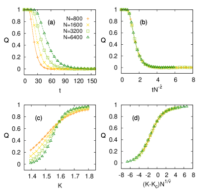
Figure 2: (Color online) The two-variable FTFSS form (1) in Fig. 1 at zero temperature is cross sectioned to one variable scaling form (b) $Q=f\bigl{(}tN^{-\bar{z}},0\bigr{)}$ at $K=K_{c}$ and (d) $Q=f(tN^{-\bar{z}}=1.2,(K-K_{c})N^{1/\bar{\nu}})$. The raw data [(a) and (c)] obtained for various system sizes are scaled into smooth scaling curves [(b) and (d)] with the critical exponents (b) $\bar{z}=2/5$ and (d) $\bar{\nu}=5/2$ with the critical coupling strength $K_{c}=1.595769$.

Results – We first report the scaling results obtained from 100000 samples for the usual Kuramoto model with only the quenched randomness in the intrinsic frequency, corresponding to the zero-temperature limit of Eq. (2). The full FTFSS with the two scaling variables in Eq. (1) is shown in Fig. 1 with $\sigma=1$. All surfaces obtained for various sizes $N=800,1600,3200$, and 6400 collapse into a single smooth surface with the critical exponents $\bar{\nu}=5/2$, $\bar{z}=2/5$ and the critical coupling strength $K_{c}=\sqrt{8/\pi}=1.595769$, as expected from previous studies son2010 ; mha . The dynamic scaling mha is easily obtained by fixing the second scaling variable in the FTFSS (1) to null by putting $K=K_{c}$ as shown in Fig. 2(b). All the curves in Fig. 2(a) are shown to collapse nicely into a single smooth curve. Interesting application of the FTFSS is achieved by fixing the first scaling variable $tN^{-\bar{z}}$ in Eq. (1), to make the FTFSS form identical to the conventional FSS form. As an example, we use $\alpha\equiv tN^{-\bar{z}}=1.2$ to plot Fig. 2(d). It is clearly seen that by fixing the first scaling variable, one can successfully obtain the critical exponent $\bar{\nu}=5/2$ and $K_{c}=1.595769$. In order to get such a finite-size scaling as in Fig. 2(d), it is important to choose the observation time $t$ systematically for the given system size $N$ to keep the value $tN^{-\bar{z}}$ as constant.

In other extreme case with only thermal noise, corresponding to $\sigma=0$ in Eq. (2), the dynamics is effectively identical to the mean-field version of the TDGL equation, for which it is known that $\bar{\nu}=\nu d_{u}=2$ and $\bar{z}=z/d_{u}=1/2$ beyond upper critical dimension $d_{u}=4$ melwyn4dxy . In parallel to Fig. 2 where $K$ is in units of $\sigma$, we now measure $K$ in units of the temperature $T$. From the well-known result that the critical value of $T/K$ is 1/2 for the globally-coupled $XY$ model globalXY , we expect that $K_{c}=2$ in units of the temperature $T$. In the presence of thermal noise, integration of equation of motion takes much longer time since generation of random number is needed at each time step. We use $N=400$, 800, and 1600 and the ensemble averages are performed for 20000 samples. As expected from known results of $K_{c}=2$, $\bar{\nu}=2$, and $\bar{z}=1/2$, our FTFSS gives us again a good quality of scaling surface as shown in Fig. 3(a). As in Fig. 2, we also make cross sections of the scaling surface to construct scaling collapses in Fig. 3(b) and (c), in which it is shown clearly that the use of $\bar{\nu}=2$ and $\bar{z}=1/2$ with $K_{c}=2$ yields scaling collapses as expected.

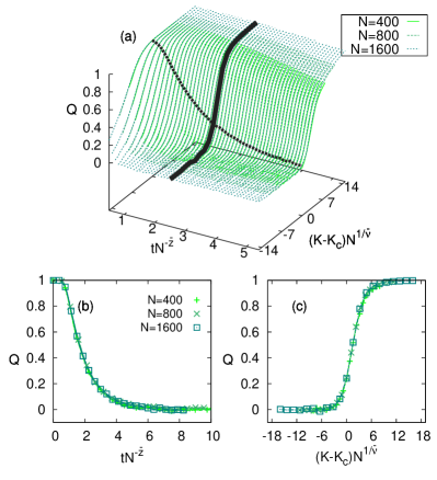
Figure 3: (Color online) FTFSS for the globally-coupled Kuramoto oscillators with thermal disorder only: $\bar{\nu}=2$ and $\bar{z}=1/2$ are obtained at $K_{c}=2$ (in units of the temperature $T$). The thick dashed and solid lines are two cross sections of the surface at $tN^{-\bar{z}}=2.5$ and at $K=K_{c}$ displayed in (b) and (c), respectively.

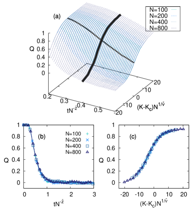
Figure 4: (Color online) FTFSS for the globally-coupled Kuramoto oscillators with both disorders: $\bar{\nu}=2.22$ and $\bar{z}=0.45$ are obtained at $K_{c}=5$ with $\sigma=2.28006$ (in units of the temperature $T$). The thick dashed and solid lines are two cross sections of the surface at $tN^{-\bar{z}}=0.4$ and at $K=K_{c}$ displayed in (b) and (c), respectively.

Table 1: The correlation exponent $\bar{\nu}$ is computed along the phase boundary in the $(T,\sigma)$ plane (see Fig. 1 of son2010 ) via the FTFSS of $Q$ and the FSS of $r$. The system sizes used here are 100, 200, 400, and 800 with 10000 samples. Estimation through the use of $Q$ gives us more accurate values of $\bar{\nu}=5/2$ and $\bar{z}=2$ at $T=0$ and $T=0.5$, respectively. We also include the value of $\bar{z}$ from the FTFSS of $Q$, which satisfies $\bar{z}\approx 1/\bar{\nu}$.

$T/K$	$\bar{\nu}$ from $r$	$\bar{\nu}$ from $Q$	$\bar{z}$ from $Q$
$0$	$2.35$	$2.5$	$0.4$
$0.1$	$2.23$	$2.38$	$0.42$
$0.2$	$2.11$	$2.22$	$0.45$
$0.3$	$2.07$	$2.08$	$0.48$
$0.4$	$2.03$	$2.04$	$0.49$
$0.5$	$1.98$	$2$	$0.5$

Motivated by the success of our FTFSS method for the Kuramoto model in the presence of either purely quenched disorder (Figs. 1 and 2) or purely thermal disorder (Fig. 3), we next study the Kuramoto systems with both types of disorder ($\sigma\neq 0$ and $T\neq 0$). In Fig. 4, we show the FTFSS of $Q$ at $\sigma/T=2.28006$ gives us a good quality of scaling collapse with $\bar{\nu}=2.22$, $\bar{z}=0.45$, and $K_{c}/T=5$ (the values for $\sigma/T$ and $K_{c}/T$ are taken on the phase boundary in son2010 ). It has been suggested that the upper critical dimension $d_{u}=5$ for the Kuramoto model with quenched randomness hong2005 , and $d_{u}=4$ has been agreed for the globally-coupled $XY$ model globalXY , which explains the values obtained above ($\bar{\nu}=5/2,\bar{z}=2/5$ for quenched, and $\bar{\nu}=2,\bar{z}=1/2$ for thermal disorder, respectively) on equal footing via $\bar{\nu}=\nu d_{u}$ and $\bar{z}=z/d_{u}$ with $\nu=1/2$ and $z=2$. The phase diagram in the two-dimensional parameter space of $(T,\sigma)$ with both in units of $K$ has been obtained in son2010 . We apply the FTFSS for our key quantity $Q$ in the same way as above to find the critical exponents along the phase boundary, and compare with the results obtained from the standard finite-size scaling of the Kuramoto order parameter $r$ defined by

$$r\equiv\left\langle\left|\frac{1}{N}\sum_{i}e^{i\theta}\right|\right\rangle,$$ (4)

where $\langle\cdots\rangle$ is for both the sample average and the temporal average after equilibration. The standard FSS form $r=N^{-\beta/\bar{\nu}}g\bigl{(}(T-T_{c})N^{1/\bar{\nu}}\bigr{)}$ is then used with the critical exponent $\beta=1/2$ son2010 for the order parameter. In Table 1 we compare $\bar{\nu}$ obtained from the FTFSS of $Q$ and from the FSS of $r$, along the phase boundary presented in Fig. 1 of son2010 . In the zero-temperature limit, the correct value $\bar{\nu}=5/2$ is well obtained from $Q$, but the value is rather inaccurate if $r$ is used instead. In other limit of $\sigma=0$ for which the phase boundary crosses $T$ axis at 1/2, the value $\bar{\nu}\approx 2$ from $Q$ is more accurate than the one from $r$ although the difference is not as significant as in the zero-temperature case. Another advantage of the FTFSS of $Q$ is that it allows us to obtain other exponent $\bar{z}$, which is also listed in Table 1. It is noteworthy that along the full phase boundary, $\bar{z}=1/\bar{\nu}$ is found regardless of the value of $T/K$, which appears to suggest that $\bar{z}\bar{\nu}=(z/d_{u})(\nu d_{u})=z\nu=2\cdot(1/2)=1$ remains constant along the phase boundary. Standard universality argument suggests that as soon as thermal disorder is added to the Kuramoto system $\bar{\nu}$ is expected to change abruptly from 5/2 to 2. Although our results in Table 1 do not show such an abrupt change of $\bar{\nu}$, we believe that this can be an finite-size artifact which might disappear if much bigger system sizes are used. In spite of the advantage of using the FTFSS of $Q$ that only initial stage of nonequilibrium short-time relaxation is enough to detect universality class, we point out that the calculation of $Q$ requires average over a larger number of samples. In contrast, the calculation of $r$, for large systems in particular, does not require extensive sample average, thanks to the self-averaging property.

Conclusion and Summary – We have applied the finite-time-finite-size scaling (FTFSS) for the globally-coupled Kuramoto model with quenched and thermal disorders. The key quantity $Q(t)$ has been defined as the ensemble average of the sign of the real part of the Kuramoto order parameter, and measured as a function of time $t$. We have found that the FTFSS with the two scaling variables yields a well-defined scaling surface, cross sections of which in two different directions lead to the standard finite-size scaling as well as the dynamic scaling. Correlation critical exponent $\bar{\nu}$ and the dynamic critical exponent $\bar{z}$ have been obtained through the use of FTFSS applied for the quantity $Q(t)$, confirming the results from previous studies: $\bar{\nu}=5/2,\bar{z}=2/5$ for purely quenched randomness and $\bar{\nu}=2,\bar{z}=1/2$ for purely thermal noise. Our FTFSS of $Q(t)$ is based on the early stage of nonequilibrium relaxation and thus makes it possible to avoid the critical slowing down near the criticality.

This work was supported by the National Research Foundation of Korea (NRF) grant funded by the Korea government (MEST) (No. 2011-0015731).

References

- (1) N. Goldenfeld, Lectures on Phase Transitions and the Renormalization Group, (Addison-Wesley, New York, 1992)
- (2) D. Privman, Finite Size Scaling and Numerical Simulation of Statistical Systems, (World Scientific, Singapore, 1990).
- (3) Z. B. Li, L. Schülke, and B. Zheng, Phys. Rev. Lett. 74, 3396 (1995).
- (4) M. S. Soares, J. K. L. da Silva, F. C. S. Barreto, Phys. Rev. B 55, 1021 (1997).
- (5) C. Choi, M. Ha, and B. Kahng, arXiv:1307.2408v1 (2013).
- (6) R. S. Fisher, W. v. E. Boas, W. Blume, C. Elger, P. Genton, P. Lee, and J. Engel, Epilepsia 46, 470 (2005).
- (7) V. H. P. Louzada, N. A. M. Araújo, J. S. Andrade Jr., and H. J. Herrmann, Sci. Rep. 2, 658 (2012).
- (8) E. Kolmos and S. J. Davis, Current Biology, 17(18), 808 (2007).
- (9) S. H. Strogatz, D. M. Abrams, A. McRobie, B. Eckhardt, and E. Ott, Nature, 438, 43. (2005).
- (10) G. Filatrella, A. H. Nielsen, and N. F. Pedersen, Eur. Phys. J. B 61, 485 (2008).
- (11) M. Rohden, A. Sorge, M. Timme, and D. Witthaut, Phys. Rev. Lett. 109, 064101 (2012).
- (12) J. L. Silverberg, M. Bierbaum, J. P. Sethna, and I. Cohen, Phys. Rev. Lett. 110, 228701 (2013).
- (13) H. Hong, H. Chaté, H. Park, and L.-H Tang, Phys. Rev. Lett. 99, 184101 (2007).
- (14) S.-W. Son and H. Hong, Phys. Rev. E 81, 061125 (2010).
- (15) B. J. Kim, P. Minnhagen, and P. Olsson, Phys. Rev. B 59, 11506 (1999).
- (16) B. J. Kim, L. M. Jensen, and P. Minnhagen, Physica B 284, 413 (2000).
- (17) L. M. Jensen, B. J. Kim, and P. Minnhagen, Physica B 284, 455 (2000).
- (18) S. K. Baek and B. J. Kim, Phys. Rev. E 86, 011132 (2012); B. J. Kim, H. Hong, P. Holme, G. S. Jeon, P. Minnhagen, and M. Y. Choi, Phys. Rev. E 64, 056135 (2001); M. Antoni and S. Ruffo, Phys. Rev. B 52, 2361 (1995).
- (19) H. Hong, H. Park, and M. Y. Choi, Phys. Rev. E 72, 036217 (2005).