Band Tunneling through Double Barrier in Bilayer Graphene

Hasan A. Alshehab^a,b, Hocine Bahlouli^a,b, Abderrahim El Mouhafid^c and Ahmed Jellal^b,c

^aPhysics Department, King Fahd University of Petroleum $\&$ Minerals,
Dhahran 31261, Saudi Arabia

^bSaudi Center for Theoretical Physics, Dhahran, Saudi Arabia

^cTheoretical Physics Group, Faculty of Sciences, Chouaïb Doukkali University,

PO Box 20, 24000 El Jadida, Morocco

By taking into account the full four band energy spectrum, we calculate the transmission probability and conductance of electrons across symmetric and asymmetric double potential barrier with a confined interlayer potential difference in bilayer graphene. For energies less than the interlayer coupling $\gamma_{1}$, $E<\gamma_{1}$, we have one channel for transmission which exhibits resonances, even for incident particles with energies less than the strength of barriers, $E<U_{j}$, depending on the double barrier geometry. In contrast, for higher energies $E>\gamma_{1}$, we obtain four possible ways for transmission resulting from the two propagating modes. We compute the associated transmission probabilities as well as their contribution to the conductance, study the effect of the double barrier geometry.

PACS numbers: 73.22.Pr; 73.63.-b; 72.80.Vp

Keywords: bilayer graphene, double barrier, transmission, conductance.

1 Introduction

In the last few years, graphene [1], a two dimensional one atom thick sheet of carbon, became a hot research topic in the field of condensed matter physics. Its exceptional, electronic, optical, thermal, and mechanical properties have potential future applications. For example, its thermal conductivity is 15 times larger than that of copper and its electron mobility is 20 times larger than that of GaAs. In addition, it is considered as one of the strongest materials with a Young’s modulus of about 1 TPa, and some 200 times stronger than structural steel[2]. The most important application of graphene is to possibly replace silicon in IT-technology. But the biggest obstacle is to create a gap and control the electron mobility in graphene taking into account the so called Klein tunneling, which makes the task more complicated[3, 4]. However, one can create an energy gap in the spectrum in many different ways, such as by coupling to substrate or doping with impurities [5, 6] or in bilayer graphene by applying an external electric field [7, 8].

Bilayer graphene is two stacked (Bernal stacking [9]) monolayer graphene sheets, each with honeycomb crystal structure, with four atoms in the unit cell, two in each layer. In the first Brillouin zone, the tight binding model for bilayer graphene [10] predicted four bands, two conduction bands and two valance bands, each pair is separated by an interlayer coupling energy of order $\gamma_{1}\approx 0.4\ eV$ [11]. At the Dirac points, one valance band and one conduction band touch at zero energy, whereas the other bands are split away from the zero energy by $\gamma_{1}$ [12]. Further details about band structure and electronic properties of bilayer graphene can be found in the literature [13, 14, 15, 16, 17, 18, 19, 20, 21]. Tunneling of quasiparticles in graphene, which mimics relativistic quantum particles such as Dirac fermions in quantum electrodynamics (QED), plays a major role in scattering theory. It allows to develop a theoretical framework, which leads to investigate different physical phenomena that are not present in the non relativistic regime, such as the Klein-paradox [3, 4].

In monolayer graphene, there were many studies on the tunneling of electrons through different potential shapes [22, 23, 24, 25]. While the study of tunneling electrons in bilayer graphene has been restricted to energies less than the interlayer coupling parameter $\gamma_{1}$ so that only one channel dominates transmission and the two band model is valid [26, 27, 28, 29]. Recently, tunneling of electrons in bilayer graphene has been studied using the four band model for a wide range of energies, even for energies larger than $\gamma_{1}$ [30]. New transmission resonances were found that appear as sharp peaks in the conductance, which are absent in the two band approximation.

Motivated by different developments and in particular [30], we investigate the band tunneling through square double barrier in bilayer graphene. More precisely, the transmission probabilities and conductance of electrons will be studied by tacking into account the full four band energy spectrum. We analyze two interesting cases by making comparison between the incident energies $E$ and interlayer coupling parameter $\gamma_{1}$. Indeed, for $E<\gamma_{1}$ there is only one channel of transmission exhibiting resonances, even for incident particles with $E$ less than the strength of barriers $U_{j}$ ($E<U_{j}$), depending on the double barrier geometry. For $E>\gamma_{1}$, we end up with two propagating modes resulting from four possible ways of transmission. Subsequently, we use the transfer matrix and density of current to determine the transmission probabilities and then the corresponding conductance. Based on the physical parameters of our system, we present different numerical results and make comparison with significant published works on the subject.

The present paper is organized as follows. In section 2, we establish a theoretical framework using the four band model leading to four coupled differential equations. In section 3, by using the transfer matrix at boundaries together with the incident, transmitted and reflected currents we end up with eight transmission and reflection probabilities as well as the corresponding conductance. We deal with two band tunneling and analyze their features with and without the interlayer potential difference, in section 4. We do the same job in section 5 but by considering four band energy and underline the difference with respect to other case. In section 6, we show the numerical results for the conductance and investigate the contribution of each transmission channel. Finally, we briefly summarize our main findings in the last section.

2 Theoretical model

In monolayer graphene, the unit cell has inequivalent atoms (usually called A and B). Bilayer graphene on the other hand is a two stacked monolayer graphene (Bernal stacking) and hence has four atoms in the unit cell. The relevant Hamiltonian near the $K$ point (the boundary of the Brillouin zone), can be found using the nearest-neighbor tight binding approximation[17]

$$H=\left(\begin{array}[]{cccc}V^{+}&v_{F}\pi^{{\dagger}}&-v_{4}\pi^{{\dagger}}&v_{3}\pi\\ v_{F}\pi&V^{+}&\gamma_{1}&-v_{4}\pi^{{\dagger}}\\ -v_{4}\pi&\gamma_{1}&V^{-}&v_{F}\pi^{{\dagger}}\\ v_{3}\pi^{{\dagger}}&-v_{4}\pi&v_{F}\pi&V^{-}\\ \end{array}\right)$$ (1)

where $v_{F}=\frac{\gamma_{0}}{\hbar}\frac{3a}{2}\approx 10^{6}\ {m}/{s}$ is the fermi velocity of electrons in each graphene layer, $a=0.142\ nm$ is the distance between adjacent carbon atoms, $v_{3,4}=\frac{v_{F}\gamma_{3,4}}{\gamma_{0}}$ represent the coupling between the layers, $\pi=p_{x}+ip_{y},\pi^{{\dagger}}=p_{x}-ip_{y}$ are the in-plan momenta and its conjugate with $p_{x,y}=-i\hbar\partial_{x,y}$. $\gamma_{1}\approx 0.4\ eV$ is the interlayer coupling term and $V^{+},V^{-}$ are the potentials on the first and second layer, respectively. The skew parameters , $\gamma_{3}\approx 0.315\ eV$ and $\gamma_{4}\approx 0.044\ eV$ have negligible effect on the band structure at high energy[12, 13]. Recently, it was shown that even at low energy these parameters have also negligible effect on the transmission[30], hence we neglect them in our calculations.

Under the above approximation and for double barrier potential configuration in Figure 1

Figure 1: The parameters of a rectangular double barrier structure.

our previous Hamiltonian (1) can be written as follows in each potential region where we define regions as follows: $j=1$ for $x\leq a$, $j=2$ for $a<x\leq b$, $j=3$ for $b<x\leq c$, $j=4$ for $c<x\leq d$ and $j=5$ for $x>d$ so that in the $j$-th region we have

$$H_{j}=\left(\begin{array}[]{cccc}V^{+}_{j}&\nu_{F}\pi^{{\dagger}}&0&0\\ \nu_{F}\pi&V^{+}_{j}&\gamma_{1}&0\\ 0&\gamma_{1}&V^{-}_{j}&\nu_{F}\pi^{{\dagger}}\\ 0&0&\nu_{F}\pi&V^{-}_{j}\\ \end{array}\right)$$ (2)

We define the potential on the first and second layer by $V^{\pm}_{j}=U_{j}\pm\delta_{j}$, where $U_{j}$ is the barrier strength and $\delta_{j}$ is the electrostatic potential in the $j$-th region

$$V^{\pm}_{j}=\left\{\begin{array}[]{lllll}0,&\qquad\hbox{$j=1$}\\ U_{2}\pm\delta_{2},&\qquad\hbox{$j=2$}\\ 0,&\qquad\hbox{$j=3$}\\ U_{4}\pm\delta_{4},&\qquad\hbox{$j=4$}\\ 0,&\qquad\hbox{$j=5$}\\ \end{array}\right.$$ (3)

($U_{2},\delta_{2}$) and ($U_{4},\delta_{4}$) are the barrier potential and the electrostatic potential in regions 2 and 4, respectively.

The eigenstates of (2) are four-components spinors $\psi^{j}(x,y)=[{\psi}^{j}_{A_{1}},{\psi}^{j}_{B_{1}},{\psi}^{j}_{A_{2}},{\psi}^{j}_{B_{2}}]^{{\dagger}}$, here ${\dagger}$ denotes the transpose of the row vector. For a double barrier we need to obtain the solution in each regions as shown in Figure 1. Since we have basically two different sectors with zero (1, 3, 5) and nonzero potential (2, 4), a general solution can be obtained in the second sector and then set the potential $V^{\pm}_{j}$ to zero to obtain the solution in the first sector. To simplify the notation, let us introduce the length scale $l=\frac{\hbar v_{F}}{\gamma_{1}}\approx 1.76\ nm$ as well as $E_{j}\longrightarrow\frac{E}{\gamma_{1}}$ and $V_{j}\longrightarrow\frac{V_{j}}{\gamma_{1}}$. Since the momentum along the $y$-direction is a conserved quantity, i.e $[H,p_{y}]=0$, and therefore we can write the spinors as

$$\psi^{j}(x,y)=e^{ik_{y}y}[{\phi}^{j}_{A_{1}},{\phi}^{j}_{B_{1}},{\phi}^{j}_{A_{2}},{\phi}^{j}_{B_{2}}]^{T}$$ (4)

As usual, to derive the eigenvalues and the eingespinors we solve $H_{j}\psi_{j}=E_{j}\psi_{j}$. Then, by replacing by (2) and (4) we obtain

$$\left(\begin{array}[]{cccc}U_{j}+\delta_{j}&\frac{l}{\hbar}\pi^{{\dagger}}&0&0\\ \frac{l}{\hbar}\pi&U_{j}+\delta_{j}&1&0\\ 0&1&U_{j}-\delta_{j}&\frac{l}{\hbar}\pi^{{\dagger}}\\ 0&0&\frac{l}{\hbar}\pi&U_{j}-\delta_{j}\\ \end{array}\right)\ \left(\begin{array}[]{c}\phi^{j}_{A_{1}}\\ \phi^{j}_{B_{1}}\\ \phi^{j}_{A_{2}}\\ \phi^{j}_{B_{2}}\\ \end{array}\right)e^{iky}=E_{j}\left(\begin{array}[]{c}\phi^{j}_{A_{1}}\\ \phi^{j}_{B_{1}}\\ \phi^{j}_{A_{2}}\\ \phi^{j}_{B_{2}}\\ \end{array}\right)e^{iky}$$ (5)

This gives four coupled differential equations

$$-il\left[\frac{d}{dx}+ky\right]\phi^{j}_{B1}=(\epsilon_{j}-\delta_{j})\phi^{j}_{A1}$$ (6)

$$-il\left[\frac{d}{dx}-ky\right]\phi^{j}_{A1}+\phi^{j}_{A2}=(\epsilon_{j}-\delta_{j})\phi^{j}_{B1}$$ (7)

$$-il\left[\frac{d}{dx}+ky\right]\phi^{j}_{B2}+\phi^{j}_{B1}=(\epsilon_{j}+\delta_{j})\phi^{j}_{A2}$$ (8)

$$-il\left[\frac{d}{dx}-ky\right]\phi^{j}_{A2}=(\epsilon_{j}+\delta_{j})\phi^{j}_{B2}$$ (9)

where $k_{y}$ is the wave vector along the $y$-direction and we have set $\epsilon_{j}=E_{j}-U_{j}$. It is easy to decouple the first equations to obtain

$$\left[\frac{d^{2}}{dx^{2}}+(k^{s}_{j})^{2}\right]\phi^{j}_{B1}=0$$ (10)

where the wave vector along the $x$-direction is

$$k^{s}_{j}=\left[-k^{2}_{y}+\frac{\epsilon^{2}_{j}+(\delta_{j})^{2}}{l^{2}}+s\frac{1}{l^{2}}\sqrt{\epsilon^{2}_{j}(1+4(\delta_{j})^{2})-(\delta_{j})^{2}}\right]^{1/2}$$ (11)

where $s=\pm$ denotes the propagating modes which will be discussed latter on. Now for each region one can end up with corresponding wave vector according to Figure 1. Indeed, for regions 1, 3 and 5 we have $V^{\pm}_{j}=0$ and then we can obtain

$$k^{s}_{0}=\left[-k^{2}_{y}+\frac{\epsilon^{2}}{l^{2}}+s\frac{\epsilon}{l^{2}}\right]^{1/2}$$ (12)

with $\epsilon=\epsilon_{1}=\epsilon_{3}=\epsilon_{5}$, as well as the energy

$$E^{s}_{\pm}=\pm\frac{1}{2}\left[-s+\sqrt{1+(2lk_{0}^{s})^{2}+(2lk_{y})^{2}}\right]$$ (13)

However generally, for any region we can deduce energy from previous analysis as

$$\epsilon^{s}_{\pm,j}=\pm\frac{1}{\sqrt{2}}\left[1+2l^{2}\left[(k_{j}^{s})^{2}+k_{y}^{2}\right]+2\delta_{j}^{2}-s\sqrt{1+4l^{2}\left[(k_{j}^{s})^{2}+k_{y}^{2}\right]\left(1+4\delta_{j}^{2}\right)}\right]^{1/2}.$$ (14)

The corresponding energy spectrum of the different regions is shown in Figure 2.

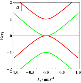
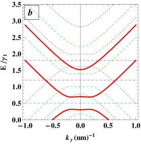
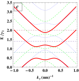
Figure 2: Energy as function of the momentum $k_{y}$. (a): $V_{1}=V_{3}=V_{5}=0$. (b): $\delta_{2}=0.2\gamma_{1}$, $U_{2}=(0.5,1.2,1.8)\gamma_{1}$ (red, dashed green, dotted blue). (c): $\delta_{4}=0.4\gamma_{1}$, $U_{4}=(0.8,1.4,2)\gamma_{1}$ (red, dashed green, dotted blue). The dashed horizontal lines in (b) and (c) represent the heights of the barriers $U_{2}$ and $U_{4}$, respectively.

Associated with each real $k^{s}_{0}$, the wave vector of the propagating wave in the first region, there are two right-going (incident) propagating mode and two left-going (reflected) propagating mode. For $\gamma_{1}>E>0$, $k^{+}_{0}$ is real while $k^{-}_{0}$ is imaginary, and therefore the propagation is only possible using $k^{+}_{0}$ mode. However when $E>\gamma_{1}$, both $k^{\pm}_{0}$ are real and then the propagation is possible using two modes $k^{+}_{0}$ and $k^{-}_{0}$. In Figure 3 we show these different modes and the associated transmission probabilities through double barrier structure.

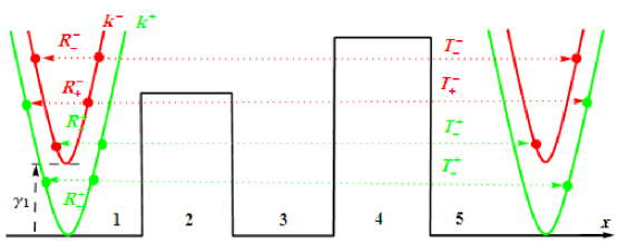
Figure 3: Schematic representation of different modes as well as the corrresponding transmission and reflection probabilities.

Figure 4 presents two different cases. (a): asymmetric double barrier structure for $U_{2}<U_{4}$, $\delta_{2}=\delta_{4}$ and (b): another symmetric one for $U_{2}=U_{4}$, $\delta_{2}=\delta_{4}$. It is interesting to note that the Ben results [30] can be recovered from our results by considering the case (b) and requiring $b=c$ in our double barrier structure. We notice that different channels of transmission and reflection in Figure 3 can be mapped into all cases in Figure 4 since they are related to the band structure on the both sides of the barriers. However, the effect of the different structure of the two barriers should appear in the transmission and reflection probabilities.

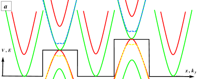
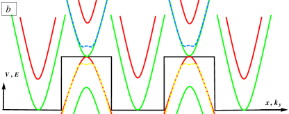
Figure 4: Scheme represents the bands inside and outside the barriers for the same interlayer potential difference. (a): asymmetric for $U_{2}<U_{4}$. (b): symmetric for $U_{2}=U_{4}$.

The solution of (10) can be written as a linear combination of plane waves

$$\phi_{B1}^{j}=a_{1}e^{ik^{+}_{j}x}+a_{2}e^{-ik^{+}_{j}x}+a_{3}e^{ik^{-}_{j}x}+a_{4}e^{-ik^{-}_{j}x}$$ (15)

where $a_{m}$ $(m=1,2,3,4)$ are coefficients of normalization. Substituting (15) into (6 -9) we obtain the rest of the spinor components:

$$\phi_{A1}^{j} = a_{1}A^{+}_{-}e^{ik^{+}_{j}x}-a_{2}A^{+}_{+}e^{-ik^{+}_{j}x}+a_{3}A^{-}_{-}e^{ik^{-}_{j}x}-a_{4}A^{-}_{+}e^{-ik^{-}_{j}x}$$ (16)

$$\phi_{A2}^{j} = a_{1}\rho^{+}e^{ik^{+}_{j}x}+a_{2}\rho^{+}e^{-jk^{+}_{j}x}+a_{3}\rho^{-}e^{ik^{-}_{j}x}+a_{4}\rho^{-}e^{-ik^{-}_{j}x}$$ (17)

$$\phi_{B2}^{j} = a_{1}\zeta^{+}_{+}e^{ik^{+}_{j}x}-a_{2}\zeta^{+}_{-}e^{-ik^{+}_{j}x}+a_{3}\zeta^{-}_{+}e^{ik^{-}_{j}x}-a_{4}\zeta^{-}_{-}e^{-ik^{-}_{j}x}$$ (18)

where we have set

$$A^{s}_{\pm}=\frac{l(k^{s}_{j}\pm ik_{y})}{\epsilon_{j}-\delta_{j}},\qquad\rho^{s}=(\epsilon_{j}-\delta_{j})\left[1-\frac{l^{2}\left[(k^{s}_{j})^{2}+k^{2}_{y}\right]}{(\varepsilon_{j}-\delta_{j})^{2}}\right],\qquad\zeta^{s}_{\pm}=\frac{\epsilon_{j}-\delta_{j}}{\epsilon_{j}+\delta_{j}}\rho^{s}A^{s}_{\pm}.$$ (19)

Now, we can write the general solution

$$\psi^{j}(x,y)=G_{j}M_{j}(x)C_{j}e^{ik_{y}y}$$ (20)

in terms of the matrices

$$G_{j}=\left(\begin{array}[]{cccc}A^{+}_{-}&-A^{+}_{+}&A^{-}_{-}&-A^{-}_{+}\\ 1&1&1&1\\ \rho^{+}&\rho^{+}&\rho^{-}&\rho^{-}\\ \zeta^{+}_{+}&-\zeta^{+}_{-}&\zeta^{-}_{+}&-\zeta^{-}_{-}\\ \end{array}\right),M_{j}=\left(\begin{array}[]{cccc}e^{ik^{+}_{j}x}&0&0&0\\ 0&e^{-ik^{+}_{j}x}&0&0\\ 0&0&e^{ik^{-}_{j}x}&0\\ 0&0&0&e^{-ik^{-}_{j}x}\\ \end{array}\right),C_{j}=\left(\begin{array}[]{c}a_{1}\\ a_{2}\\ a_{3}\\ a_{4}\\ \end{array}\right)$$ (21)

Since we are using the transfer matrix, we are interested in the normalization coefficients, the components of $C$, on the both sides of the double barrier. In other words, we need to specify our spinor in region 1

$$\phi^{1}_{A1} = \delta_{s,1}A^{+}_{-}e^{ik^{+}_{0}x}-r^{s}_{+}A^{+}_{+}e^{-ik^{+}_{0}x}+\delta_{s,-1}A^{-}_{-}e^{ik^{-}_{0}x}-r^{s}_{-}A^{-}_{+}e^{-ik^{-}_{0}x}$$ (22)

$$\phi^{1}_{B1} = \delta_{s,1}e^{ik^{+}_{0}x}+r^{s}_{+}e^{-ik^{+}_{0}x}+\delta_{s,-1}e^{ik^{-}_{0}x}+r^{s}_{-}e^{-ik^{-}_{0}x}$$ (23)

$$\phi^{1}_{A2} = \delta_{s,1}\rho^{+}e^{ik^{+}_{1}x}+r^{s}_{+}\rho^{+}e^{-ik^{+}_{0}x}+\delta_{s,-1}\rho^{-}e^{ik^{-}_{0}x}+r^{s}_{-}\rho^{-}e^{-ik^{-}_{0}x}$$ (24)

$$\phi^{1}_{B2} = \delta_{s,1}\zeta^{+}_{+}e^{ik^{+}_{0}x}-r^{s}_{+}\zeta^{+}_{-}e^{-ik^{+}_{0}x}+\delta_{s,-1}\zeta^{-}_{+}e^{ik^{-}_{0}x}-r^{s}_{-}\zeta^{-}_{-}e^{-ik^{-}_{0}x}$$ (25)

as well as region 5

$$\phi^{5}_{A1} = t^{s}_{+}A^{+}_{-}e^{ik^{+}_{0}x}+t^{s}_{-}A^{-}_{-}e^{ik^{-}_{0}x}$$ (26)

$$\phi^{5}_{B1} = t^{s}_{+}e^{ik^{+}_{0}x}+t^{s}_{-}e^{ik^{-}_{0}x}$$ (27)

$$\phi^{5}_{A2} = t^{s}_{+}\rho^{+}e^{ik^{+}_{0}x}+t^{s}_{-}\rho^{-}e^{ik^{-}_{0}x}$$ (28)

$$\phi^{5}_{B2} = t^{s}_{+}\zeta^{+}_{+}e^{ik^{+}_{0}x}+t^{s}_{-}\zeta^{-}_{+}e^{ik^{-}_{0}x}$$ (29)

Since the potential is zero in regions 1, 3 and 5, we have the relation

$$G_{1}M_{1}(x)=G_{3}M_{3}(x)=G_{5}M_{5}(x).$$ (30)

We will see how the above results will be used to determine different physical quantities. Specifically we focus on the reflection and transmission probabilities as well as related matters.

3 Transmission probabilities and conductance

Implementing the appropriate boundary condition in the context of the transfer matrix approach, one can obtain the transmission and reflection probabilities. Continuity of the spinors at the boundaries gives the components of the vector $C$ which are given by

$$C^{s}_{1}=\left(\begin{array}[]{cccc}\delta_{s,1}\\ r^{s}_{+}\\ \delta_{s,-1}\\ r^{s}_{-}\\ \end{array}\right),\qquad C^{s}_{5}=\left(\begin{array}[]{c}t^{s}_{+}\\ 0\\ t^{s}_{-}\\ 0\\ \end{array}\right)$$ (31)

where $\delta_{s,\pm 1}$ is the Kronecker delta symbol. The coefficients in the incident and reflected regions can be linked through the transfer matrix $M$

$$C^{s}_{1}=MC^{s}_{5}$$ (32)

which can be obtained explicitly by applying the continuity at the four boundaries of the double barrier structure (Figure 1). These are given by

$$G_{1}M_{1}(a)C_{1} = G_{2}M_{2}(a)C_{2}$$ (33)

$$G_{2}M_{2}(b)C_{2} = G_{3}M_{3}(b)C_{3}$$ (34)

$$G_{3}M_{3}(c)C_{3} = G_{4}M_{4}(c)C_{4}$$ (35)

$$G_{4}M_{4}(d)C_{4} = G_{5}M_{5}(d)C_{5}$$ (36)

Now solving the above system of equations and taking into account of the relation (30), one can find the form of $M$.

Then we can specify the complex coefficients of the transmission $t^{s}_{\pm}$ and reflection $r^{s}_{\pm}$ using the transfer matrix $M$. Since we need the transmission $T$ and reflection $R$ probabilities and because the velocity of the waves scattered through the two different modes is not the same, it is convenient to use the current density $\mathbf{J}$ to obtain the transmission and reflection probabilities.

$$\mathbf{J}=\nu_{F}{\mathbf{\Psi}}^{\dagger}\vec{\alpha}{\mathbf{\Psi}}$$ (37)

to end up with

$$T=\frac{|\mathbf{J}_{\sf tra}|}{|\mathbf{J}_{\sf inc}|},\qquad R=\frac{|\mathbf{J}_{\sf ref}|}{|\mathbf{J}_{\sf inc}|}$$ (38)

where $\vec{\alpha}$ is a $4\times 4$ diagonal matrix, on the diagonal 2 Pauli matrices $\sigma_{x}$. From (31) and (38), we show that the eight transmission and reflection probabilities are given by [32]

$$T^{s}_{\pm}=\frac{k^{\pm}_{0}}{k^{s}_{0}}|t^{s}_{\pm}|^{2},\qquad R^{s}_{\pm}=\frac{k^{\pm}_{0}}{k^{s}_{0}}|r^{s}_{\pm}|^{2}$$ (39)

These expressions can be explained as follows. Since we have four band, the electrons can be scattered between them and then we need to take into account the change in their velocities. With that, we find four channels in transmission and reflection such that $k_{0}^{\pm}$ is also given by (12). More precisely, at low energies $(E<\gamma_{1})$, we have just one mode of propagation $k_{0}^{+}$ leading to one transmission $T$ and reflection $R$ channel through the two conduction bands touching at zero energy on the both sides of the double barrier. Whereas at higher energy $(E>\gamma_{1})$, we have two modes of propagation $k_{0}^{+}$ and $k_{0}^{-}$ leading to four transmission $T^{\pm}_{\pm}$ and reflection $R^{\pm}_{\pm}$ channels, through the four conduction bands.

Since we have found transmission probabilities, let see how these will effect the conductance of our system. This actually can be obtained through the Landauer-Büttiker formula [31] by summing on all channels to end up with

$$\mathbf{G}(E)=G_{0}\frac{L_{y}}{2\pi}\int_{-\infty}^{+\infty}dk_{y}\sum_{s,n=\pm}T^{s}_{n}(E,k_{y})$$ (40)

where $L_{y}$ is the width of the sample in the $y$-direction and $G_{0}=4\ \frac{e^{2}}{h}$, the factor $4$ is due to the valley and spin degeneracy in graphene.

The obtained results will be numerically analyzed to discuss the basic features of our system and also make link with other published results. Because of the nature of our system, we do our task by distinguishing two different cases in terms of the band tunneling.

4 Two band tunneling

Barbier [27] investigated the transmission and conductance for single and multiple electrostatic barriers with and without interlayer potential difference and for $E<\ \gamma_{1}$, however the geometry dependance of the transmission was not done. In this section, we briefly investigate the resonances resulting from the available states in the well between the two barriers and how they influence by the geometry of the system.

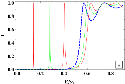
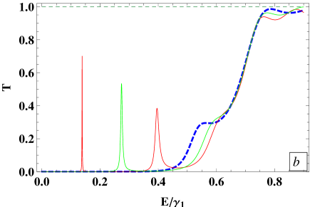
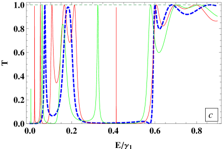
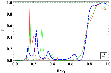
Figure 5: Transmission for normal incidence with $b_{1}=b_{2}=10\ nm$, and $\Delta=0$ (blue dashed), $\Delta=5\ nm$ (green), $\Delta=10\ nm$ (red). (a): $U_{2}=U_{4}=0.4\ \gamma_{1}$. (b): $U_{2}=0.4\ \gamma_{1}$ and $U_{4}=0.6\ \gamma_{1}$. (c,d): the same parameters as in (a,b), respectively, but with $\delta_{2}=\delta_{4}=0.2\ \gamma_{1}$.

For a normal incidence and for $\delta_{2}=\delta_{4}=0$ the transmission amplitude is shown in Figure 5a for different values of the distance $\Delta$ between the barriers. The dashed blue curve is for a single barrier with $(\Delta=0)$ and with width $(b_{1}+b_{2}=20\ nm)$, we note that the transmission is zero and there are no resonances in this regime of energy $(E<U_{2}=U_{4})$. Unlike the case of the single barrier, the double barrier structure has resonances in the above mentioned range of energy. These full transmission peaks can be attributed to the bound electron states in the well region between the barriers. In agreement with [33], the number of these resonances depends on the distance between the barriers. Indeed, for $\Delta=5\ nm$ we have one peak in the transmission amplitude, increasing the distance allows more bound states to emerge in the well, and for $\Delta=10\ nm$ there are two peaks (green and red curves in Figure 5, respectively). Figure 5b shows the same results in 5a but with different height of the two barriers such that $U_{2}=0.4\ \gamma_{1}$ and $U_{4}=0.6\ \gamma_{1}$. We see that the asymmetric structure of the double barrier reduces those resonances resulting from the bound electrons in the well between the two barriers. For $\delta_{2}=\delta_{4}=0.2\ \gamma_{1}$, we show the transmission probability by choosing $U_{2}=U_{4}=0.4\ \gamma_{1}$ in Figure 5c and for $U_{2}=0.4\ \gamma_{1}$, $U_{4}=0.6\ \gamma_{1}$ in Figure 5d. For single barrier, there are no resonant peaks inside the induced gap which is not the case for the double barrier as clarified in Figure 5c.

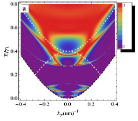
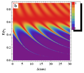
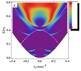
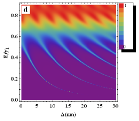
Figure 6: Density plot of transmission probability, for $\delta_{2}=\delta_{4}=0$, versus (a): $E$ and $ky$ for $U_{2}=U_{4}=0.4\ \gamma_{1}$, and $b_{1}=b_{2}=\Delta=10\ nm$, (b): $E$ and $\Delta$ with $ky=0$ and $b_{1}=b_{2}=10\ nm$, (c): $E$ and $ky$ with $U_{2}=0.4\ \gamma_{1}$, $U_{4}=0.6\ \gamma_{1}$ and $b_{1}=b_{2}=\Delta=10\ nm$, (d): $E$ and $\Delta$ with $U_{2}=0.4\ \gamma_{1}$, $U_{4}=0.6\ \gamma_{1}$, $ky=0$ and $b_{1}=b_{2}=10\ nm$. White and black dashed lines represent the band inside and outside the first barrier, respectively.

Figures 6a,6c present a comparison of the density plot of the transmission probability as a function of the transverse wave vector $k_{y}$ of the incident wave and its energy $E$ between different structure of the double barrier with $U_{2}=U_{4}=0.4\ \gamma_{1}$ and $U_{2}=0.4\ \gamma_{1}<U_{4}=0.6\ \gamma_{1}$, respectively, and for $\delta_{2}=\delta_{4}=0$ in both. For non-normal incidence in Figure 6a ($k_{y}\neq 0$) we still have a full transmission, even for energies less than the height of the barriers, which are symmetric in $k_{y}$. Those resonances are reduced and even disappeared in Figure 6c due to the asymmetric structurer of the double barrier. In Figures 6b,6d we show the density plot of transmission probability, for normal incidence, as a function of $\Delta$ and $E$ for the same parameters as in Figure 6a and 6c, respectively. We note that the number of resonances in Figure 6b, due to the bounded electrons in the well between the barriers, increases as long as the distance is increasing. They are very sharp for the low energies and become wider at higher energies. In contrast to Figure 6d and as a result of the asymmetric structure of the double barrier these resonances do not exist anymore for $E<U_{4}=0.6\ \gamma_{1}$.

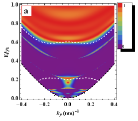
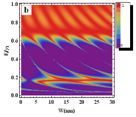
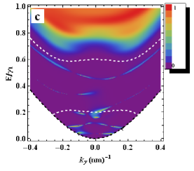
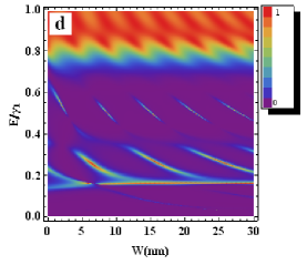
Figure 7: Density plot of transmission probability, for $\delta_{2}=\delta_{4}=0.2\ \gamma_{1}$, versus (a): $E$ and $k_{y}$ for $U_{2}=U_{4}=0.4\ \gamma_{1}$, and $b_{1}=b_{2}=\Delta=10\ nm$, (b): $E$ and $\Delta$ for the same parameters as in (a) but with $k_{y}=0$, (c,d): for the same parameters as in (a, b), respectively, but for $U_{2}=0.4\ \gamma_{1}$, $U_{4}=0.6\ \gamma_{1}$. White and black dashed lines represent the band inside and outside the first barrier, respectively.

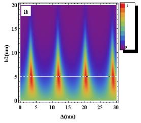
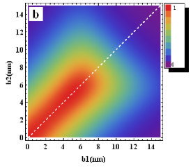
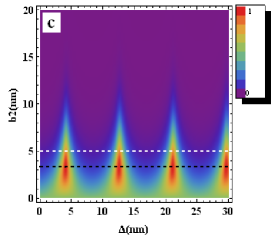
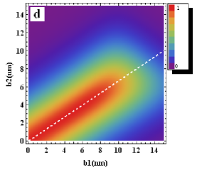
Figure 8: Density plot of transmission at normal incidence for $E=\frac{4}{5}\ U_{2}$ and $\delta_{2}=\delta_{4}=0$. (a): $U_{2}=U_{4}=0.4\ \gamma_{1}$, $b_{1}=5\ nm$. (b): $U_{2}=U_{4}=0.4\ \gamma_{1}$, $\Delta=3.36\ nm$. (c) $U_{2}=0.4\ \gamma_{1},U_{4}=0.6\ \gamma_{1}$, $b_{1}=5\ nm$. (d): $U_{2}=0.4\ \gamma_{1},U_{4}=0.6\ \gamma_{1}$, $\Delta=4\ nm$. The dashed white and black lines in the left column represent the values of $b_{1}$ and $b_{2}$, respectively, where the resonance occur.

It is well-known that introducing an interlayer potential difference induces an energy gap in the energy spectrum in bilayer graphene. It is worth to see how this interlayer potential difference will affect the transmission probability. To do so, we extend the results presented in Figure 6 to the case $\delta_{2}=\delta_{4}=0.2\ \gamma_{1}$ to get Figure 7. In agreement with [27], Figure 7a shows a full transmission inside the gap in the energy spectrum, which resulting from the available states in the well between the barriers. In contrast to the single barrier case [27, 30], there are full transmission inside the energy gap. In Figure 7b, we show the density plot of the transmission probability as a function of $E$ and $\Delta$ for fixed thickness of the tow barriers. We note that the resonances resulting from the bound states in the well are highly influenced by the interlayer potential difference where it removes part of them and arises a full transmission at specific value of the energy $E\approx 0.17\ \gamma_{1}$, which is absent in the case when there is no interlayer potential difference ($\delta_{2}=\delta_{4}=0$ in Figure 6b). Figures 7c,7d show the same result as in Figures 7a,7b, respectively, but with different heights of the barriers $U_{2}=0.4\ \gamma_{1}$ and $U_{4}=0.6\ \gamma_{1}$, which shows a decreasing in the transmission probability as a results of the asymmetric structure of the two barriers.

In Figure 8 we observe how these resonances for normal incidence are affected by the parameters of the barriers. In the first row we fixed the thickness of the first barrier $b_{1}=5\ nm$ and set the height of the two barriers to be the same $(U_{2}=U_{4}=0.4\ \gamma_{1})$, then we plot the transmission as a function of $\Delta$ and the thickness of the second barrier $b_{2}$ as depicted in Figure 8a. These resonances occur frequently as $\Delta$ increases where $b_{2}$ (dashed black line) is equal to $b_{1}$ (dashed wight line). Picking up one of these resonances (i.e. at fixed distance between barriers $\Delta=3.36\ nm$) and calculating the transmission as a function of $b_{1}$ and $b_{2}$ as presented in Figure 8b, it becomes clear that these resonances occur when $(b_{1}=b_{2})$ for fixed $\Delta$. In the second row, we show the transmission for the same parameters as in the first row but with different heights of the barriers $(U_{2}=0.4\ \gamma_{1},U_{4}=0.6\ \gamma_{1})$. Full transmission now occur for $b_{1}$ (dashed black line) $\neq b_{2}$ (dashed black line) as shown in Figure 8c. It is worth mentioning that for energies less than the strength of the barriers, and for a fixed $\Delta$, full transmission resonances occur always when $S_{1}=S_{2}$, $S_{1}$ and $S_{2}$ being the area of the first and second barrier, respectively. Therefore, for fixed $b_{1}$, the value of $b_{2}$ where the resonance occur is given by $b_{2}=\frac{U_{2}}{U_{4}}\ b_{1}$ which is superimposed in Figure 8b,8d (the dashed white line). Moreover, the cloak effect in the double barrier occur at non-normal incidence for some states which is different from the single barrier case [34] that occur always at normal incidence.

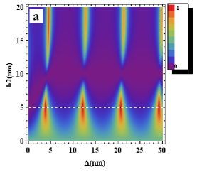
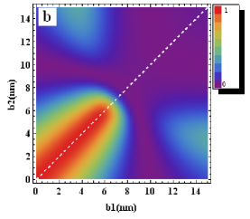
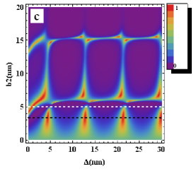
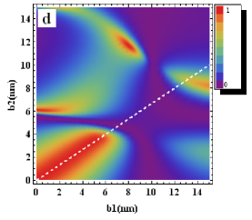
Figure 9: Density plot of transmission at normal incidence for $E=\frac{4}{5}\ U_{2}$ and $\delta_{2}=\delta_{4}=0.1\ \gamma_{1}$. (a): $U_{2}=U_{4}=0.4\ \gamma_{1}$, $b_{1}=5\ nm$. (b): $U_{2}=U_{4}=0.4\ \gamma_{1}$, $\Delta=3.7\ nm$. (c): $U_{2}=0.4\ \gamma_{1},U_{4}=0.6\ \gamma_{1}$, $b_{1}=5\ nm$. (d) $U_{2}=0.4\ \gamma_{1},U_{4}=0.6\ \gamma_{1}$, $\Delta=4.3\ nm$. The dashed white and black lines in the left column represent the values of $b_{1}$ and $b_{2}$, respectively, where the resonance occur.

In Figure 9 we extend the results in Figure 8 but with interlayer potential difference ($\delta_{2}=\delta_{4}=0.1\ \gamma_{1}$) for the same other parameters. As we note the total transmission probability is decreasing and some of the original resonances are splitting as a sequence of the induced energy gap. Let us now see how the transmission probability is affected by the double barrier parameters.

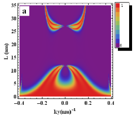
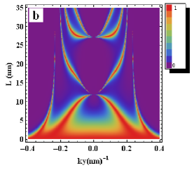
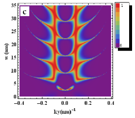
Figure 10: Density plot of the transmission probability versus (a,b): $k_{y}$ and the width of the two barriers $(b_{1}=b_{2}=L)$ for $U_{2}=U_{4}=0.6\ \gamma_{1}$, $E=\frac{4}{5}\ U_{4}$ and $\Delta=10\ nm,15\ nm$, respectively. (c): $k_{y}$ and $\Delta$ for the same parameters as in (a) and for $b_{1}=b_{2}=10\ nm$. (d): $ky$ and $b_{2}$ with $b_{1}=5\ nm$ and $\Delta=10\ nm$.

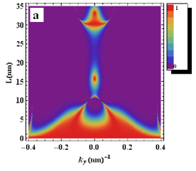
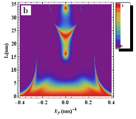
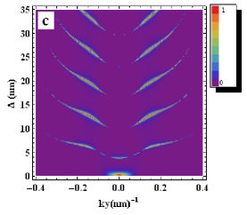
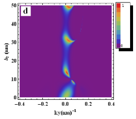
Figure 11: Density plot of the transmission probability versus (a,b): $k_{y}$ and the width of the two barriers $(b_{1}=b_{2}=L)$ for $U_{2}=U_{4}=0.6\ \gamma_{1}$, $E=\frac{4}{5}\ U_{4}$, $\delta_{2}=\delta_{4}=0.1\ \gamma_{1}$ and $\Delta=10\ nm,15\ nm$, respectively. (c): $k_{y}$ and the width of the well $\Delta$ for the same parameters as in (a) and for $b_{1}=b_{2}=10\ nm$. (d): $ky$ and $b_{2}$ with $b_{1}=5\ nm$ and $\Delta=10\ nm$.

In Figures 10a,10b we show the density plot of the transmission probability for $U_{2}=U_{4}$, $E<U_{2}=U_{4}$ and different values of $\Delta$, as a function of $k_{y}$ and the thickness of the two barriers $L$ (i.e. with changing the width of the two barriers simultaneously by setting $b_{1}=b_{2}=L$). For $\Delta=10\ nm$ and for small $L$ we have a full transmission for wide range of $k_{y}$, with increasing $L$, transmission probability dramatically decreases however, some resonances still show up as depicted in Figure 10a. In contrast, for $\Delta=15\ nm$ the transmission probability is completely different where the position and number of resonant peaks change as depicted in Figure 10b. This stress that the crucial parameters that determine the number of resonant peaks and their position is the width of the well $\Delta$ not the thickness of the two barriers $b_{1}$ and $b_{2}$[27, 33]. $\Delta$ dependance of the transmission probability is shown in Figure 10c, we note a full transmission frequently occur for normal incidence. Moreover, after certain value of $\Delta$ we start getting a full transmission for specific value of $k_{y}$ and for all values of $\Delta$. In Figure 10d we show how the transmission probability changes with $b_{2}$ and $k_{y}$ for fixed $\Delta$ and $b_{1}$.

The effect of the interlayer potential difference on the transmission probability with respect to the geometry of the barriers is depicted in Figure 11 for the same parameters as in Figure 10 but for $\delta_{2}=\delta_{4}=0.1\ \gamma_{1}$, we note that most of the resonances disappeared as one can conclude from Figure 10 due to the gap in the spectrum resulting from the induced electric field.

5 Four band tunneling

For energies larger than $\gamma_{1}$, the particles can use the two conduction band for propagation which gives rise to four channels of transmission and four for reflection. In Figure 12 we present these reflection and transmission probabilities for a double barrier structure as a function of $k_{y}$ and $E$. The potential barriers heights are set to be $U_{2}=U_{4}=\frac{3}{2}\ \gamma_{1}$ and the interlayer potential difference is zero. Different regions are shown up in the spectrum ($E,k_{y}$) which appeared as a result of the different propagating modes inside and outside the barriers. The superimposed dashed curves in the density plot in Figure 12 indicates the borders between these different regions [30]. In the double barrier, the cloak effect [34] in $T^{+}_{+}$ and $T^{+}_{-}$ $(T^{-}_{+})$ occurs in the region $U_{2}-\gamma_{1}<E<U_{2}$ for nearly normal incidence $k_{y}\approx 0$ where the two modes $k^{+}$ and $k^{-}$ are decoupled and therefore no scattering occurs between them [30]. However, this effect also exist for some states for non-normal incidence as a result of the available electrons states in the well as mentioned in the previous section. For non-normal incidence the two modes $k^{+}$ and $k^{-}$ are coupled and hence the electrons can be scattered between them, so that the transmission $T^{+}_{+}$ and $T^{+}_{-}$ $(T^{-}_{+})$ in the same region are not zero for non-normal incidence. For energies less than $U_{2}-\gamma_{1}$ electrons propagate via $k^{+}$ mode inside the barriers which give the resonances in $T^{+}_{+}$ in this region. Increasing (decreasing) the area of the barriers or the well between them will increase (decrease) the number of these resonances.

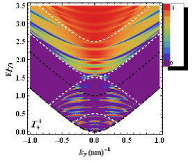
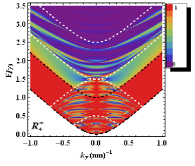
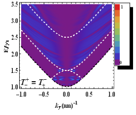
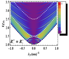
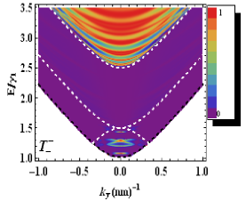
Figure 12: Density plot of transmission and reflection probabilities with $U_{2}=U_{4}=1.5\ \gamma_{1}$, $b_{1}=b_{2}=20\ nm$ and $\Delta=10\ nm$. The dashed white and black lines represent the band inside and outside the barrier, respectively.

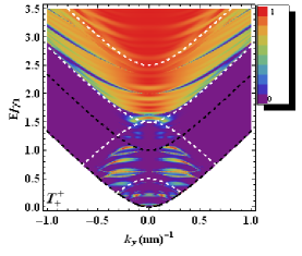
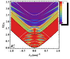
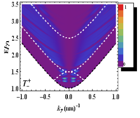
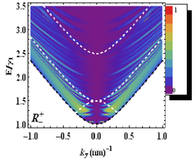
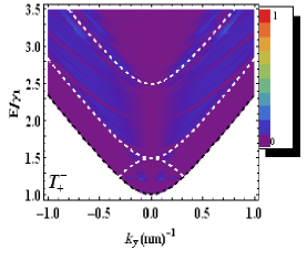
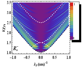
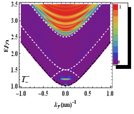
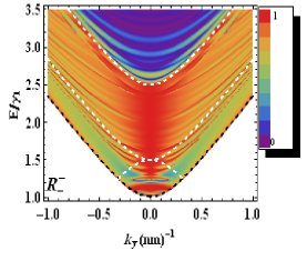
Figure 13: Density plot of transmission and reflection probabilities with $U_{2}=1.3\ \gamma_{1}$, $U_{4}=1.5\ \gamma_{1}$, $b_{1}=b_{2}=20\ nm$ and $\Delta=10\ nm$. The dashed white and black lines represent the band inside and outside the second barrier, respectively.

For $T^{-}_{-}$ electrons propagate via $k^{-}$ mode which is absent inside the barriers so that the transmission is suppressed in this region and this is equivalent to the cloak effect [30]. The transmission probabilities $T^{+}_{-}$ and $T^{-}_{+}$ are the same just when the time reversal symmetry holds (in this case when $\delta_{j}=0,\ U_{2}=U_{4}$) which means that electrons moving in opposite direction (moving from left to right and scattering from $k^{+}\rightarrow k^{-}$ in the vicinity of the first valley or moving from right to left and scattering from $k^{-}\rightarrow k^{+}$ in the vicinity of the second valley) are the same because of the valley equivalence [30].

Introducing asymmetric double barrier structure with $U_{2}=1.3\ \gamma_{1}$, $U_{4}=1.5\ \gamma_{1}$ and without interlayer potential difference will break this equivalence symmetry such that $T^{+}_{-}\neq T^{-}_{+}$ as depicted in Figure 13. In contrast, the reflection probabilities $R^{+}_{-}$ and $R^{-}_{+}$ stay the same because the incident electrons return again in an electron states [30]. In addition, the resonant peaks in $T^{+}_{+}$ are less intens comparing to $T^{+}_{+}$ with $U_{2}=U_{4}$ in Figure 12.

Now let see how the interlayer potential difference will affect the different channels of transmission and reflection. Figure 14 reveals the probabilities of the different transmission and reflection channels as a function of $k_{y}$ and $E$ for $U_{2}=U_{4}=1.5\ \gamma_{1}$ and $\delta_{2}=\delta_{4}=0.2\ \gamma_{1}$. The general behavior of these different channels resemble the single barrier case [30] with some major differences, such as observing extra resonances in the energy region $0<E<U_{j}$ due to these bounded states in the well. In addition, the induced gap does not completely suppressed the transmission in the energy region $U_{j}\pm\delta_{j}$ as it the case in the single barrier [30] and this is also attributed to these bounded states.

With the interlayer potential difference and different height of the barriers for $U_{2}=1.3\ \gamma_{1}$, $U_{4}=1.5\ \gamma_{1}$ and $\delta_{2}=\delta_{4}=0.2\ \gamma_{1}$ we show the different channels of transmission and reflection probabilities in Figure 15. In the same manner, the effect of this different height of the barriers is reducing the transmission probabilities. However, we note that it becomes more intens inside the gap and this is because the available states outside the first barrier which are in the same energy zone of the gap on the second barrier.

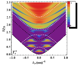
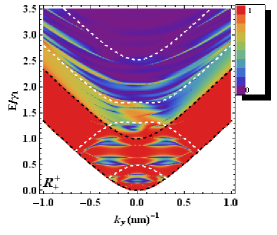
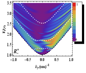
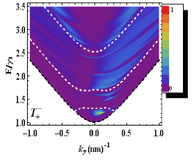
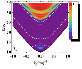
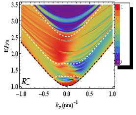
Figure 14: Density plot of transmission and reflection probabilities with $U_{2}=U_{4}=1.5\ \gamma_{1}$, $\delta_{2}=\delta_{4}=0.2\ \gamma_{1}$ and $b_{1}=b_{2}=\Delta=10\ nm$. The dashed white and black lines represent the band inside and outside the second barrier, respectively.

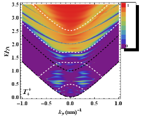
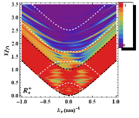
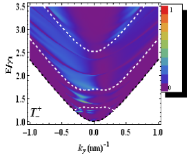
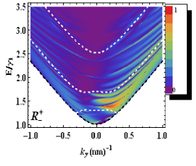
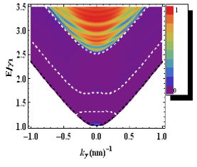
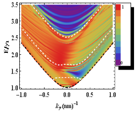
Figure 15: Density plot of transmission and reflection probabilities with $U_{2}=1.3\ \gamma_{1}$, $U_{4}=1.5\ \gamma_{1}$, $\delta_{2}=\delta_{4}=0.2\ \gamma_{1}$ and $b_{1}=b_{2}=\Delta=10\ nm$. The dashed white and black lines represent the band inside and outside the second barrier, respectively.

6 Conductance

In Figure 16 we show the conductance as a function of the energy $E$. Figure 16a shows the conductance of the double barrier structure for $U_{2}=U_{4}=1.5\ \gamma_{1}$, $\delta_{2}=\delta_{4}=0$ for $\Delta=5\ nm$ (dotted curve) and $\Delta=10\ nm$ (solid curve). The peaks in the conductance of the double barrier have extra shoulders as a results of the resonances in the transmission probabilities due to the existence of the bound electron states in the well. These resonances show up as convex curves, which were absent for the single barrier, in $T^{+}_{+}$ in the region $0<E<U_{2}=U_{4}$ and in $T^{+}_{-},T^{-}_{+}$ and $T^{-}_{-}$ in the region $\gamma_{1}<E<U_{2}=U_{4}$ as depicted in figure 12.

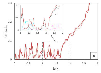
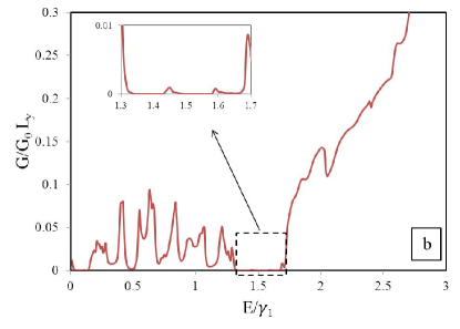
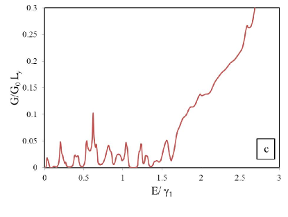
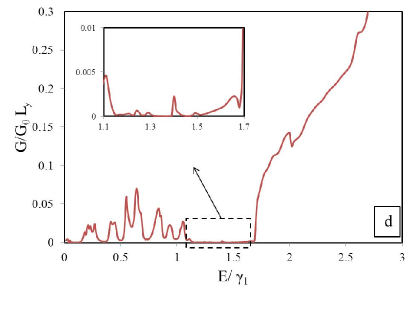
Figure 16: Conductance of the double barrier structure as a function of energy for $b_{1}=b_{2}=20\ nm$. (a) $U_{2}=U_{4}=1.5\ \gamma_{1}$, $\Delta=10\ nm$ (solid), $\Delta=5\ nm$ (dotted) and $\delta_{2}=\delta_{4}=0$. (b) $U_{2}=U_{4}=1.5\ \gamma_{1}$ and $\delta_{2}=\delta_{4}=0.2\ \gamma_{1}$. (c) $U_{2}=1.3\ \gamma_{1}$ , $U_{4}=1.5\ \gamma_{1}$, $\Delta=10\ nm$ and $\delta_{2}=\delta_{4}=0$. (d) $U_{2}=1.3\ \gamma_{1}$, $U_{4}=1.5\ \gamma_{1}$, $\Delta=10\ nm$ and $\delta_{2}=\delta_{4}=0.2\ \gamma_{1}$.

For energies larger than $U_{2}+\gamma_{1}$ the channel $T^{-}_{-}$ is not suppressed (cloaked) anymore so that we notice these very pronounced peaks in the conductance in this regime. The inset of Figure 16a show the contribution of each channel to the conductance for $\Delta=10\ nm$ in the region $\gamma_{1}<E<2\gamma_{1}$. For energies between the interlayer coupling and the barriers’s height all channel contribute to the conductance, but for energies larger than the barrier’s height the contribution of $T^{-}_{-}$ is zero due to the cloak effect which is clarified in the inset of Figure 16a. In Figure 16b we show the conductance of the double barrier with the interlayer potential difference $\delta_{2}=\delta_{4}=0.2\ \gamma_{1}$ and for the same height of the two barriers $U_{2}=U_{4}=1.5\ \gamma_{1}$. As a result of the none zero transmission inside the gap (see Figure 14) we also have none zero conductance inside the gap as clarified in the inset of Figure 16b. In Figure 16c we represent the result in Figure 16a but with asymmetric double barrier structure such that $U_{2}=1.3\ \gamma_{1}$ and $U_{4}=1.5\ \gamma_{1}$ for $\delta_{2}=\delta_{4}=0$, we see that the asymmetric structure of the double barrier reduces the conductance and even removing some shoulders of the peaks. The effect of the asymmetric double barrier structure together with the interlayer potential difference is presented in Figure 16d for $U_{2}=1.3\ \gamma_{1}$, $U_{4}=1.5\ \gamma_{1}$, $\delta_{2}=\delta_{4}=0.2\ \gamma_{1}$. Similarly to the previous case, the conductance here also decreases and some of the main peaks are removed as a consequence of this asymmetric structure of the double barriers and the induced gap in the spectrum. Although the interlayer potential difference is the same on the both barriers, the gap in the conductance is not anymore $2\ \delta_{2}=2\ \delta_{4}=0.4\ \gamma_{1}$ as the case in Figure 16c instead it becomes $3\ \delta_{2}=3\ \delta_{4}=0.6\ \gamma_{1}$ as depicted in the inset of Figure 16. Moreover, although at $E=U_{2}=U_{4}=V$ there are no available states, the conductance is not zero (in the single and double barrier) and this is due to the presence of resonant evanescent modes which are responsible for the pseudo-diffusive transport at the Dirac point [26].

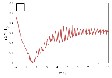
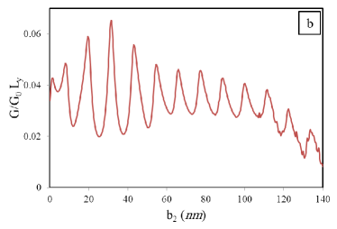
Figure 17: The conductance of the double barrier as a function of: (a) barriers’s height V ($U_{2}=U_{4}=$V) for $E=1.5\ \gamma_{1}$, $b_{1}=b_{2}=20\ nm$ and $\Delta=10\ nm$. (b) $b_{2}$ for V$=1.5\ \gamma_{1}$, $E=1.3\ \gamma_{1}$, $b_{1}=20\ nm$ and $\Delta=10\ nm$. (c) $\Delta$ for V$=1.5\ \gamma_{1}$, $E=1.3\ \gamma_{1}$ and $b_{1}=b_{2}=20\ nm$.

The conductance dependance on the double barriers parameters is shown in Figure 17. For $E=1.5\ \gamma_{1}$ and $\delta_{2}=\delta_{4}=0$ we show the conductance as a function of the height of the barriers V ($U_{2}=U_{4}=V$) in Figure 17a. In the region $E>$V$>0$ the conductance decreases with increasing $V$, whereas in the region $V>E$ it increases with increasing $V$ till it reaches a Plato constant value which is an odd behavior. This behavior is attributed to the resonance in the region $E<V$ since the conductance is minimum at the Dirac point (in this case $E=V$) leading to an increase of the conductance on the both sides of the Dirac point ( $E>V$ and $E<V$) [26]. In contrast, increasing $b_{2}$ for fixed other parameters decreases the conductance as depicted in Figure 17b and the number of resonances appearing in the conductance remains the same with increasing $b_{2}$. Finally, in Figure 17c we plot the conductance versus $\Delta$. The conductance is seen to oscillate with increasing width of the well and then reaches to a constant asymptotic value.

The transmissions coefficients of these evanescent modes are shown in Figure 18a,18b for a single and double barrier, respectively. At high potential strength $(\ U_{2}=U_{4}=V\gg\gamma_{1})$ and for $\delta_{2}=\delta_{4}=0$, the four channels at $E=V$ will give almost identical contributions, $T_{+}^{+}=T_{+}^{-}=T_{-}^{+}=T_{-}^{-}$, for single and double barrier because the electrons now can not differentiate between the two modes, see Figure 18c,18d.

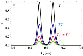
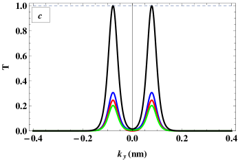
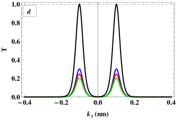
Figure 18: The transmissions coefficients around the Dirac point for $(E=V=1.5\ \gamma_{1})$ and $b_{1}=b_{2}=20\ nm$. (a) single barrier with $\Delta=0$. (b) double barrier with $\Delta=10\ nm$. (c, d) single and double barrier transmission for the same parameters as in (a, b), respectively, but for ($E=V=5\ \gamma_{1}$). Where $T=\sum_{s,n=\pm}(T^{s}_{n})$

7 Conclusion

In conclusion, we have evaluated the reflection and transmission probabilities of electrons through symmetric and asymmetric double barrier potential in a bilayer graphene system. Based on the four band model we found the solution in each potential region and by matching them at the interface of each region and obtained the different transmission and reflection coefficients. Subsequently, the transmission of electrons through symmetric and asymmetric double barrier structure for various barriers parameters was investigated for energy ranges $E<\gamma_{1}$ and $E>\gamma_{1}$ where there occurs one and two propagating mode, respectively.

We compared our results with previous work [34] (For $E<\gamma_{1}$) and showed that the cloak effect may occur for non-normal incidence and exhibits a sequence of the resonances in the transmission in the region $E<V$ due to bounded electrons in the well between the two barriers. Furthermore, for normal incidence we found that these resonances, which were absent for the single barrier, always occur for fixed energy ($E<U_{j}$) when $S_{1}=S_{2}$ where $S_{1},S_{2}$, that it requires equality of the areas of the first and second barrier. We also found that the most important parameter that control the position and the number of these resonances, in both cases $E<\gamma_{1}$ or $E>\gamma_{1}$, is the well width between the tow barriers not the thickness of the barriers in agreement with [27, 33].

Introducing the interlayer potential difference open a gap in the density plot of the transmission probabilities where it is not completely suppressed as it the case in the single barrier [30]. This is a consequence of the bound states in the well between the two barriers. The asymmetric structure of the double potential barrier reduces the transmission probabilities and removes the sharp resonant peaks. We observed that the resulting conductance for the double barrier was different from that of the single barrier. This difference manifests itself through the presence of many extra resonances which are associated with the bound electron states in the well.

The effect of the interlayer potential difference on the transmission probabilities is reflected on the conductance where we obtain a gap with non zero conductance. Moreover, the asymmetric structure of the double barrier reduces the conductance and removes the shoulders of main peaks. Finally, we studied the conductance dependance on the double barrier parameters. The conductance as a function of the height of the barrier showed a region where it increases with increasing the potential height, this is an odd behavior which can be correlated to the minimum conductance around the Dirac point.

References

- [1] A.K. Geim, and K.S. Novoselov, Nature Materials 6, 183 (2007).
- [2] H. Brody, Nature (London) 483, S29 (2012).
- [3] O. Klein, Zeitschrift für Physik 53, 157 (1929).
- [4] M.I. Katsnelson, K.S. Novoselov, and A.K. Geim, Nature Physics 2, 620 (2006).
- [5] S.Y. Zhou, D.A. Siegel, A.V. Fedorov, F. El Gabaly, A.K. Schmid, A.H. Castro Neto and A. Lanzara, Nature Materials 7, 259 (2007).
- [6] R. Costa Filho, G. Farias, and F. Peeters, Physical Review B 76, 193409 (2007).
- [7] Y. Zhang, T.-T. Tang, C. Girit, Z. Hao, M.C. Martin, A. Zettl, M.F. Crommie, Y.R. Shen, and F. Wang, Nature 459, 820 (2009).
- [8] E. McCann, Physical Review B 74, 1 (2006).
- [9] J.D. Bernal, Proceedings of the Royal Society A: Mathematical, Physical and Engineering Sciences 106, 749 (1924).
- [10] C. Bena, and G. Montambaux, New Journal of Physics 11, 095003 (2009).
- [11] S.B. Trickey, F. M ller-Plathe, and G.H.F. Diercksen, Physical Review B 45, 4460 (1992).
- [12] E. McCann, and V. Fal’ko, Physical Review Letters 96, 1 (2006).
- [13] E. McCann, D.S.L. Abergel, and V.I. Fal ko, Solid State Communications 143, 110 (2007).
- [14] E. McCann, D.S.L. Abergel, and V.I. Fal’ko, The European Physical Journal Special Topics 148, 91 (2007).
- [15] Z. Li, E. Henriksen, Z. Jiang, Z. Hao, M. Martin, P. Kim, H. Stormer, and D. Basov, Physical Review Letters 102, 16 (2009).
- [16] M. Koshino, New Journal of Physics 11, 095010 (2009).
- [17] A.H. Castro Neto, F. Guinea, N.M.R. Peres, K.S. Novoselov, and A.K. Geim, Reviews of Modern Physics 81, 109 (2009).
- [18] M. Killi, S. Wu, and A. Paramekanti, Physical Review Letters 107, 2 (2011).
- [19] S. Das Sarma, S. Adam, E. Hwang, and E. Rossi, Reviews of Modern Physics 83, 407 (2011).
- [20] A. Lherbier, S.M.-M. Dubois, X. Declerck, Y.-M. Niquet, S. Roche, and J.-C. Charlier, Physical Review B 86, 075402 (2012).
- [21] E. McCann and M. Koshino, Reports on Progress in Physics. Physical Society (Great Britain) 76, 056503 (2013).
- [22] H. Bahlouli, E.B. Choubabi, and A. Jellal, Europhysics Letters 95, 17009 (2011).
- [23] H. Bahlouli, E.B. Choubabi, A. Jellal, and M. Mekkaoui, Journal of Low Temperature Physics 169, 51 (2012).
- [24] A. Jellal, E.B. Choubabi, H. Bahlouli, and A. Aljaafari, Journal of Low Temperature Physics 168, 40 (2012).
- [25] A. El Mouhafid and A. Jellal, Journal of Low Temperature Physics 173, 264 (2013).
- [26] I. Snyman and C. Beenakker, Physical Review B 75, 045322 (2007).
- [27] J.M. Pereira, P. Vasilopoulos, and F.M. Peeters, Physical Review B 79, 155402 (2009).
- [28] M. Barbier, P. Vasilopoulos, and F.M. Peeters, Physical Review B 82, 235408 (2010).
- [29] T. Tudorovskiy, K.J. A. Reijnders, and M.I. Katsnelson, Physica Scripta T146, 014010 (2012).
- [30] B. Van Duppen and F.M. Peeters, Physical Review B 87, 205427 (2013).
- [31] Ya. M. Blanter, and M. Büttiker, Physics Reports 336, (2000).
- [32] B. Van Duppen, S.H.R. Sena, and F.M. Peeters, Physical Review B 87, 195439 (2013).
- [33] C. Bai, and X. Zhang, Physical Review B 76, 075430 (2007).
- [34] N. Gu, M. Rudner, and L. Levitov, Physical Review Letters 107, 156603 (2011).