Shape, Thermal and Surface Properties determination of a Candidate Spacecraft Target Asteroid (175706) 1996 FG3

Abstract

In this paper, a 3D convex shape model of (175706) 1996 FG3, which consists of 2040 triangle facets and 1022 vertices, is derived from the known lightcurves. The best-fit orientation of the asteroid’s spin axis is determined to be $\lambda=237.7^{\circ}$ and $\beta=-83.8^{\circ}$ considering the observation uncertainties, and its rotation period is $\sim$ 3.5935 h . Using the derived shape model, we adopt the so-called advanced thermophysical model (ATPM) to fit three published sets of mid-infrared observations of 1996 FG3 (Wolters et al., 2011; Walsh et al., 2012), so as to evaluate its surface properties. Assuming the primary and the secondary bear identical shape, albedo, thermal inertia and surface roughness, the best-fit parameters are obtained from the observations. The geometric albedo and effective diameter of the asteroid are reckoned to be $p_{\rm v}=0.045\pm 0.002$, $D_{\rm eff}=1.69^{+0.05}_{-0.02}$ km. The diameters of the primary and secondary are determined to be $D_{1}=1.63^{+0.04}_{-0.03}$ km and $D_{2}=0.45^{+0.04}_{-0.03}$ km, respectively. The surface thermal inertia $\Gamma$ is derived to be a low value of $80\pm 40\rm~{}Jm^{-2}s^{-0.5}K^{-1}$ with a roughness fraction $f_{\rm R}$ of $0.8^{+0.2}_{-0.4}$. This indicates that the primary possibly has a regolith layer on its surface, which is likely to be covered by a mixture of dust, fragmentary rocky debris and sand. The minimum regolith depth is estimated to be $5\sim 20\rm~{}mm$ from the simulations of subsurface temperature distribution, indicating that 1996 FG3 could be a very suitable target for a sample return mission.

1 Introduction

(175706) 1996 FG3 (hereafter, 1996 FG3) is a binary near-Earth asteroid (NEA) belonging to the Apollo type, which has a very low $\Delta$v value $\sim$ $5.16\rm~{}kms^{-1}$ (Perozzi et al., 2001; Christou, 2003). This asteroid was originally chosen as the target for a proposed sample return mission (Barucci et al., 2012), called MarcoPolo-R.

Eclipse events have been observed in the binary system 1996 FG3 in optical wavelengths (Pravec et al., 2000; Mottola & Lahulla, 2000). The period of mutual orbit is $16.14\pm 0.01\rm~{}hr$, and the diameter ratio $D_{2}/D_{1}$ is $0.28^{+0.01}_{-0.02}$ (Scheirich & Pravec, 2009). The primary is assumed to be an oblate ellipsoid with a major axis ratio $a/b\sim 1.2$, while the secondary is prolate with a major axis ratio about 1.4. Furthermore, Scheirich & Pravec (2009) showed the rotation period of the primary is $\sim 3.6\rm~{}hr$, and the mass density $1.4^{+1.5}_{-0.6}$ g cm^-3, where 1996 FG3 is generally classified as a complex C-type (Binzel et al., 2001, 2012; de León et al., 2011, 2013; Rivkin et al., 2013). The optical magnitude and phase coefficient are derived as $H=17.76\pm 0.03$ and $G=-0.07\pm 0.02$ by Pravec et al. (2006), while Wolters et al. (2011) used additional data to derive $H=17.833\pm 0.024$ and $G=-0.041\pm 0.005$.

Mueller et al. (2011) obtained an area-equivalent diameter of $1.8^{+0.6}_{-0.5}\rm~{}km$ and a geometric albedo of $p_{v}=0.04^{+0.04}_{-0.02}$ for 1996 FG3, based on thermal observations (3.6 and $4.5\rm~{}\mu m$) from the ”Warm Spitzer” space telescope. Furthermore, Wolters et al. (2011) measured the effective diameter and geometric albedo of the asteroid to be $D_{\rm eff}=1.68\pm 0.25\rm~{}km$, $p_{v}=0.046\pm 0.014$, $\eta=1.15$ for a solar phase angle $11.7^{\circ}$ from an NEATM (Harris, 1998; Delbo & Harris, 2002) procedure. In addition, using NEATM method, Walsh et al. (2012) also obtained 1996 FG3’s effective diameter and geometric albedo of $D_{\rm eff}=1.90\pm 0.28\rm~{}km$, $p_{v}=0.039\pm 0.012$, beaming parameter $\eta=1.61\pm 0.08$, for a phase angle $67.4^{\circ}$.

Walsh et al. (2008) modeled the formation of the binaries to be a history of rotation acceleration due to the YORP mechanism. Generally, the asymmetric reflection of sunlight and asymmetric thermal emission from an asteroid’s surface produces a net force and a net torque. The net force causes the orbit of the asteroid to drift, i.e., Yarkovsky effect, and the net torque alters its rotation period and direction of its rotation axis, i.e., YORP effect (Rozitis & Green, 2012). The asymmetric shape of an asteroid, as well as the existence of its finite rotation period and thermal inertia, plays a major role in affecting Yarkovsky and YORP effects. Thermal inertia is an important parameter that controls temperature distribution over the surface and sub-surface of the asteroid, and it is defined by $\Gamma=\sqrt{\rho c\kappa}$, where $\rho$ is the mass density, $\kappa$ the thermal conductivity, and $c$ the specific heat capacity. According to the definition, thermal inertia depends mainly on the regolith particle size and depth, degree of compaction, and exposure of solid rocks and boulders within the top few centimeters of sub-surface (Rozitis & Green, 2011). Therefore, thermal inertia may act as a vital indicator to infer the presence or absence of loose material on the asteroid’s surface.

The thermal inertia of an asteroid may be evaluated by fitting mid-infrared observations by applying a thermal model to reproduce mid-IR emission curves. Lagerros (1996) proposed a so-called thermophysical model (TPM), which is adopted to calculate infrared emission fluxes as a function of the asteroid’s albedo, thermal inertia, correction factor and so on. For example, we provide several values of $\Gamma$ for the targets of complete/future asteroid missions. On the basis of TPM, M$\ddot{u}$ller et al. (2005) measured the thermal inertia of asteroid (25143) Itokawa to be $\sim$ $750\rm~{}Jm^{-2}s^{-0.5}K^{-1}$. Again, M$\ddot{u}$ller et al. (2011) showed that the $\Gamma$ of 1999 JU3 is likely to be in the range of $200\sim 600\rm~{}Jm^{-2}s^{-0.5}K^{-1}$. The average thermal inertia of 1999 RQ36 is estimated to be $\sim$ $650\rm~{}Jm^{-2}s^{-0.5}K^{-1}$ (M$\ddot{u}$ller et al., 2012). Recently, Rozitis & Green (2011) proposed an advanced thermophysical model (ATPM) to extensively investigate the thermal nature of the asteroid. Subsequently, Wolters et al. (2011) obtained a best-fit thermal inertia $\Gamma=120\pm 50\rm~{}Jm^{-2}s^{-0.5}K^{-1}$ for 1996 FG3 with ATPM.

The structure of the paper is as follows. Firstly, Section 2 gives a brief introduction to the thermophysical model developed by Rozitis & Green (2011). In Section 3, we concentrate our study on deriving a new 3D shape model for the primary of 1996 FG3 from the known optical lightcurves (Pravec et al., 2000; Mottola & Lahulla, 2000; Wolters et al., 2011). The rotation period and spin axis of the primary are again updated in this work but they appear to be slightly different from those of Scheirich & Pravec (2009). Subsequently, in Section 4, we independently develop computation codes that duplicates ATPM (Rozitis & Green, 2011), and then carry out extensive fittings using three sets of mid-infrared observations of 1996 FG3 (Wolters et al., 2011; Walsh et al., 2012) to investigate the primary’s surface physical properties, such as the average thermal inertia, geometric albedo and roughness. The results show that this asteroid may have a very rough surface, in the meanwhile the thermal inertia and geometric albedo seem to be relatively low, indicative of the existence of loose material or regolith spreading over the asteroid’s surface. Moreover, Section 5 deals with the global surface and sub-surface temperature distribution at the aphelion and perihelion, and the minimum depth of regolith layer over the very surface of the primary from the simulations. In final, Section 6 presents the primary results of this work and gives a concise discussion.

2 Theory Method

2.1 Advanced Thermophysical Model

An asteroid is assumed to be a polyhedron composed of N triangle facets in ATPM. For each facet, the conservation of energy leads to the surface boundary condition (Rozitis & Green, 2011)

$$(1-A_{B})(s_{i}\psi_{i}F_{Sun}+F_{scat})+(1-A_{th})F_{red}=$$

$$\varepsilon\sigma T^{4}\big{|}_{z=0}+(-\kappa\frac{dT}{dZ})\Big{|}_{z=0},$$ (1)

where $A_{B}$ is the Bond albedo, $s_{i}$ indicates whether facet $i$ is illuminated by the Sun, $\varepsilon$ is the thermal emissivity, $\sigma$ the Stefan-Boltzmann constant, $\kappa$ the thermal conductivity, and $z$ the depth below the surface, respectively. $\psi_{i}$ means a function that returns the cosine of the sunlight incident angle. $F_{Sun}$ is the integrated solar flux at the distance of the asteroid, which can be approximated by

$$F_{Sun}=\frac{F_{\odot}}{r_{\odot AU}^{2}},$$ (2)

where $F_{\odot}$ is the solar constant, about $1367.5Wm^{-2}$, and $r_{\odot AU}$ is the heliocentric distance in AU. $F_{scat}$ and $F_{red}$ are the total multiple-scattered and thermal-radiated fluxes incident onto the facet from other facets, respectively. $A_{th}$ is the albedo of the surface at thermal-infrared wavelengths.

Temperature $T$ can be written as a function of time $t$ and depth $z$, i.e., $T(t,z)$. It can be described by one-dimension (1D) heat diffusion equation

$$\rho c\frac{\partial T}{\partial t}=\kappa\frac{\partial^{2}T}{\partial z^{2}},$$ (3)

For the asteroid, which may have a regolith layer over its surface, the temperature below the surface regolith is supposed to be constant. Thus an internal boundary condition could be given by

$$\frac{\partial T}{\partial z}\Big{|}_{z\rightarrow\infty}\rightarrow 0~{}.$$ (4)

Theoretically, the temperature distribution can be directly obtained by solving equation (3) and the boundary conditions of equations (1) and (4). However, the surface boundary condition is a nonlinear equation, thus we will attempt to solve them with numerical methods.

In order to simplify the solution of this problem, it is useful to introduce a standard transformation (Spencer & Lebofsky, 1989; Lagerros, 1996) as follows:

$$x = \frac{z}{l_{s}},$$

$$\tau = \omega t,$$

$$u = \frac{T}{T_{e}},$$

where

$$l_{s}=\sqrt{\frac{\kappa}{\rho c\omega}}$$

is referred to as skin depth. And

$$T_{e}=\left(\frac{(1-A_{B})F_{Sun}}{\varepsilon\sigma}\right)^{1/4}~{},$$ (5)

is called effective temperature.

Thus, the 1D heat diffusion equation is rewritten as

$$\frac{\partial u}{\partial\tau}=\frac{\partial^{2}u}{\partial x^{2}},$$ (6)

while the surface boundary condition and internal boundary condition are converted into

$$u^{4}\big{|}_{x=0}-\Phi\frac{du}{dx}\Big{|}_{x=0}=p_{1}+p_{2}+p_{3},$$ (7)

$$\frac{\partial u}{\partial x}\Big{|}_{x\rightarrow\infty}\rightarrow 0$$ (8)

where

$$p_{1} = s\cdot\psi,$$

$$p_{2} = (1-A_{B})\frac{F_{scat}}{\varepsilon\sigma T^{4}_{e}},$$

$$p_{3} = (1-A_{th})\frac{F_{red}}{\varepsilon\sigma T^{4}_{e}},$$

and

$$\Phi=\frac{\Gamma\sqrt{\omega}}{\varepsilon\sigma T^{3}_{e}}$$ (9)

$\Gamma$ is the thermal inertia, and $\Phi$ is the thermal parameter.

By numerically solving equation (6) with boundary condition equations (7) and (8), we can acquire the global temperature distribution over the surface and sub-surface of the asteroid. According to the theory, the program codes are also developed for investigation. In the following, we will introduce the results based on numerical calculations.

2.2 Emission Flux

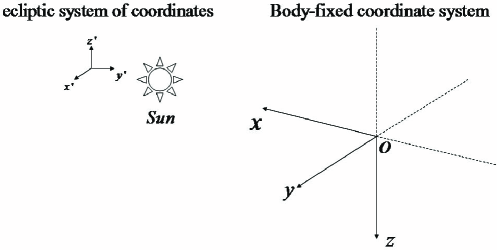
Figure 1: The coordinate system adopted in the model, where $O$ is the center of the asteroid, and z-axis is the spin axis.

On the basis of surface temperature distribution calculated from ATPM, we may estimate thermal infrared fluxes from the asteroid for a given phase angle $\alpha$ and geocentric distance $\Delta$. First of all, a body-fixed coordinate system is established (see Figure 1), where the origin $O$ locates at the center of asteroid, z-axis is parallel to its spin axis, and x-axis is chosen to remain in a plane determined by z-axis and the line of sun-asteroid, directing towards the Sun.

The direction vector of Earth in the body-fixed system is calculated from the asteroid’s orbit, expressed as $\vec{n}_{\oplus}$. Normal vector of each facet $\vec{n}_{i}$ is determined from the shape model of the asteroid. Hence, the view factor of each facet relative to Earth can be evaluated by

$$f(i)=v(i)A(i)\frac{\vec{n}_{i}\cdot\vec{n}_{\oplus}}{\pi\Delta^{2}}$$ (10)

where $v(i)=1$ indicates that facet $i$ can be seen from Earth, otherwise $v(i)=0$, and $A(i)$ is the area of facet $i$.

The flux emitted by each facet is described by the Plank function

$$B(\lambda,T_{i})=\frac{2\pi hc^{2}}{\lambda^{5}}\frac{1}{\exp\big{(}\frac{hc}{\lambda kT_{i}}-1\big{)}}$$ (11)

Consequently, the total fluxes observed from Earth are fully integrated over each facet

$$F_{\lambda}=\sum^{N}_{i=1}\varepsilon f(i)B(\lambda,T_{i})$$ (12)

3 Shape Model

According to direct images from space missions and radar measurements, the asteroids in small-size have an irregular shape, while those larger objects appear to be relatively regular shape. For instance, Vesta seems to be more circular than Eros. Considering the asteroid’s rotation, the observed lightcurves change with a lot of extrema, which provide key information on modeling its shape and morphology. Hence, the substantial shape and spin status of the asteroid can be derived from the observations. Kaasalainen & Torppa (2001) and Kaasalainen et al. (2001) developed the lightcurve inverse scheme, and in their model, the inverse problem is perfectly solved using modern deconvolution method and optimization techniques. With the assistance of the optical data, a convex shape of asteroid will be obtained. After repeating the fitting of the convex shape and additional observations, an improved shape of the asteroid will be better constructed. The relative chi-square is defined as

$$\chi^{2}_{rel}=\sum_{i}\|\frac{L^{(i)}_{obs}}{\bar{L}^{(i)}_{obs}}-\frac{L^{(i)}}{\bar{L}^{(i)}}\|^{2},$$ (13)

where $L^{(i)}$ and $L^{(i)}_{obs}$ are the modeled and observed brightness from lightcurves, respectively. $\bar{L}^{(i)}_{obs}$ and $\bar{L}^{(i)}$ are the averaged brightness of the observed data and the model, respectively. At the end of iteration, chi-square will approach a tiny value. Usually, for an asteroid, there are a great many of observations with respect to various solar angles at different epochs. Therefore, such method will yield a reliable result for the shape model.

Table 1: 14 lightcurves adopted in the shape model of 1996 FG3.

ID	Obs. Date	Obs. Number	References
1	1998-12-13	155	Mottola & Lahulla (2000)
2	1998-12-14	157	Mottola & Lahulla (2000)
3	1998-12-15	156	Mottola & Lahulla (2000)
4	1998-12-16	166	Mottola & Lahulla (2000)
5	1998-12-10	111	Pravec et al. (2000)
6	1998-12-17	110	Pravec et al. (2000)
7	1999-01-09	237	Pravec et al. (2000)
8	2009-03-25	16	(MPC)
9	2009-03-27	14	(MPC)
10	2009-03-28	21	(MPC)
11	2009-03-29	20	(MPC)
12	2009-04-22	17	(MPC)
13	2011-01-29	35	(Wolters et al., 2011)
14	2011-03-06	79	(Wolters et al., 2011)

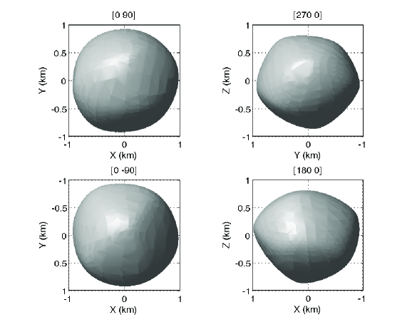
Figure 2: Derived shape model of 1996 FG3 shown from four view angles, i.e., north pole (top left), south pole (bottom left), equator (top right and bottom right), respectively.

As 1996 FG3 is a binary asteroid, the values of the brightness in the lightcurves consist of dual contributions coming from the primary and secondary. Similar characteristic of the lightcurves is shown by 1994 AW1 and 1991 VH (Pravec et al., 1997, 1998). Thus, it is clear that one cannot directly utilize the original data to construct the primary’s shape model. From the point of view of shape reconstruction, we should retrieve the short-period component from the observations in the very beginning. In the following, we describe the method that detaches the short-period and long-period components.

By taking outside the deep minima from the long-period component, the short-period component can be obtained. Then, applying the Fourier fitting of the lightcurves to only short-period component, the rotational profile for the primary can be detached (Mottola & Lahulla, 2000; Pravec et al., 2000). The Fourier series is in the form of (Harris, 1989; Pravec et al., 1996)

$$R(t)=C_{0}+\sum^{m}_{n=1}\left(C_{n}\cos\frac{2\pi n}{P}(t-t_{0})+S_{n}\sin\frac{2\pi n}{P}(t-t_{0})\right),$$ (14)

where $R$ is the magnitude computed at time $t$, the period $P=3.5942\pm 0.0002$ h, $t_{0}$ is the epoch, $C_{0}$, $C_{n}$ and $S_{n}$ are the mean magnitude and the Fourier coefficients of the $n$th order, respectively. Subtracting the short-period component from the observation data by assuming the long-period added to the short-period linearly in irradiance, two kinds of components can be gained.

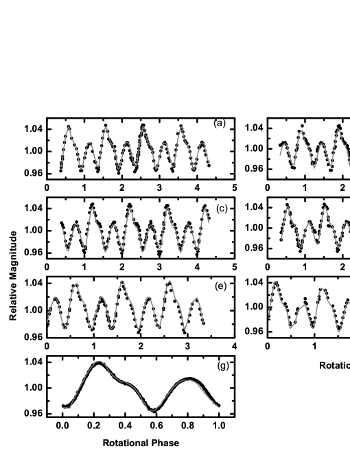
Figure 3: Comparison between the observed and modeling lightcurves. The red solid line means the modeling lightcurve while the black dot represents the observations. Panel (a) to (g) are the results of the cases with the first seven lightcurves (see Table 1).

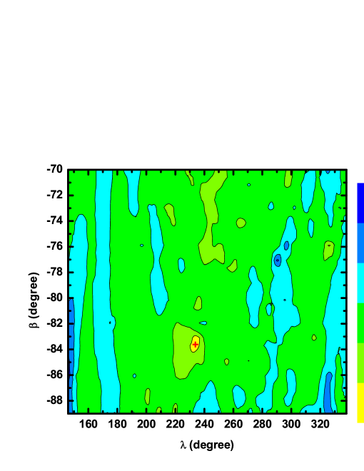
Figure 4: Contour of $\chi^{2}$ value. $\lambda$ and $\beta$ are chosen in their uncertainties of observed value. The red cross represents the pole orientation we determined from the shape model inversion process.

By subtracting short-period data, the long-period measurements show the information of eclipses/occultations which is not enough for the shape reconstruction of the secondary. Herein, we simply make use of the short-period data presented by the measurements that have been published already to precisely reconstruct the shape of the primary. We have already collected all optical data from 1996 to now, where there are 14 lightcurves of 1996 FG3 (see Table 1) in total (Mottola & Lahulla, 2000; Pravec et al., 2000, 2006; Scheirich & Pravec, 2009; Wolters et al., 2011). From the observation data of one to seven lightcurves, the best-fit fifth-order Fourier series separates the short-period component and the r.m.s residual is comparable to the observation errors. We can obtain the short-period data of the first seven lightcurves, where the first four lightcurves are adopted from Figure 1 of Mottola & Lahulla (2000), while the data of the fifth to seventh lightcurves are from Figures 1 to 3 of Pravec et al. (2000). The short-period component of the first seven lightcurves has already obtained in the published papers. In the observation interval of the remaining lightcurves, no eclipsed or occultations occurred with an analysis of amplitude of the data. Note that Table 1 summarizes all measurements that we employed in the shape model, the data number in the table is simply referred to short-period data. Among them, seven lightcurves (labled from No.1 to No.7) are in good quality to perform the fitting to model 3D shape of this asteroid, while the remaining data of each lightcurve from 8 to 14 are so short in the observation time, less than one rotation period of the primary, that we cannot get the short component from the total data, especially No.8 to No.12. The short-period component of lightcurves observed by Wolters et al. (2011) (No.13 and No.14) can be obtained through Fourier fitting. However, we still use the data of No.13 and No.14 to perform additional investigation over the shape model, which is referred to cases A1 and A2, respectively. The detailed analysis will be given in the end of this section. In what follows we simply employ the data of the first seven lightcurves for exploring the physical properties of 1996 FG3, including the shape model inversion and the determination of the rotation period and the pole orientation for the primary.

We deal with the lightcurve data as the input format for deriving a shape model. All of data in the seven lighcurves are different, thus we first convert them to relative brightness. Using the observation epoch in JD, we calculate the ecliptic astrocentric cartesian coordinates of the Sun and Earth. Firstly we determine the rotation period of the primary by scanning in an interval of rotation period space. Secondly, the rotation period is fixed at the determined value and with free pole orientation parameters, the pole orientation and shape model are obtained. At last, in order to examine our results, we scan the $\chi^{2}$ value in the range of the orientation uncertainties.

Based on optical observations, the rotation period of 1996 FG3 is estimated to be $\sim 3.595\pm 0.002$ h (Mottola & Lahulla, 2000). Firstly, we confirm this spin period of primary using the methods of Kaasalainen et al. (2001 b) and Durech et al. (2010). In addition, we will find out a best-fit period on the basis of the published lightcurves, i.e., in search of a global minimum of $\chi^{2}$ in the fitting. In the parameter scanning process, six random pole directions are chosen. Using Levenberg-Marquardt (Press et al., 1992), for each pole the shape model and rotation period are simultaneously optimized to fit the observed lightcurves (Lowry et al., 2012). In this work, we choose a scanning range of period in [3.593, 3.597] h, based on the former outcomes (Mottola & Lahulla, 2000; Pravec et al., 2000, 2006). Then, we carry out the calculations after iterating 50 steps for each run, and have a clearly minimum $\chi^{2}=0.005$ corresponding to the best-fitting rotation period of 3.5935 h for the primary which is consistent with that of Mottola & Lahulla (2000).

Furthermore, to determine the asteroid’s orientation, we then remain the rotation period as 3.5935 h, but let the orientation be free parameters. Herein, we adopt the initials of $\lambda=242^{\circ}$ and $\beta=-84^{\circ}$ (Mottola & Lahulla, 2000) to perform searching of orientation. For the simulation, we choose the convexity regularization weight to be 0.1, the laplace series expansion to be $l=6$ and $m=6$, the light scattering parameters to be $a=0.5$, $d=0.1$, $k=-0.5$, and $c=0.1$, where $a,~{}d,~{}k,~{}c$ means amplitude, width, slope and Lambert’s coefficient, respectively.

From this method, we are able to evaluate the orientation of 1996 FG3, the rotation period and a convex polyhedron shape model that consists of the coordinates of the vertices and the number of the facets of the polyhedron. After running many fittings, we finally obtain one of the best-fit solutions for the shape model of 1996 FG3, which is composed of 1022 vertices and 2040 facets (Table 7). Figure 2 shows the convex 3D shape from four view angles, north pole (top left), south pole (bottom left), equator (top right and bottom right), respectively. From Figure 2, in the left panels, we observe that north and south poles are both relatively flat within current resolution. The right panels show the equatorial views, where the equator of the asteroid seems to be most widest region and the south pole looks to be narrower than the north pole. And the left side is narrower than the right side shown in the bottom right panel in Figure 2. Thus from the shape model, Table 2 lists the initial conditions and the outcomes of the simulation for its shape. According to the calculation, the best-fit orientation of the target is determined to be $\lambda=237.7^{\circ}$ and $\beta=-83.8^{\circ}$ with the $\chi^{2}=0.025$. Figure 3 shows the comparison results of the observation data in black dot and the modeled data in red solid line in panel (a) to (g). In Figure 3, the x-axis means the rotation phase and the y-axis represents the relative magnitude. From the figure, we conclude that the first seven lightcurves fit is good.

Table 2: The initial conditions and outcomes of the parameters in our model. State means that whether the parameter is fixed or free in the simulation.

	orientation ($\lambda$)	orientation ($\beta$)	rotation period
	$(^{\circ})$	$(^{\circ})$	(hour)
initial	242.0	-84.0	3.5942
state	free	free	free
result	237.7	-83.8	3.5935

In order to ascertain whether the orientation is the most likely solution, we again scan the orientation in the range of its uncertainty for $\lambda=242^{\circ}\pm 96^{\circ}$ and $\beta={-84^{\circ}}^{+14^{\circ}}_{-5^{\circ}}$ (Scheirich & Pravec, 2009). Figure 4 shows the results, while the x-axis and y-axis represent the orientation $\lambda$ and $\beta$. The contour shows the value of $\chi^{2}$ by the colorbar index. In the figure, the yellow color corresponds to a small value of $\chi^{2}$ while the blue color is related to a larger value. The red cross in the figure represents the very orientation that we obtain from the shape model inversion programme. From the Figure, we can see that the value of $\chi^{2}<0.0251$ locates at the position of $\lambda=[231^{\circ},238^{\circ}]$ and $\beta=[-85^{\circ},-81^{\circ}]$, which is shown in yellow region in Figure 4. The red cross just falls into the yellow region. However, the chi-squared values are very low over the scanning pole orientation space (Figure 4), indicating that the uncertainty in the position of the pole appears to be high as shown by Scheirich & Pravec (2009). As a result, we may come to the conclusion that the derived orientation is the best-fit solution in the range of the observation uncertainties.

Furthermore, we perform additional fitting and inverse the shape models with all of fourteen lightcurves (case A1) in Table 1 and eight lightcurves (case A2), which consist of the first seven and No.14 lightcurves. In both cases, we apply the Fourier fitting to deal with the observations given by Wolters et al. (2011). We repeat similar simulation process using fourteen lightcurves (case A1) and eight lightcurves (case A2), respectively. In case A1, the rotation period of the primary is determined to be 3.5943 h. Given the unaltered period and free pole orientation, we retrieve the shape model with the best-fit pole orientation at $\lambda=238.8^{\circ}$ and $\beta=-87.6^{\circ}$. In case A2, we employ eight lightcurves that has been analyzed by Fourier fitting. In this case, the best-fit solution of the spin period and pole orientation is determined to be 3.5947 h, $\lambda=234.5^{\circ}$ and $\beta=-82.0^{\circ}$, respectively. In comparison with three groups of solutions, we note that the outcomes of pole orientation and spin period do not vary dramatically. However, as the data in 2009 and 2011 appear to be sparse, simply covering the primary’s spin period much shorter than one rotational period, thus it is hard to precisely derive the short-period component using Fourier fitting with these data. Therefore, in this work we finally utilize the first seven lightcurves case to determine the shape model of 1996 FG3 (see Figure 2).

Recently, Arecibo and Goldstone completed the radar measurements for 1996 FG3 (Benner et al., 2012), where both primary and the secondary are revealed. Compared with the radar images, we find that our derived shape model from optical observations bears a resemblance in some directions (Benner et al., 2012; Kaasalainen & Torppa, 2001), which gives an indication of that the resultant shape of 1996 FG3 herein is reasonable. It is worth noting that the equatorial ridge of the primary revealed by the radar images is clearly seen in Figure 2. Moreover, the upper section in the bottom right panel seems to be consistent with the radar images.

4 Simulation

4.1 Observation Data

In this work, three sets of thermal-IR data of 1996 FG3 are utilized, summarized in Tables 3, 4 and 5. These three groups of published data are provided by Walsh et al. (2012) and Wolters et al. (2011), respectively. In addition, the observation geometry at three epochs are also described in Table 6, which are adpoted to be input parameters in the calculation of thermophysical model.

Table 3: MIRSI Observations of 1996 FG3 on 1 May 2009 (Walsh et al., 2012)

	UT	wavelength	Flux
		($\mu m$)	($10^{-14}\rm~{}Wm^{-2}\mu m^{-1}$)
	05:51	11.6	$2.75\pm 0.07$
	05:53	11.6	$2.87\pm 0.07$
	05:54	11.6	$3.01\pm 0.07$
	05:59	8.7	$3.40\pm 0.08$
	06:01	8.7	$3.06\pm 0.08$
	06:10	18.4	$1.59\pm 0.14$
	06:17	9.8	$3.00\pm 0.13$
	06:20	9.8	$3.27\pm 0.15$
	06:23	9.8	$3.01\pm 0.14$
	06:25	11.6	$2.75\pm 0.06$
	06:27	11.6	$2.69\pm 0.07$
	06:30	8.7	$2.98\pm 0.08$
	06:33	8.7	$2.74\pm 0.09$
	06:36	8.7	$3.02\pm 0.08$
	06:43	18.4	$1.59\pm 0.14$
	06:48	11.6	$2.44\pm 0.07$
	06:51	9.8	$2.80\pm 0.15$

Table 4: VISIR Observations of 1996 FG3 on 2 May 2009 (Walsh et al., 2012)

	UT	wavelength	Flux
		($\mu m$)	($10^{-14}\rm~{}Wm^{-2}\mu m^{-1}$)
	00:28	11.88	$2.53\pm 0.05$
	00:56	8.59	$2.95\pm 0.05$
	01:05	18.72	$1.12\pm 0.06$
	01:14	8.59	$2.77\pm 0.05$

Table 5: VISIR observations of 1996 FG3 on 19 January 2011 (Wolters et al., 2011)

MJD-2455580	wavelength	Flux
(days)	($\mu m$)	($10^{-15}\rm~{}Wm^{-2}\mu m^{-1}$)
0.14598	11.52	$4.91\pm 0.17$
0.14838	11.52	$4.63\pm 0.16$
0.15077	11.52	$4.76\pm 0.16$
0.15473	8.70	$4.96\pm 0.28$
0.15725	8.70	$4.78\pm 0.26$
0.15966	8.70	$5.41\pm 0.28$
0.16884	11.52	$5.07\pm 0.19$
0.17124	11.52	$4.89\pm 0.17$
0.17852	10.65	$5.01\pm 0.25$
0.18108	10.65	$5.92\pm 0.26$
0.18346	10.65	$5.34\pm 0.25$
0.18930	11.52	$5.07\pm 0.17$
0.19175	11.52	$5.14\pm 0.17$
0.19467	12.47	$4.48\pm 0.24$
0.19711	12.47	$4.26\pm 0.23$
0.19949	12.47	$4.70\pm 0.24$
0.20183	12.47	$4.48\pm 0.24$
0.20421	12.47	$4.68\pm 0.24$
0.20668	12.47	$4.15\pm 0.23$
0.20962	11.52	$4.43\pm 0.16$
0.21205	11.52	$5.02\pm 0.17$
0.21575	8.70	$5.55\pm 0.30$
0.21844	8.70	$5.52\pm 0.28$
0.22179	8.70	$5.30\pm 0.27$
0.22856	11.52	$5.13\pm 0.17$
0.23097	11.52	$4.91\pm 0.16$
0.23438	10.65	$5.46\pm 0.26$
0.23701	10.65	$5.43\pm 0.25$
0.23937	10.65	$5.63\pm 0.25$
0.24282	11.52	$5.13\pm 0.17$
0.24525	11.52	$5.31\pm 0.17$
0.25203	12.47	$4.74\pm 0.23$
0.25445	12.47	$4.53\pm 0.23$
0.25683	12.47	$4.41\pm 0.23$

Table 6: Observation geometry at three epochs.

Date	Heliocentric	Geocentric	Solar phase
time	distance	distance	angle
(UTC)	(AU)	(AU)	$(^{\circ})$
2009-5-01	1.057	0.1568	67.4
2009-5-02	1.053	0.1566	69.1
2011-1-19	1.377	0.4047	11.7

4.2 Model Parameters

For a thermophysical model like ATPM, several physical parameters are required in the computation, such as the shape model, roughness, albedo, thermal inertia, thermal conductivity, thermal emissivity, heliocentric distance, geocentric distance, solar phase angle and so on. As the orbit of 1996 FG3 is accurately measured by optical observations, thus the heliocentric distance, geocentric distance and phase angle are not difficult to obtain.

Although the shape model of 1996 FG3 is derived from its lightcurves, we still do not know the actual physical size of 1996 FG3, because the shape model simply shows the relative dimensions of the asteroid. However, fortunately, the effective diameter $D_{\rm eff}$, geometric albedo $p_{v}$, and absolute visual magnitude $H_{v}$ of an asteroid can be evaluated by the following equation (Fowler & Chillemi, 1992):

$$D_{\rm eff}=\frac{1329\times 10^{-H_{v}/5}}{\sqrt{p_{v}}}~{}(\rm km)~{},$$ (15)

thus if two of the parameters are available, the third is easy to achieve.

However, the temperature distribution over the surface of an asteroid depends mainly on rotation state, thermal inertia, albedo and roughness, while the temperature distribution of sub-surface is greatly affected by thermal conductivity. Therefore, we will make use of surface temperature to derive a mean thermal inertia for 1999 FG3, and further to estimate a profile for thermal conductivity, so as to obtain a more accurate subsurface temperature distribution, then the regolith depth may be estimated more accurately. All required parameters are summarized in Table 7, except free parameters. Herein, we actually have three free parameters — thermal inertia, albedo or effective diameter and surface roughness, which are investigated in the fitting process.

Table 7: Assumed physical parameters used in ATPM.

Property	Value	References
Number of vertices	1022	this work
Number of facets	2040	this work
Primary shape (a:b:c)	1.276:1.239:1	this work
Primary spin axis orientation	$\lambda=237.7^{\circ}$ $\beta=-83.8^{\circ}$	this work
Primary spin period	3.5935 h	this work
Secondary spin period	16.14 h	(Scheirich & Pravec, 2009)
$D_{2}/D_{1}$	$0.28^{+0.01}_{-0.02}$	(Scheirich & Pravec, 2009)
Absolute visual magnitude	17.833	(Wolters et al., 2011)
Slope parameter	-0.041	(Wolters et al., 2011)
Emissivity	0.9	assumption

4.3 Fitting Procedure

Table 8: ATPM fitting results to the observations. (The combined effective diameters $D_{\rm eff}$ are given in km)

Roughness	Thermal inertia $\Gamma$ ($\rm~{}Jm^{-2}s^{-0.5}K^{-1}$)
fraction	0		50		100		150		200		300
$f_{\rm R}$	$D_{\rm eff}$	$L^{2}$	$D_{\rm eff}$	$L^{2}$	$D_{\rm eff}$	$L^{2}$	$D_{\rm eff}$	$L^{2}$	$D_{\rm eff}$	$L^{2}$	$D_{\rm eff}$	$L^{2}$
0.00	1.647	340.8	1.674	1101.0	1.684	2089.5	1.694	2926.4	1.705	3571.4	1.729	4412.6
0.05	1.646	286.6	1.675	930.8	1.687	1900.0	1.699	2711.9	1.708	3401.4	1.732	4265.2
0.10	1.644	267.6	1.677	777.5	1.689	1719.5	1.704	2505.0	1.710	3235.0	1.734	4119.9
0.15	1.642	283.3	1.678	641.5	1.692	1548.3	1.709	2306.1	1.713	3072.3	1.736	3976.7
0.20	1.639	332.9	1.679	522.7	1.694	1386.5	1.714	2115.5	1.716	2913.5	1.738	3835.8
0.25	1.635	415.7	1.680	421.3	1.696	1234.2	1.719	1933.5	1.718	2758.5	1.741	3697.1
0.30	1.631	530.7	1.680	337.4	1.698	1091.6	1.723	1760.4	1.721	2607.5	1.743	3560.7
0.35	1.626	676.9	1.680	270.9	1.700	958.8	1.728	1596.4	1.723	2460.6	1.745	3426.6
0.40	1.621	852.9	1.680	221.7	1.702	835.9	1.732	1442.0	1.726	2317.7	1.747	3294.9
0.45	1.616	1057.7	1.680	190.0	1.703	723.0	1.736	1297.3	1.728	2179.0	1.749	3165.6
0.50	1.610	1289.9	1.679	175.4	1.704	620.1	1.740	1162.6	1.730	2044.5	1.751	3038.7
0.55	1.604	1548.1	1.678	177.9	1.706	527.4	1.744	1038.2	1.732	1914.3	1.753	2914.2
0.60	1.597	1830.9	1.677	197.4	1.707	444.9	1.747	924.3	1.735	1788.4	1.755	2792.2
0.65	1.590	2136.8	1.675	233.5	1.707	372.5	1.751	821.3	1.737	1666.9	1.757	2672.7
0.70	1.583	2464.5	1.674	286.1	1.708	310.5	1.754	729.2	1.739	1549.8	1.760	2555.7
0.75	1.575	2812.3	1.672	354.9	1.709	258.7	1.757	648.4	1.741	1437.3	1.761	2441.3
0.80	1.567	3178.8	1.670	439.5	1.709	217.2	1.760	579.0	1.743	1329.2	1.763	2329.5
0.85	1.559	3562.6	1.667	539.7	1.710	185.9	1.763	521.2	1.744	1225.7	1.765	2220.3
0.90	1.551	3962.2	1.665	655.1	1.710	164.9	1.765	475.3	1.746	1126.8	1.767	2113.8
0.95	1.542	4376.0	1.662	785.3	1.710	154.0	1.768	441.2	1.748	1032.6	1.769	2009.9
1.00	1.534	4802.9	1.659	929.8	1.710	153.3	1.770	419.3	1.750	943.1	1.771	1908.7

As 1996 FG3 is a binary system, and the rotation period of the secondary is 16.14 h, different from that of the primary, the flux of the secondary is modeled independently in the fitting procedure. The overall thermal flux predictions is a summation of that from both the primary and the secondary. Actually, the consideration of the flux of the secondary has no significant affect on the result, despite a very slight influence on the effective diameter. Thus, to simplify fitting process, we assume that the secondary shares an identical shape model with the primary.

On the other hand, the observations do not spatially resolve 1996 FG3. In this sense, the ATPM-derived diameter $D_{\rm eff}$ is simply considered to be an effective diameter of a sphere with the combined cross-sectional area of two components. Thus, we suppose that the component diameters $D_{1}$ and $D_{2}$ are related to $D_{\rm eff}$ via $D_{1}^{2}+D_{2}^{2}=D_{\rm eff}^{2}$ (Walsh et al., 2012).

Surface roughness could be modeled by a fractional coverage of hemispherical craters, symbolized by $f_{\rm R}$, while the remaining fraction, $1-f_{\rm R}$, represents a smooth flat surface on the asteroid. In this work, we adopt a low resolution hemispherical crater model that consists of 132 facets and 73 vertexes, following a similar treatment as shown in Rozitis & Green (2011). As well-known, the sunlight is fairly easier to be scattered on a rough surface than a smooth flat region, thus the roughness can decrease the effective Bond albedo. For the above-mentioned surface roughness model, the effective Bond albedo $A_{\rm eff}$ of a rough surface can be related to the Bond albedo $A_{\rm B}$ of a smooth flat surface and the roughness $f_{\rm R}$ by (Wolters et al., 2011)

$$A_{\rm eff}=f_{\rm R}\frac{A_{\rm B}}{2-A_{\rm B}}+(1-f_{\rm R})A_{\rm B}~{}.$$ (16)

On the other hand, the effective Bond albedo $A_{\rm eff}$ is related to geometric albedo $p_{v}$ by

$$A_{\rm eff}=p_{v}q_{\rm ph}~{},$$ (17)

where $q_{\rm ph}$ is a phase integral that can be approximated by (Bowell et al., 1989)

$$q_{\rm ph}=0.290+0.684G~{},$$ (18)

where $G$ is the slope parameter in the $H,G$ magnitude system of Bowell et al. (1989), we chose $H=17.833\pm 0.024$, $G=-0.041\pm 0.005$ (Wolters et al., 2011) in our fitting process. Thus each surface roughness and effective diameter leads to a unique $A_{\rm eff}$ and $A_{\rm B}$.

In order to simplify our modeling process, a set of thermal inertia are selected in the range $0\sim 500\rm~{}Jm^{-2}s^{-0.5}K^{-1}$. And for each thermal inertia case, a series of surface roughness and effective diameter are calculated to examine which may act as best-fit parameters with respect to the observations.

As ATPM requires a Bond albedo $A_{B}$ for each facet element to simulate temperature distribution, thus an $A_{B}=0.01$ is herein assumed to be initials for two components of 1996 FG3. For each thermal inertia $\Gamma$, effective diameter $D_{\rm eff}$ and surface roughness $f_{\rm R}$ case, a flux correction factor $FCF$ is defined as (Wolters et al., 2011)

$$FCF=\frac{1-A_{B,now}}{1-A_{B,initial}}~{},$$ (19)

where $A_{B,now}$ is calculated by inversion of equation (16), to fit the observations, and then an error-weighted least-squares fit is defined as (Harris, 1998; Wolters et al., 2011)

$$L^{2}=\sum^{n}_{i=1}\Big{(}\frac{FCF(f_{\rm R},D_{\rm eff})F_{\rm model}-F_{\rm obs}(\lambda_{n})}{\sigma_{\lambda_{n}}}\Big{)}^{2}~{},$$ (20)

which can be obtained to evaluate the fitting degree of our model results to the observations. It should be noticed that the predicted model flux $F_{\rm model}=F_{\rm model}(\Gamma,f_{\rm R},D_{\rm eff},\lambda_{n})$ is a rotationally averaged profile, because the rotation phase of 1996 FG3 was unknown at the time of observations.

The fitting outcomes are summarized in Table 8. In the table, the $L^{2}$ values are relevant to each thermal inertia, roughness fraction and effective diameter. Roughly speaking, the $L^{2}$ values imply a thermal inertia in the range $0\sim 150\rm~{}Jm^{-2}s^{-0.5}K^{-1}$.

To acquire a likely solution from Table 8, the minimum error-weighted least-squares $L^{2}$ value need to be determined and an uncertain range of the minimum $L^{2}$ is then taken into account. Firstly, the $\Gamma\sim L^{2}$ curves are drawn to understand how $L^{2}$ alters with free parameters, including thermal inertia, roughness fraction and effective diameter according to Table 8 (see Figure 5). Secondly, the minimum $L^{2}$ is determined from a cubic spline interpolation curve for each lowest $L^{2}$ and the related free parameter in Figure 5. Furthermore, the minimum $L^{2}$, symbolized as $L_{\rm min}^{2}$, arises at the case $f_{\rm R}=0.8$, $\Gamma=80\rm~{}Jm^{-2}s^{-0.5}K^{-1}$ and $D_{\rm eff}=1.69\rm~{}km$. As the outcomes are derived from a combined fit to three observation epochs, the $L^{2}$ profiles thereby vary in a relatively broader range. If a range of $50\%~{}L_{\rm min}^{2}$ is assumed, then a significant uncertainty can be obtained. Hence, the final adopted best-fit parameters for 1996 FG3 are summarized in Table 9.

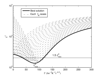
Figure 5: $\Gamma\sim L^{2}$ profile fit to the observations. Each dashed curve represents a roughness fraction $f_{\rm R}$ in the range of $0.0\sim 1.0$. The heavy line is a cubic spline interpolation curve for each lowest $L^{2}$ derived from each free parameter.

Table 9: Derived properties of 1996 FG3 from ATPM.

Property	Result
Thermal inertia $\Gamma$($\rm~{}Jm^{-2}s^{-0.5}K^{-1}$)	$80\pm 40$
Roughness fraction $f_{\rm R}$	$0.8^{+0.2}_{-0.4}$
Geometric albedo $p_{v}$	$0.045\pm 0.002$
Effective diameter $D_{\rm eff}$( km)	$1.69^{+0.05}_{-0.02}$
Primary diameter $D_{1}$( km)	$1.63^{+0.04}_{-0.03}$
Secondary diameter $D_{2}$( km)	$0.45^{+0.04}_{-0.03}$

In the following section, we will then utilize the above derived parameters to evaluate the surface thermal environment of 1996 FG3 at its aphelion and perihelion respectively.

5 Surface Thermal Environment

5.1 Temperature Distribution

On the basis of the derived shape model from the observations, the physical parameters in Table 7, and the thermal inertia determined from the ATPM fitting process, we attempt to simulate the temperature variation of 1996 FG3 over a rotation period. In Figures 6 and 7, we show the equatorial temperature and global surface temperature distribution for the primary at aphelion and perihelion, respectively.

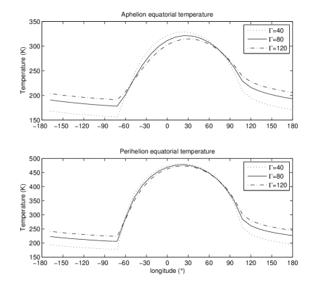
Figure 6: Equatorial temperature distribution of 1996 FG3 at aphelion and perihelion, respectively. Maximum temperature at $24^{\circ}$, minimum temperature at $-72^{\circ}$. ($0^{\circ}$ is the sub-solar point.)

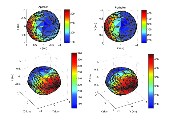
Figure 7: Global surface temperature distribution obtained from ATPM at the aphelion and perihelion, respectively. The color bar indicates the range of temperature, where red for high temperature and blue for low temperature.

Figure 6 shows the equatorial temperature distribution of 1996 FG3 at its aphelion and perihelion respectively. The maximum temperature does not appear at the solar point, but delays about $24^{\circ}$, and the minimum temperature occurs just a little after the local sunrise, delaying about $18^{\circ}$. Such delay effect between absorption and emission is actually caused by the non-zero thermal inertia and the finite rotation speed of the asteroid. On the other hand, according to Figure 6, the equatorial temperature of 1996 FG3 may range from $180$ to $480\rm~{}K$ over a whole orbit period.

Figure 7 shows the global surface temperature distribution of 1996 FG3 at its aphelion (left) and perihelion (right) respectively. In this figure, z-axis represents the asteroid’s spin axis, and x-axis points to the Sun in the framework of an asteroid center body-fixed coordinate system. The profile of temperature in Figure 7 is shown by the index of color-bar, and the red region represents the facets are sunlit, while the blue facets are referred to relatively low temperature.

5.2 Regolith

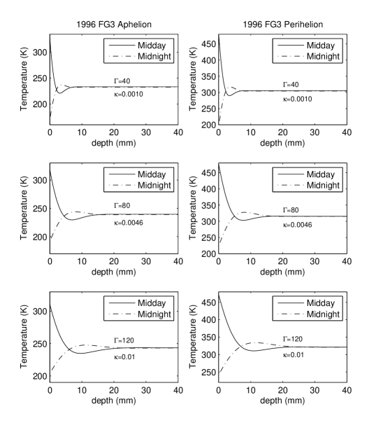
Figure 8: Temperature distribution of sub-surface on the equator of 1996 FG3 at local midday and midnight.

As mentioned previously, 1996 FG3 is chosen to be a backup target for MarcoPolo-R sample return mission. Hence, we still show great interest in the surface feature of the asteroid whether there exists a regolith layer on its surface. Apparently, thermal inertia is associated with the surface properties, where it will be helpful to infer the presence or absence of loose material on the surface. As known to all, fine dust has a very low thermal inertia about $30\rm~{}Jm^{-2}s^{-0.5}K^{-1}$, lunar regolith owns a relatively low value about $50\rm~{}Jm^{-2}s^{-0.5}K^{-1}$, a sandy regolith like Eros’ soil bears a value of $100-200\rm~{}Jm^{-2}s^{-0.5}K^{-1}$, but coarse sand occupies a higher thermal inertia profile $\sim$ $400\rm~{}Jm^{-2}s^{-0.5}K^{-1}$ (e.g., Itokawa’s Muses-Sea Regio). In comparison with the above materials, bare rock has an extremely higher thermal inertia more than $2500\rm~{}Jm^{-2}s^{-0.5}K^{-1}$ (Delbo et al., 2007). In this work, the thermal inertia of 1996 FG3 is estimated to be $80\pm 40\rm~{}Jm^{-2}s^{-0.5}K^{-1}$. Consequently, it is quite natural for one to suppose that the surface of 1996 FG3 may be covered by loose materials, perhaps a mixture of dust, fragmentary rocky debris and sand. In other word, there may exist a regolith layer on the surface of 1996 FG3, according to the above derived thermal inertia.

Theoretically, the so-called ”skin depth”:

$$l_{s}=\sqrt{\frac{\kappa}{\rho c\omega}}$$ (21)

is usually used to characterize the grain size of regolith. According to the definition of thermal inertia $\Gamma=\sqrt{\rho c\kappa}$. The profiles of mass density $\rho$, thermal conductivity $\kappa$, and specific heat capacity $c$ may be estimated from the above derived thermal inertia. Since the thermal conductivity $\kappa$ depends on particle size and temperature much more than $\rho$ and $c$, we attempt to assume a constant value for $\rho$ and $c$, and then estimate $\kappa$ from the above derived thermal inertia. Next, the estimation of skin depth will be easily acquired. Scheirich & Pravec (2009) has derived the mass density to be $1.4^{+1.5}_{-0.6}$ g cm^-3. Since the above derived value $\Gamma=80\pm 40\rm~{}Jm^{-2}s^{-0.5}K^{-1}$ is similar to that of the Moon despite a little higher, we assume the specific heat capacity of 1996 FG3 is similar to that of the Moon, about $1000\rm~{}Jkg^{-1}K^{-1}$. Then the thermal conductivity $\kappa$ is estimated to be $0.001\sim 0.01\rm~{}Jkg^{-1}K^{-1}$ and $l_{s}$ is $1.3\sim 3.9\rm~{}mm$. Such small $\kappa$ and $l_{s}$ obviously support the possible existence of loose material or regolith over the surface of 1996 FG3. However, the depth of the regolith layer, covered on the asteroid’s surface, attracts our great attention.

We carried out simulations to explore the regolith depth versus temperature distribution of sub-surface for $\Gamma=40$, $80$ and $120\rm~{}Jm^{-2}s^{-0.5}K^{-1}$, respectively (see Figure 8). The left panels show the results are obtained when the asteroid moves at aphelion, while the right panels exhibit those at perihelion. In each panel, two profiles, which are respectively, plotted by solid line (local midday) and dashed line (local midnight), show that the sub-surface temperature changes with the depth (the distance from the surface). In these panels, the temperature goes down as the depth increases at local noon, while it goes up as the depth increases at local midnight until a certain depth, where two curves are overlapped. This phenomenon results from the internal boundary equation 4. The figure shows the temperature distribution of the very loose regolith layer, the thermal conductivity of which may be in the range of $0.001\sim 0.01\rm~{}Jkg^{-1}K^{-1}$. And the minimum depth of this layer may be estimated from Figure 8. Herein the regolith depth of the very surface of 1996 FG3 is reckoned to be $5\sim 20\rm~{}mm$. This minimum value of regolith depth may be considered as a reference for the design of a spacecraft if a lander is equipped. On the other hand, the existence of regolith over the surface of the primary of 1996 FG3 actually does good to a sample return mission.

6 Discussion and Conclusion

In this work, we have derived a new 3D convex shape model of the primary of 1996 FG3 from the published lightcurves, where the best-fit orientation of its spin axis is determined to be $\lambda=237.7^{\circ}$ and $\beta=-83.8^{\circ}$, with a rotation period of $\sim$ 3.5935 h. On the basis of the numerical codes independently developed according to thermophysical model, we apply the shape model and the required input physical parameters to fit three sets of mid-infrared measurements for 1996 FG3. Herein we summarize the major physical properties obtained for the asteroid as follows: the geometric albedo and effective diameter are, respectively, $p_{v}=0.045\pm 0.002$ and $D_{\rm eff}=1.69^{+0.05}_{-0.02}\rm~{}km$; the diameters of the primary and secondary are calculated to be $D_{1}=1.63^{+0.04}_{-0.03}\rm~{}km$ and $D_{2}=0.45^{+0.04}_{-0.03}\rm~{}km$, respectively. Moreover, the thermal inertia $\Gamma$ is also determined to be a low value of $80\pm 40\rm~{}Jm^{-2}s^{-0.5}K^{-1}$, whereas the roughness fraction $f_{\rm R}$ is estimated to be $0.8^{+0.2}_{-0.4}$.

From the simulations, we find that low thermal inertia ($<100\rm~{}Jm^{-2}s^{-0.5}K^{-1}$) would make a perfect fitting to the VISIR observations on 19 January, 2011 (with respect to a low phase angle), whereas the observations obtained at higher phase angles (Table 3 and 4) are very sensitive to $f_{\rm R}$, thereby leading to a best-fit solution with the case of large roughness fraction. Given that we simultaneously perform the computation using the combination data (Tables 3,4 and 5), a broad range of $L^{2}$ profiles are obtained in the fitting. Furthermore, to acquire a significant uncertainty for the outcomes, we finally choose a $50\%$ range of the minimum $L^{2}$ to determine the best-fit solution for thermal inertia of 1996 FG3. On the other hand, via the simultaneous fitting with these observations at different solar phase angles, the degeneracy of solutions between thermal inertia and roughness is removed, making it capable to determine the estimation for thermal inertia and roughness separately. The ratio of ”observation/model” (see Figures 9 and 10) is a good indicator that examines how the results from the model match the observations at various phase angles and wavelengths (M$\ddot{u}$ller et al., 2005, 2011, 2012). Hence, this enables us to conclude that the fitting process is correct and the derived results are reliable.

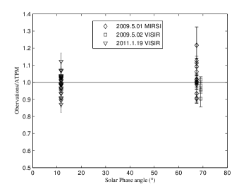
Figure 9: The observation/ATPM ratios as a function of phase angle for $f_{\rm R}=0.8$, $\Gamma=80\rm~{}Jm^{-2}s^{-0.5}K^{-1}$, and $D_{\rm eff}=1.69\rm~{}km$.

Figure 10: The observation/ATPM ratios as a function of wavelength for $f_{\rm R}=0.8$, $\Gamma=80\rm~{}Jm^{-2}s^{-0.5}K^{-1}$, and $D_{\rm eff}=1.69\rm~{}km$.

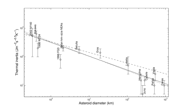
Figure 11: Thermal inertia versus the size of asteroids (Delbo et al., 2007). The value of 1996 FG3 derived in this work is also labeled.

According to the ATPM fitting results shown in Table 9, the evaluated large roughness fraction $f_{\rm R}=0.8^{+0.2}_{-0.4}$ for 1996 FG3 may suggest a rough surface on the asteroid. However, the asteroid’s mean surface thermal inertia is estimated to be a relative low value. Then the question arises – why this asteroid bears such a low thermal inertia with a very rough surface. As the adopted roughness model in the ATPM is assumed to be an irregularity degree of a surface at scales smaller than the global shape model resolution (like a facet area) but larger than the thermal skin depth. Therefore, 1996 FG3 would be likely to have a rough surface, which may or may not include craters of any size, and a porous or dusty material. The recent work of Perna et al. (2013) suggested the surface of 1996 FG3 may be a compact one, with the existence of regions showing different roughness, similar to that of Itokawa. Hence, there would be possible for an asteroid to possess a large roughness fraction and low thermal inertia.

However, the NEA binaries may have a high averaged thermal inertia of $\Gamma\approx 480\pm 70\rm~{}Jm^{-2}s^{-0.5}K^{-1}$ (Delbo et al., 2011), indicating that high thermal inertia could be supportive to the binary formation scenario due to YORP mechanism. In this work, we have derived thermal inertia $\Gamma=80\pm 40\rm~{}Jm^{-2}s^{-0.5}K^{-1}$ for 1996 FG3, and it appears below their estimation. Nevertheless, it is still likely for a rubble-pile asteroid to have a low thermal inertia , thereby remaining a rough surface during a long dynamical evolution due to space-weathering and regolith migration. In this sense, the binary 1996 FG3 may also be produced via the YORP rotation acceleration effect at a very earlier time, but retain a roughness surface from then, resulting in the distribution of a great many meter-size (or even smaller) craters on the surface. Thus, these tiny craters might be covered or surrounded by loose materials, making it appear a low thermal inertia.

Delbo et al. (2007) showed that the average thermal inertia for NEAs may be $\Gamma=200\pm 40\rm~{}Jm^{-2}s^{-0.5}K^{-1}$. Figure 11 exhibits the variation of mean thermal inertia with the size of asteroids from the observations. From this figure, we observe that the value of thermal inertia for 1996 FG3 given in this work (labeled in red) deviates a little from the prediction profile. In addition, our outcome for the binary system is a bit lower than that of Wolters et al. (2011). This results from that we perform the combination fitting with additional thermal-IR observations (Tables 3 and 4), which may provide new insight for the thermal study of binary asteroids.

In conclusion, the surface of 1996 FG3’s primary may be a very rough surface, on which loose materials such as fine dust, fragmentary rocky debris, sands or most likely a stuff of their mixture are covered, composing a kind of regolith. The depth of the possible regolith layer is evaluated to be approximately $5\sim 20\rm~{}mm$. Such implication may provide substantial information for engineering of the sample return mission, for example, a selection of landing area. However, we should place special emphasis on that this estimation is simply a roughly minimum value of the regolith layer over the very surface of the asteroid rather than a sort of megaregolith below the layer. Since the thermal conductivity $\kappa$ of the megaregolith has a complicated relationship with the depth below the surface (Haack et al, 1990), thereby we cannot simulate the temperature distribution accurately from a one-dimension thermophysical model. On the other hand, the formation mechanism for 1996 FG3 is still a mystery, which the YORP acceleration mechanism may play a role in producing its shape and orbital configuration (Walsh et al., 2008). In short, the investigations by future space missions will throw new light on the formation scenario for this asteroid.

References

- Barucci et al. (2012) Barucci, M. A., Cheng, A. F., Michel, P., et al. 2012, Experimental Astronomy, 33, 645
- Benner et al. (2012) Benner, L.A., et al. 2012, Asteroids, Comets, Meteors, 6403
- Binzel et al. (2001) Binzel, R. P., Harris, A. W., Bus, S. J., & Burbine, T. H. 2001, Icarus, 151, 139
- Binzel et al. (2012) Binzel, R. P., Polishook, D., DeMeo, F. E., Emery, J. P., & Rivkin, A. S. 2012, Lunar and Planetary Institute Science Conference Abstracts, 43, 2222
- Bowell et al. (1989) Bowell, E., Hapke, B., Domingue, D., Lumme, K., Peltoniemi, J. & Harris, A.W. 1989, Application of photometric models to asteroids. In Asteroids II, pp. 524-556
- Christou (2003) Christou, A. A., 2003, Planet. Space Sci., 51, 221
- Delbo & Harris (2002) Delbo, M., & Harris, A.W., 2002, Meteoritics & Planetary Science, 37, 1929-1936
- Delbo et al. (2007) Delbo, M., Oro, A., Harris, A.W., Mottola, S., & Muller, M., 2007, Icarus, 190, 236-249
- Delbo et al. (2011) Delbo, M., Walsh, K., Mueller, M., Harris, A.W., & Howell, E.S., 2011, Icarus, 212, 138
- de León et al. (2011) de León, J., Mothé-Diniz, T., Licandro, J., Pinilla-Alonso, N., & Campins, H., 2011, A&A, 530, L12
- de León et al. (2013) de León, J., Lorenzi, V., Alí-Lagoa, V., et al. 2013, A&A, 556, A33
- Durech et al. (2010) Durech, J., Sidorin, V., & Kaasalainen, M., 2010, A&A, 513, A46
- Fowler & Chillemi (1992) Fowler, J.W., & Chillemi, J.R., 1992, IRAS asteroids data processing. In The IRAS Minor Planet Survey, pp.17-43
- Haack et al (1990) Haack, H., Rasmussen, K. L., Warren, P. H., 1990, JGR, 95, 5111
- Harris (1989) Harris, A.W. et al., 1989, Icarus, 77, 171
- Harris (1998) Harris, A.W., 1998, Icarus, 131, 291-301
- Kaasalainen & Torppa (2001) Kaasalainen M. & Torppa J., 2001, Icarus, 153, 24
- Kaasalainen et al. (2001) Kaasalainen M., Torppa, J., & Muinonen, K., 2001, Icarus, 153, 37
- Lagerros (1996) Lagerros, J.S.V., 1996, A&A, 310, 1011-1020
- Lowry et al. (2012) Lowry, S. et al., 2012, A&A, 548, A12
- Mottola & Lahulla (2000) Mottola, S., & Lahulla, F., 2000, Icarus, 146, 556
- Mller et al. (2005) Mller, T.G., Sekiguchi, T., Kaasalainen, M., Abe, M., & Hasegawa, S., 2005, A&A, 443, 347
- Mller et al. (2011) Mller, T.G., Durech, J., Hasegawa, S., et al., 2011, A&A, 525, A145
- Mller et al. (2012) Mller, T.G., O’Rourke, L., Barucci, A.M., et al., 2012, A&A, 548, A36
- Mueller et al. (2011) Mueller, M., Delbo, M. Hora, J., et al., 2011, AJ, 141, 109
- Perna et al. (2013) Perna, D., Dotto, E.A.B., Fornasier, S., et al., 2013, A&A, 555, A62
- Perozzi et al. (2001) Perozzi, E., Rossi, A., & Valsecchi, G. B., 2001, Planet. Space Sci., 49, 3
- Pravec et al. (1996) Pravec, P., Sarounova, L., Wolf, M., 1996, Icarus, 124, 471
- Pravec et al. (1997) Pravec, P., & Hahn, G., 1997, Icarus, 127, 431
- Pravec et al. (1998) Pravec, P.,Wolf, M., Sarounova, L., 1998, Icarus, 133, 79
- Pravec et al. (2000) Pravec, P., Sarounova, L., Rabinowitz, D.L., et al., 2000, Icarus, 146, 190
- Pravec et al. (2006) Pravec, P., Scheirich, P., Kusnirak, P., et al., 2006, Icarus, 181, 63
- Press et al. (1992) Press, W. H., Teukolsky, S. A., Vetterling, W. T., & Flannery, B. P. 1992, Numerical Recipes in C, 2nd ed., Cambridge: University Press
- Rivkin et al. (2013) Rivkin, A. S., Howell, E. S., Vervack, R. J., et al. 2013, Icarus, 223, 493
- Rozitis & Green (2011) Rozitis, B., & Green, S.F., 2011, MNRAS, 415, 2042
- Rozitis & Green (2012) Rozitis, B., & Green, S.F., 2012, MNRAS, 423, 367
- Scheirich & Pravec (2009) Scheirich, P., & Pravec, P., 2009, Icarus, 200, 531
- Spencer & Lebofsky (1989) Spencer, J.R., Lebofsky, L.A., & Sykes, M.V., 1989, Icarus, 78, 337
- Walsh et al. (2012) Walsh, K.J., Delbo, M., Mueller, M., Binzel, R.P., & Demeo, F.E., 2012, ApJ, 748, 104
- Walsh et al. (2008) Walsh, K.J., Richardson, D.C., & Michel, P., 2008, Nature, 454, 188
- Wolters et al. (2011) Wolters, S.D., Rozitis, B., Duddy, S.R., et al., 2011, MNRAS, 418, 1246