Non-Termination Analysis of Java Bytecode

Abstract

We introduce a fully automated static analysis that takes a sequential Java bytecode program $P$ as input and attempts to prove that there exists an infinite execution of $P$. The technique consists in compiling $P$ into a constraint logic program $P_{\mathit{CLP}}$ and in proving non-termination of $P_{\mathit{CLP}}$; when $P$ consists of instructions that are exactly compiled into constraints, the non-termination of $P_{\mathit{CLP}}$ entails that of $P$. Our approach can handle method calls; to the best of our knowledge, it is the first static approach for Java bytecode able to prove the existence of infinite recursions. We have implemented our technique inside the Julia analyser. We have compared the results of Julia on a set of 113 programs with those provided by AProVE and Invel, the only freely usable non-termination analysers comparable to ours that we are aware of. Only Julia could detect non-termination due to infinite recursion.

1 Introduction

In this paper, we address the issue of automatically proving non-termination of sequential Java bytecode programs. We describe and implement a static analysis that takes a program $P$ as input and attempts to prove that there exists an infinite execution of $P$. It is well-known that termination of computer programs is an undecidable property, hence a non-termination analyser for Java bytecode can be used to complement any existing termination analyser, e.g., AProVE [18], COSTA [1] or Julia [28]. Research in non-termination has mainly been focused on logic programs [6, 11, 20, 21, 26, 27] and term rewriting systems [14, 19, 31, 32, 34, 35]. Only a few recent papers address the problem of proving non-termination of imperative programs: [8] considers Java bytecode, [15] considers programs written in the C language and [30] considers imperative programs that can be described as logical formulæ written in a simple while-language.

1.1 Contributions

In [22], we presented a first experimentation with the automatic derivation of non-termination proofs for Java bytecode programs. There, we started from the results introduced in a preliminary version of [28] where the original Java bytecode program $P$ is translated into a constraint logic program $P_{\mathit{CLP}}$ whose termination entails that of $P$. We had the idea of carrying out a very simple non-termination analysis of $P_{\mathit{CLP}}$ using earlier results introduced in [20]. During our experiments with non-terminating Java bytecode programs, we made the empirical observation that the non-termination of $P_{\mathit{CLP}}$ entails that of $P$ when $P_{\mathit{CLP}}$ is an exact translation of $P$. We only introduced a very intuitive and non-formal definition of exactness and we did not give any formal proof of this entailment. In this paper, we provide the formal definitions and results that are missing in [22]; the corresponding formal proofs are available in the long version at [23]. We also provide a non-termination criterion that works for method calls and recursion, together with a new experimental evaluation of our results over a set of 113 Java bytecode programs.

The technique we apply for proving non-termination of $P_{\mathit{CLP}}$ is an improvement of a simple sufficient condition for linear binary CLP programs [20]. This improved condition (Proposition 4) is another contribution of this paper. Our main result (Theorem 2) is independent of the non-termination detection procedure. Let us point out that there is no perfect non-termination criterion for the CLP programs we consider: [7] shows that the termination of binary CLP programs with linear constraints over the integers is undecidable. However some interesting subclasses have been recently investigated. For instance, when all the constraints are of the form $x>y$ or $x\geq y$, termination of the binary CLP program is decidable [5]. So when the generated CLP program falls into this class, we could replace our general non-termination test by a decision procedure for non-termination.

Our results are fully implemented inside the Julia static analyser, that we used for conducting the experiments. Julia is a commercial product (http://www.juliasoft.com). Its non-termination analysis can be freely used through the web interface [17], whose power is limited by a time-out and a maximal size of analysis.

1.2 Related Works

To the best of our knowledge, only [8, 15, 30] introduce methods and implementations that are directly comparable to the results of this paper.

In [8], the program $P$ under analysis is first transformed into a termination graph that finitely represents all runs through the program. Then, a term rewrite system is generated from the graph and existing techniques from term rewriting are used to prove non-termination of the rewrite system. This approach has been successfully implemented inside the AProVE analyser [2, 13]. Note that the rewrite system generated from the termination graph is an abstraction [10] of $P$; the technique that we present in this paper also computes an abstraction of $P$ but a difference is that our abstraction consists of a constraint logic program $P_{\mathit{CLP}}$ instead of a term rewrite system.

The technique described in [15] is a combination of dynamic and static analysis. It consists in generating lassos that are checked for feasibility. A lasso consists of a finite program path called stem, followed by a finite program path called loop; it is feasible when an execution of the stem can be followed by infinitely many executions of the loop. Lassos are generated through a dynamic execution of the program on concrete as well as symbolic inputs; symbolic constraints are gathered during this execution and are used for expressing the feasibility of the lassos as a constraint satisfaction problem. This technique has been implemented inside the TNT non-termination analyser for C programs. The analysis that we present in this paper also looks for feasible lassos: it tries to detect some loops that have an infinite execution from some input values and to prove that these values are reachable from the main entry point of the program (Proposition 5). A difference is that our technique does not combine static with dynamic analysis. Another difference is that the approach of [15] provides a bit-level analysis which is able to detect non-termination due, e.g., to arithmetic overflow.

In [30], the authors consider a simple while-language that is used to describe programs as logical formulæ. The non-termination of the program $P$ under analysis is expressed as a logical formula involving the description of $P$. The method then consists in proving that the non-termination formula is true by constructing a proof tree using a Gentzen-style sequent calculus. The rule of the sequent calculus corresponding to the while instruction uses invariants, that have to be generated by an external method. Hence, [30] introduces several techniques for creating and for scoring the invariants according to their probable usefulness; useless invariants are discarded (invariant filtering). The generated invariants are stored inside a queue ordered by the scores. The algorithms described in [30] have been implemented inside the Invel non-termination analyser for Java programs [16]. Invel uses the KeY [4] theorem prover for constructing proof trees. As far as we know, it was the first tool for automatically proving non-termination of imperative programs.

One of the main differences between the techniques introduced in [15, 30] and ours is that we first construct an abstraction of the program under analysis and then we keep on reasoning on this abstraction only. The algorithms presented in [15, 30] model the semantics of the concrete program more accurately. They hence do not suffer from some lack of precision that we face; we were not able to exactly translate some bytecode instructions into constraints, therefore our method fails on the programs that include these instructions. On the other hand, the techniques that directly consider the original concrete program are generally time consuming and they do not scale very well.

Finally, a major difference between our approach and that of [8, 30] is that we are able to detect non-termination due to infinite recursion, whereas [8, 30] are not. Our experiments illustrate this consideration very clearly. Note that the approach in [15] can deal with non-terminating recursion.

1.3 Organisation of this Paper

The rest of this paper is organised as follows. Section 2 introduces the basic formal material borrowed from [28]. Section 3 provides a formal definition of exactness for the abstraction of a Java bytecode instruction into a linear constraint. In Section 4, we show how to automatically generate a constraint logic program $P_{\mathit{CLP}}$ from a Java bytecode program $P$ so that the non-termination of $P_{\mathit{CLP}}$ entails that of $P$. Section 5 deals with proving non-termination of $P_{\mathit{CLP}}$; it provides an improvement of a non-termination criterion that we proposed in [20]. Section 6 describes our experiments on a set of 113 non-terminating programs obtained from different sources. Section 7 concludes the paper.

2 Preliminaries

We strictly adhere to the notations, definitions, and results introduced in [28]. We briefly list the elements that are relevant to this paper.

For ease of exposition, we consider a simplification of the Java bytecode where values can only be integers, locations or null.

Definition 1.

The set of values is $\mathbb{Z}\cup\mathbb{L}\cup\{\mathtt{null}\}$, where $\mathbb{Z}$ is the set of integers and $\mathbb{L}$ is the set of memory locations. A state of the Java Virtual Machine is a triple $\langle l\operatorname{\mid\!\mid}s\operatorname{\mid\!\mid}\mu\rangle$ where $l$ is an array of values, called local variables and numbered from $0$ upwards, $s$ is a stack of values, called operand stack (in the following, just stack), which grows leftwards, and $\mu$ is a memory, or heap, which maps locations into objects. An object is a function that maps its fields into values. We write $l^{k}$ for the value of the $k$th local variable; we write $s^{k}$ for the value of the $k$th stack element ($s^{0}$ is the base of the stack, $s^{1}$ is the element above and so on). The set of all states is denoted by $\Sigma$. When we want to fix the exact number $\#l\in{\rm Nature}$ of local variables and $\#s\in{\rm Nature}$ of stack elements allowed in a state, we write $\Sigma_{\#l,\#s}$. ∎

Example 1.

Consider a memory

$$\mu=[\ell_{1}\mapsto o_{1},\ell_{2}\mapsto o_{2},\ell_{3}\mapsto o_{3},\ell_{4}\mapsto o_{4},\ell_{5}\mapsto o_{5}]$$

where $o_{1}=[f\mapsto\ell_{4}]$, $o_{2}=[f\mapsto\mathtt{null}]$, $o_{3}=[f\mapsto\ell_{5}]$, $o_{4}=[f\mapsto\mathtt{null}]$ and $o_{5}=[f\mapsto\mathtt{null}]$. Then,

$$\sigma=\langle[5,\ell_{2}]\operatorname{\mid\!\mid}\ell_{1}::\ell_{2}::\ell_{3}\operatorname{\mid\!\mid}\mu\rangle$$

is a state in $\Sigma_{2,3}$. Here, $\ell_{1}$ is the topmost element of the stack of $\sigma$, $\ell_{2}$ is the underlying element and $\ell_{3}$ is the element still below it. ∎

Definition 2.

The set of types of our simplified Java Virtual Machine is $\mathbb{T}=\mathbb{K}\cup\{\mathtt{int},\mathtt{void}\}$, where $\mathbb{K}$ is the set of all classes. The $\mathtt{void}$ type can only be used as the return type of methods. A method signature is denoted by $\kappa.m(t_{1},\ldots,t_{p}):t$ standing for a method named $m$, defined in class $\kappa$, expecting $p$ explicit parameters of type, respectively, $t_{1},\ldots,t_{p}$ and returning a value of type $t$, or returning no value when $t=\mathtt{void}$.∎

We recall that in object-oriented languages, a non-static method $\kappa.m(t_{1},\ldots,t_{p}):t$ has also an implicit parameter of type $\kappa$ called this inside the code of the method. Hence, the actual number of parameters is $p+1$.

A restricted set of eleven Java bytecode instructions is considered in [28]. These instructions exemplify the operations that the Java Virtual Machine performs. Similarly, in this paper we only consider nine instructions, but our implementation handles most of their variants.

Definition 3.

We let $\mathcal{C}$ denote the set consisting of the following Java bytecode instructions.

• $\mathsf{const}\ c$, pushes the constant $c$ on top of the stack.

• $\mathsf{dup}$, duplicates the topmost element of the stack.

• $\mathsf{new}\ \kappa$, creates an object of class $\kappa$ and pushes a reference to it on the stack.

• $\mathsf{load}\ i$, pushes the value of local variable $i$ on top of the stack.

• $\mathsf{store}\ i$, pops the top value from the stack and writes it into local variable $i$.

• $\mathsf{add}$, pops the topmost two values from the stack and pushes their sum instead.

• $\mathsf{putfield}\ f$, where $f$ has integer type, pops the topmost two values $v$ (the top) and $\ell$ (under $v$) from the stack where $\ell$ must be a reference to an object $o$ or $\mathtt{null}$; if $\ell$ is $\mathtt{null}$, the computation stops, else $v$ is stored into field $f$ of $o$.

• $\mathsf{ifeq\ of\ type}\ t$, with $t\in\mathbb{K}\cup\{\mathtt{int}\}$, pops the topmost element from the stack and checks if it is 0 (when $t$ is $\mathtt{int}$) or $\mathtt{null}$ (when $t$ is a class); if it is not the case, the computation stops.

• $\mathsf{if}\mathit{\langle{}cond\rangle}\mathsf{\ of\ type}\ \mathtt{int}$, with $\mathit{cond}\in\{\mathsf{lt},\mathsf{le},\mathsf{gt},\mathsf{ge}\}$, pops the topmost element from the stack and checks, respectively, if it is less than 0, less than or equal to 0, greater than 0, greater than or equal to 0; if it is not the case, the computation stops.

• $\mathsf{call}\ \kappa.m(t_{1},\ldots,t_{p}):t$. If $m$ is a static method, this instruction pops the topmost $p$ values (the actual parameters) $a_{1}$, …, $a_{p}$ from the stack (where $a_{p}$ is the topmost value) and $m$ is run from a state having an empty stack and a set of local variables bound to $a_{1},\ldots,a_{p}$. If $m$ is not static, this instruction pops the topmost $p+1$ values (the actual parameters) $a_{0}$, $a_{1}$, …, $a_{p}$ from the stack (where $a_{p}$ is the topmost value). Value $a_{0}$ is called receiver of the call and must be $\mathtt{null}$ or a reference to an object of class $\kappa$ or of a subclass of $\kappa$. If the receiver is $\mathtt{null}$, the computation stops. Otherwise, method $m$ is run from a state having an empty stack and a set of local variables bound to $a_{0},a_{1},\ldots,a_{p}$.∎

Unlike [28], we do not consider the instruction $\mathsf{getfield}\ f$, which is used for getting the value of the field $f$ of an object, and $\mathsf{putfield}\ f$, where $f$ has class type. This is because we cannot design an exact abstraction, as defined in Sect. 3, of these instructions. We also do not consider the instruction $\mathsf{ifne\ of\ type}\ t$, which pops the topmost element from the stack, checks if it is 0 (when $t$ is int) or null (when $t$ is a class) and, if it is the case, stops the computation. This is because we have implemented the results of this paper inside the Julia analyser, which now systematically replaces the $\mathsf{ifne}$ instruction with a disjunction of $\mathsf{iflt}$ (less than 0) and $\mathsf{ifgt}$ (greater than 0); these two instructions belong to the set considered by our implementation. Finally, the $\mathsf{call}$ instruction considered in [28] has the form

$$\mathsf{call}\ \kappa_{1}.m(t_{1},\ldots,t_{p}):t,\ldots,\kappa_{n}.m(t_{1},\ldots,t_{p}):t$$

where $S=\{\kappa_{1}.m(t_{1},\ldots,t_{p}):t,\ldots,\kappa_{n}.m(t_{1},\ldots,t_{p}):t\}$ is an over-approximation of the set of methods that might be called at run-time, at the program point where the call occurs. This is because object-oriented languages, such as Java bytecode, allow dynamic lookup of method implementations in method calls, on the basis of the run-time class of their receiver. Hence, the exact control-flow graph of a program is not computable in general, but an over-approximation can be computed instead. In this paper, we present a technique for proving existential non-termination i.e., for proving that there exists some inputs that lead to an infinite execution. So, we have to ensure that the methods we consider in the $\mathsf{call}$ instructions are effectively called at run-time: this happens when $S$ only consists of one element. Therefore, unlike [28], we only consider calls of the form $\mathsf{call}\ \kappa.m(t_{1},\ldots,t_{p}):t$ in this paper, and our technique cannot deal with situations where $S$ consists of more than one element.

We assume that flat code, as the one in Fig. 1, is given a structure in terms of blocks of code linked by arrows expressing how the flow of control passes from one to another. We require that a $\mathsf{call}$ instruction can only occur at the beginning of a block. For instance, Fig. 2 shows the blocks derived from the code of the method sum in Fig. 1. Note that at the beginning of the methods, the local variables hold the parameters of the method.

From now on, a Java bytecode program will be a graph of blocks, such as that in Fig. 2; inside each block, there is one or more instructions among those described in Definition 3. This graph typically contains many disjoint subgraphs, each corresponding to a different method or constructor. The ends of a method or constructor, where the control flow returns to the caller, are the end of every block with no successor, such as the leftmost one in Fig. 2. For simplicity, we assume that the stack there contains exactly as many elements as are needed to hold the return value (normally $1$ element, but $0$ element in the case of methods returning $\mathtt{void}$, such as all the constructors or the main method).

A denotational semantics for Java bytecode is presented in [28] together with a path-length relational abstract domain that is used for proving termination of Java bytecode programs. Denotations are state transformers that can be composed to model the sequential execution of instructions.

Definition 4.

A denotation is a partial function $\Sigma\to\Sigma$ from an input state to an output or final state. The set of denotations is denoted by $\Delta$. When we want to fix the number of local variables and stack elements in the input and output states, we write $\Delta_{l_{i},s_{i}\to l_{o},s_{o}}$, standing for $\Sigma_{l_{i},s_{i}}\to\Sigma_{l_{o},s_{o}}$. Let $\delta_{1},\delta_{2}\in\Delta$. Their sequential composition is $\delta_{1};\delta_{2}=\lambda\sigma.\delta_{2}(\delta_{1}(\sigma))$, which is undefined when $\delta_{1}(\sigma)$ is undefined or when $\delta_{2}(\delta_{1}(\sigma))$ is undefined. ∎

For each instruction $\mathsf{ins}$ in $\mathcal{C}$ and program point $q$ where $\mathsf{ins}$ occurs, [28] provides the definition of a corresponding denotation $\mathit{ins}_{q}$.

Example 2.

Let $q$ be a program point where the instruction $\mathsf{dup}$ occurs and let $\#l$ and $\#s$ be the number of local variables and stack elements at $q$. The denotation $\mathit{dup}_{q}$ corresponding to $\mathsf{dup}$ at $q$ is defined as: $\mathit{dup}_{q}\in\Delta_{\#l,\#s\to\#l,\#s+1}$ and $\mathit{dup}_{q}=\lambda\langle l\operatorname{\mid\!\mid}\mathit{top}::s\operatorname{\mid\!\mid}\mu\rangle.\langle l\operatorname{\mid\!\mid}\mathit{top}::\mathit{top}::s\operatorname{\mid\!\mid}\mu\rangle$ where $\mathit{top}::s$ denotes a non-empty stack whose top element is $\mathit{top}$ and remaining portion is $s$. ∎

[28] also defines the abstraction of $\mathit{ins}_{q}$ into its path-length polyhedron $\mathit{ins}^{\mathbb{PL}}_{q}$.

Definition 5.

Let $l_{i},s_{i},l_{o},s_{o}\in{\rm Nature}$. The set $\mathbb{PL}_{l_{i},s_{i}\to l_{o},s_{o}}$ of the path-length polyhedra contains all finite sets of integer linear constraints over the variables $\{\check{{l}}^{k}\mid 0\leq k<l_{i}\}\cup\{\check{{s}}^{k}\mid 0\leq k<s_{i}\}\cup\{\hat{{l}}^{k}\mid 0\leq k<l_{o}\}\cup\{\hat{{s}}^{k}\mid 0\leq k<s_{o}\}$, using only the $\leq$, $\geq$ and $=$ comparison operators. ∎

The path-length polyhedron $\mathit{ins}_{q}^{\mathbb{PL}}$ describes the relationship between the sizes $\check{{l}}^{k}$ and $\check{{s}}^{k}$ of the local variables and stack elements in the input state of $\mathit{ins}_{q}$ and the sizes $\hat{{l}}^{k}$ and $\hat{{s}}^{k}$ of the local variables and stack elements in the output state of $\mathit{ins}_{q}$. The size of a local variable or stack element $v$ in a memory $\mu$ is denoted by $\mathit{len}(v,\mu)$ and is informally defined as: if $v\in\mathbb{Z}$ then $\mathit{len}(v,\mu)=v$, if $v$ is null then $\mathit{len}(v,\mu)=0$ and if $v$ is a location then $\mathit{len}(v,\mu)$ is the maximal length in $\mu$ of a chain of locations that one can follow from $v$.

Example 3.

[28] defines $\mathit{dup}_{q}^{\mathbb{PL}}=\mathit{Unchanged}_{q}(\#l,\#s)\cup\{\check{{s}}^{\#s-1}=\hat{{s}}^{\#s}\}$ where $\mathit{Unchanged}_{q}(\#l,\#s)=\{\check{{l}}^{i}=\hat{{l}}^{i}\mid 0\leq i<\#l\}\cup\{\check{{s}}^{i}=\hat{{s}}^{i}\mid 0\leq i<\#s\}$. Hence, $\mathit{dup}_{q}^{\mathbb{PL}}$ expresses the fact that after an execution of $\mathsf{dup}$, the new top of the stack has the same path-length as the former one ($\{\check{{s}}^{\#s-1}=\hat{{s}}^{\#s}\}$) and that the path-length of the local variables and stack elements is unchanged ($\mathit{Unchanged}_{q}(\#l,\#s)$). ∎

Note that [28] also provides the definition of the abstract counterpart $;^{\mathbb{PL}}$ of the operator ; used for composing denotations. The operator $;^{\mathbb{PL}}$ is hence used for composing path-length polyhedra.

Definition 6.

Let $\mathit{\mathit{pl}}_{1}\in\mathbb{PL}_{l_{i},s_{i}\to l_{t},s_{t}}$ together with $\mathit{\mathit{pl}}_{2}\in\mathbb{PL}_{l_{t},s_{t}\to l_{o},s_{o}}$. Let $T=\{\overline{l}^{0},\ldots,\overline{l}^{l_{t}-1},\overline{s}^{0},\ldots,\overline{s}^{s_{t}-1}\}$. We define $\mathit{\mathit{pl}}_{1};^{\mathbb{PL}}\mathit{\mathit{pl}}_{2}\in\mathbb{PL}_{l_{i},s_{i}\to l_{o},s_{o}}$ as

$$\mathit{\mathit{pl}}_{1};^{\mathbb{PL}}\mathit{\mathit{pl}}_{2}=\exists_{T}\left(\mathit{\mathit{pl}}_{1}[\hat{{v}}\mapsto\overline{v}\mid\overline{v}\in T]\cup\mathit{\mathit{pl}}_{2}[\check{{v}}\mapsto\overline{v}\mid\overline{v}\in T]\right)$$

where $\mathit{\mathit{pl}}_{1}[\hat{{v}}\mapsto\overline{v}\mid\overline{v}\in T]$ (resp. $\mathit{\mathit{pl}}_{2}[\check{{v}}\mapsto\overline{v}\mid\overline{v}\in T]$) denotes the replacement in $\mathit{\mathit{pl}}_{1}$ (resp. $\mathit{\mathit{pl}}_{2}$) of $\hat{{v}}$ with $\overline{v}$ (resp. $\check{{v}}$ with $\overline{v}$). ∎

The abstractions $\mathit{ins}_{q}^{\mathbb{PL}}$, for each $\mathsf{ins}\in\mathcal{C}$, and the abstraction $;^{\mathbb{PL}}$ are all proved to be correct i.e., [28] provides the proof that these abstractions include their concrete counterpart in their concretisation.

Definition 7.

Let $\mathit{pl}\in\mathbb{PL}_{l_{i},s_{i}\to l_{o},s_{o}}$ and $\mathit{\rho}$ be an assignment from a superset of the variables of $\mathit{pl}$ into $\mathbb{Z}\cup\{+\infty\}$. We say that $\rho$ is a model of $\mathit{pl}$ and we write $\rho\models\mathit{pl}$ when $\rho(\mathit{pl})$ is true, that is, by substituting, in $\mathit{\mathit{pl}}$, the variables with their values provided by $\rho$, we get a tautological set of ground constraints. ∎

Any state can be mapped into an input path-length assignment, when it is considered as the input state of a denotation, or into an output path-length assignment, when it is considered as the output state of a denotation.

Definition 8.

Let $\langle l\operatorname{\mid\!\mid}s\operatorname{\mid\!\mid}\mu\rangle\in\Sigma_{\#l,\#s}$. Its input path-length assignment is

$$\check{{\mathit{len}}}(\langle l\operatorname{\mid\!\mid}s\operatorname{\mid\!\mid}\mu\rangle)= \;[\check{{l}}^{k}\mapsto\mathit{len}(l^{k},\mu)\mid 0\leq k<\#l]$$

$$\cup[\check{{s}}^{k}\mapsto\mathit{len}(s^{k},\mu)\mid 0\leq k<\#s]$$

and, similarly, its output path-length assignment is

$$\hat{{\mathit{len}}}(\langle l\operatorname{\mid\!\mid}s\operatorname{\mid\!\mid}\mu\rangle)= \;[\hat{{l}}^{k}\mapsto\mathit{len}(l^{k},\mu)\mid 0\leq k<\#l]$$

$$\cup[\hat{{s}}^{k}\mapsto\mathit{len}(s^{k},\mu)\mid 0\leq k<\#s]~{}.$$

∎

Example 4.

In Example 1,

$$\check{{\mathit{len}}}(\sigma) =\left[\begin{array}[]{l}\check{{l}}^{0}\mapsto\mathit{len}(5,\mu),\\ \check{{l}}^{1}\mapsto\mathit{len}(\ell_{2},\mu),\\ \check{{s}}^{0}\mapsto\mathit{len}(\ell_{3},\mu),\\ \check{{s}}^{1}\mapsto\mathit{len}(\ell_{2},\mu),\\ \check{{s}}^{2}\mapsto\mathit{len}(\ell_{1},\mu)\end{array}\right]=\left[\begin{array}[]{l}\check{{l}}^{0}\mapsto 5,\\ \check{{l}}^{1}\mapsto 1,\\ \check{{s}}^{0}\mapsto 2,\\ \check{{s}}^{1}\mapsto 1,\\ \check{{s}}^{2}\mapsto 2\end{array}\right]\;.$$

Similarly,

$$\hat{{\mathit{len}}}(\sigma)=[\hat{{l}}^{0}\mapsto 5,\hat{{l}}^{1}\mapsto 1,\hat{{s}}^{0}\mapsto 2,\hat{{s}}^{1}\mapsto 1,\hat{{s}}^{2}\mapsto 2]\;.$$

∎

3 Exact Abstractions

Our technique for proving non-termination of a Java bytecode program $P$ consists in abstracting $P$ as a $\mathrm{CLP}(\mathbb{PL})$ program $P_{\mathit{CLP}}$, then in proving non-termination of $P_{\mathit{CLP}}$, and finally in concluding the non-termination of $P$ from that of $P_{\mathit{CLP}}$, when it is possible. In [22], we observed informally that when the abstraction of $P$ as $P_{\mathit{CLP}}$ is exact, the non-termination of $P_{\mathit{CLP}}$ entails that of $P$. In this section, we give a formal definition of exactness. First, we start with preliminary definitions, where we let $\mathit{\mathit{rng}}(\delta_{1})$ denote the codomain of the denotation $\delta_{1}$.

Definition 9.

Let $\mathit{\mathit{pl}}\in\mathbb{PL}_{l_{i},s_{i}\to l_{o},s_{o}}$ and $\rho$ be a model of $\mathit{\mathit{pl}}$. We let $\check{{\rho}}$ denote the assignment obtained by restricting the domain of $\rho$ to the input variables $\check{{l}}^{0}$, …, $\check{{l}}^{l_{i}-1}$ and $\check{{s}}^{0}$, …, $\check{{s}}^{s_{i}-1}$. We let $\hat{{\rho}}$ denote the assignment obtained by restricting the domain of $\rho$ to the output variables $\hat{{l}}^{0}$, …, $\hat{{l}}^{l_{o}-1}$ and $\hat{{s}}^{0}$, …, $\hat{{s}}^{s_{o}-1}$. ∎

Definition 10.

We say that a state $\sigma$ is compatible with a denotation $\delta$ when $\sigma$ satisfies the static information at $\delta$ (number and type of local variables and stack elements). We say that a denotation $\delta_{1}$ is compatible with a denotation $\delta_{2}$ when any state in $\mathit{\mathit{rng}}(\delta_{1})$ is compatible with $\delta_{2}$. ∎

Our definition of exactness is the following. Intuitively, the abstraction of a denotation $\delta$ into a path-length polyhedron $\mathit{\mathit{pl}}$ is exact when $\mathit{\mathit{pl}}$, considered as an input-output mapping from input to output variables, exactly matches $\delta$ i.e., any model of $\mathit{\mathit{pl}}$ only corresponds to states for which $\delta$ is defined.

Definition 11.

Let $\delta\in\Delta_{l_{i},s_{i}\to l_{o},s_{o}}$ and $\mathit{\mathit{pl}}\in\mathbb{PL}_{l_{i},s_{i}\to l_{o},s_{o}}$. We say that $\mathit{\mathit{pl}}$ is an exact abstraction of $\delta$, and we write $\mathit{\mathit{pl}}\models\delta$, when for any model $\rho$ of $\mathit{\mathit{pl}}$ and any state $\sigma$ compatible with $\delta$, $\check{{\mathit{len}}}(\sigma)=\check{{\rho}}$ implies that $\delta(\sigma)$ is defined and $\hat{{len}}(\delta(\sigma))=\hat{{\rho}}$. ∎

Exactness is preserved by sequential composition:

Proposition 1

Let $\delta_{1}\in\Delta_{l_{i},s_{i}\to l_{t},s_{t}}$, $\mathit{\mathit{pl}}_{1}\in\mathbb{PL}_{l_{i},s_{i}\to l_{t},s_{t}}$ be such that $\mathit{\mathit{pl}}_{1}\models\delta_{1}$. Let $\delta_{2}\in\Delta_{l_{t},s_{t}\to l_{o},s_{o}}$ and $\mathit{\mathit{pl}}_{2}\in\mathbb{PL}_{l_{t},s_{t}\to l_{o},s_{o}}$ be such that $\mathit{\mathit{pl}}_{2}\models\delta_{2}$. Suppose that $\delta_{1}$ is compatible with $\delta_{2}$. Then, we have $\mathit{\mathit{pl}}_{1};^{\mathbb{PL}}\mathit{\mathit{pl}}_{2}\models\delta_{1};\delta_{2}$.

Except from $\mathsf{call}$, all the bytecode instructions we consider in this paper are exactly abstracted:

Proposition 2

For any $\mathsf{ins}\in\mathcal{C}\setminus\{\mathsf{call}\}$ and program point $q$ where $\mathsf{ins}$ occurs, we have $\mathit{ins}_{q}^{\mathbb{PL}}\models\mathit{ins}_{q}$.

The proof for $\mathsf{new}\ \kappa$ assumes that the denotation of this bytecode is a total map. This is true only if we assume that the system has infinite memory. Termination caused by out of memory is not really termination from our point of view. We deal with the $\mathsf{call}$ instruction in Sect. 4: we do not abstract its denotation into a path-length polyhedron but rather translate it into a call to a predicate (see Definitions 13–14 below).

Example 5.

Let $q$ be a program point where the instruction $\mathsf{dup}$ occurs and let $\#l$ and $\#s$ be the number of local variables and stack elements at $q$. We have

$$\mathit{dup}_{q} =\lambda\langle l\operatorname{\mid\!\mid}\mathit{top}::s\operatorname{\mid\!\mid}\mu\rangle.\langle l\operatorname{\mid\!\mid}\mathit{top}::\mathit{top}::s\operatorname{\mid\!\mid}\mu\rangle$$

$$\mathit{dup}_{q}^{\mathbb{PL}} =\mathit{Unchanged}_{q}(\#l,\#s)\cup\{\check{{s}}^{\#s-1}=\hat{{s}}^{\#s}\}\;.$$

Let $\rho$ be a model of $\mathit{dup}_{q}^{\mathbb{PL}}$. Let $\sigma$ be a state that is compatible with $\mathit{dup}_{q}$. Then, $\sigma\in\Sigma_{\#l,\#s}$ and $\sigma$ has the form $\langle l\operatorname{\mid\!\mid}\mathit{top}::s\operatorname{\mid\!\mid}\mu\rangle$. Clearly, $\mathit{dup}_{q}(\sigma)$ is defined and we have $\mathit{dup}_{q}(\sigma)=\langle l\operatorname{\mid\!\mid}\mathit{top}::\mathit{top}::s\operatorname{\mid\!\mid}\mu\rangle$. Suppose that $\check{{\mathit{len}}}(\sigma)=\check{{\rho}}$.

• For any $l^{i}\in l$, we have $\hat{{len}}(\mathit{dup}_{q}(\sigma))(\hat{{l}}^{i})=\check{{\mathit{len}}}(\sigma)(\check{{l}}^{i})$ because $\sigma$ and $\mathit{dup}_{q}(\sigma)$ have the same array of local variables $l$ and memory $\mu$. Moreover, as $\check{{\mathit{len}}}(\sigma)=\check{{\rho}}$, we have $\check{{\mathit{len}}}(\sigma)(\check{{l}}^{i})=\check{{\rho}}(\check{{l}}^{i})$. As $\rho$ is a model of $\mathit{dup}_{q}^{\mathbb{PL}}$, with $\mathit{Unchanged}_{q}(\#l,\#s)\subseteq\mathit{dup}_{q}^{\mathbb{PL}}$, we have $\check{{\rho}}(\check{{l}}^{i})=\hat{{\rho}}(\hat{{l}}^{i})$. Therefore, $\hat{{len}}(\mathit{dup}_{q}(\sigma))(\hat{{l}}^{i})=\hat{{\rho}}(\hat{{l}}^{i})$.

• Similarly, for any $s^{i}\in\mathit{top}::s$, $\hat{{len}}(\mathit{dup}_{q}(\sigma))(\hat{{s}}^{i})=\hat{{\rho}}(\hat{{s}}^{i})$.

• Finally, consider the top element $s^{\#s}=\mathit{top}$ in the stack of $\mathit{dup}_{q}(\sigma)$. We have

  $$\hat{{len}}(\mathit{dup}_{q}(\sigma))(\hat{{s}}^{\#s}) =\mathit{len}(\mathit{top},\mu)$$

  $$=\check{{len}}(\sigma)(\check{{s}}^{\#s-1})=\check{{\rho}}(\check{{s}}^{\#s-1})\;.$$

  As $\rho$ is a model of $\mathit{dup}_{q}^{\mathbb{PL}}$, with $\{\check{{s}}^{\#s-1}=\hat{{s}}^{\#s}\}\subseteq\mathit{dup}_{q}^{\mathbb{PL}}$, we have $\check{{\rho}}(\check{{s}}^{\#s-1})=\hat{{\rho}}(\hat{{s}}^{\#s})$. So, $\hat{{len}}(\mathit{dup}_{q}(\sigma))(\hat{{s}}^{\#s})=\hat{{\rho}}(\hat{{s}}^{\#s})$.

Consequently, we have $\hat{{len}}(\mathit{dup}_{q}(\sigma))=\hat{{\rho}}$. ∎

4 Constraint Logic Program derived from Java bytecode

The technique that we describe in [28] for proving the termination of a Java bytecode program $P$ computes a $\mathrm{CLP}(\mathbb{PL})$ program $P_{\mathit{CLP}}$ which is an over-approximation of $P$, in the sense that the set of executions of $P$ is “included” in that of $P_{\mathit{CLP}}$. This is because some bytecode instructions considered in [28] e.g., $\mathsf{call}$, are not exactly abstracted, in the sense of Definition 11, but are over-approximated instead.

Example 6.

The bytecode instruction $\mathsf{getfield}\ f$ pops the topmost value $\ell$ of the stack, which must be a reference to an object $o$ or $\mathtt{null}$, and pushes $o(f)$ at its place. If $\ell$ is $\mathtt{null}$, the computation stops. For any program point $q$ with $\#l$ local variables and $\#s$ stack elements and any field $f$ with integer type, [28] defines:

$$\mathit{getfield}_{q}\ f =\lambda\langle l\operatorname{\mid\!\mid}\ell::s\operatorname{\mid\!\mid}\mu\rangle.$$

$$\hskip 45.52458pt\begin{cases}\langle l\operatorname{\mid\!\mid}\mu(\ell)(f)::s\operatorname{\mid\!\mid}\mu\rangle&\text{if $\ell\not=\mathtt{null}$}\\ \mathit{undefined}&\text{otherwise}\\ \end{cases}$$

$$\mathit{getfield}_{q}^{\mathbb{PL}}\ f =\mathit{Unchanged}_{q}(\#l,\#s-1)\cup\{\check{{s}}^{\#s-1}\geq 1\}\;.$$

The denotation $\mathit{getfield}_{q}\ f$ is not exactly abstracted by the path-length polyhedron $\mathit{getfield}_{q}^{\mathbb{PL}}\ f$ because $\mathit{getfield}_{q}^{\mathbb{PL}}\ f$ does not provide any constraint for the top $\hat{{s}}^{\#s-1}$ of the output stack, while in $\mathit{getfield}_{q}\ f$ a new element appears on top of the output stack. Hence, $\mathit{getfield}_{q}^{\mathbb{PL}}\ f$ does not exactly matches $\mathit{getfield}_{q}\ f$: for some model $\rho$ of $\mathit{getfield}_{q}^{\mathbb{PL}}\ f$, there exists a state $\sigma$ which is such that $\check{{\mathit{len}}}(\sigma)=\check{{\rho}}$ and $\hat{{len}}(\delta(\sigma))\neq\hat{{\rho}}$. For instance, suppose that $\#l=2$ and $\#s=3$ and let

$$\rho=[ \check{{l}}^{0}\mapsto 5,\check{{l}}^{1}\mapsto 1,\check{{s}}^{0}\mapsto 2,\check{{s}}^{1}\mapsto 1,\check{{s}}^{2}\mapsto 2,$$

$$\hat{{l}}^{0}\mapsto 5,\hat{{l}}^{1}\mapsto 1,\hat{{s}}^{0}\mapsto 2,\hat{{s}}^{1}\mapsto 1,\hat{{s}}^{2}\mapsto 10]\;.$$

Then, $\rho$ is a model of $\mathit{getfield}_{q}^{\mathbb{PL}}\ f$. The state

$$\sigma=\langle[5,\ell_{2}]\operatorname{\mid\!\mid}\ell_{1}::\ell_{2}::\ell_{3}\operatorname{\mid\!\mid}\mu\rangle$$

of Example 1 is compatible with $\mathit{getfield}_{q}\ f$ and, by Example 4, we have $\check{{\mathit{len}}}(\sigma)=\check{{\rho}}$. Moreover, as $\mu(\ell_{1})(f)=\ell_{4}$,

$$(\mathit{getfield}_{q}\ f)(\sigma)=\langle[5,\ell_{2}]\operatorname{\mid\!\mid}\ell_{4}::\ell_{2}::\ell_{3}\operatorname{\mid\!\mid}\mu\rangle\;.$$

As $\mathit{len}(\ell_{4},\mu)=1$, we have

$$\begin{array}[]{l}\hat{{\mathit{len}}}((\mathit{getfield}_{q}\ f)(\sigma))=\\[4.30554pt] \lx@intercol\hfil\hskip 56.9055pt[\hat{{l}}^{0}\mapsto 5,\hat{{l}}^{1}\mapsto 1,\hat{{s}}^{0}\mapsto 2,\hat{{s}}^{1}\mapsto 1,\hat{{s}}^{2}\mapsto 1]\;.\lx@intercol\end{array}$$

Consequently, $\hat{{\mathit{len}}}((\mathit{getfield}_{q}\ f)(\sigma))\neq\hat{{\rho}}$. ∎

For non-termination, we rather need an under-approximation of $P$, i.e., a program whose set of executions is “included” in that of $P$. Note that because of Proposition 2, when $P$ only consists of instructions in $\mathcal{C}\setminus\{\mathsf{call}\}$, the set of executions of $P_{\mathit{CLP}}$, computed as in [28], exactly matches that of $P$ and we have:

Theorem 1

Let $J$ be a Java Virtual Machine, $P$ be a Java bytecode program consisting of instructions in $\mathcal{C}\setminus\{\mathsf{call}\}$, and $b$ be a block of $P$. Let $P_{\mathit{CLP}}$ be the abstraction of $P$ as a $\mathrm{CLP}(\mathbb{PL})$ program, computed as in [28]. The query $b(\mathit{vars})$ has only terminating computations in $P_{\mathit{CLP}}$, for any fixed integer values for $\mathit{vars}$, if and only if all executions of $J$ started at block $b$ terminate.

In this section, we consider a Java bytecode program $P$ consisting of any instructions in $\mathcal{C}$ (including $\mathsf{call}$) and we describe a technique for abstracting $P$ as a $\mathrm{CLP}(\mathbb{PL})$ program $P_{\mathit{CLP}}$ whose non-termination entails that of $P$. We do not abstract the $\mathsf{call}$ instruction into a path-length polyhedron but we rather translate it into an explicit call to a predicate. We consider a block $b$:

$$\framebox{${\begin{array}[]{c|c}b&\begin{smallmatrix}\mathsf{ins}_{1}\\ \mathsf{ins}_{2}\\ \cdots\\ \mathsf{ins}_{w}\end{smallmatrix}\end{array}}$}\hskip 4.30554pt{\rightrightarrows\begin{smallmatrix}b_{1}\\ \cdots\\ b_{n}\end{smallmatrix}}$$

of $P$ occurring in a method $m_{b}$ and we describe the set $b_{\mathit{CLP}}$ of $\mathrm{CLP}(\mathbb{PL})$ clauses derived from $b$; here, $\mathsf{ins}_{1}$ $\mathsf{ins}_{2}$, …, $\mathsf{ins}_{w}$ are the instructions of $b$ and $b_{1}$, …, $b_{n}$ are the successor blocks of $b$ in $P$. We let $\check{{\mathit{vars}}}$ be the input local variables and stack elements at the beginning of $b$ and $\hat{{\mathit{vars}}}$ be the output local variables and stack elements at the end of $b$ (in some fixed order).

We let $\check{{s}}_{b}$ and $\hat{{s}}_{b}$ be some fresh variables, not occurring in $\check{{\mathit{vars}}}\cup\hat{{\mathit{vars}}}$, and we use them to capture the path-length of the return value of $m_{b}$. In Definitions 12–14 below, when $b$ has no successor ($n=0$), at the end of $b$ the stack contains exactly the return value of $m_{b}$; hence, $\hat{{s}}^{0}$ is bound to the path-length of this return value and we set $\check{{s}}_{b}=\hat{{s}}^{0}$ in order to capture this path-length. It is important to remark that we assume a specialised semantics of CLP computations here, where variables are always bound to integer values, except for $\check{{s}}_{b}$ and $\hat{{s}}_{b}$. This means that we do not allow free variables in a call to a predicate, except for $\check{{s}}_{b}$ and $\hat{{s}}_{b}$ which are always free until they get bound to a value in a clause corresponding to a block with no successor (see the constraints $\check{{s}}_{b}=\hat{{s}}^{0}$ in Definitions 12–14 below).

First, we consider the situation where $b$ does not start with a $\mathsf{call}$ instruction. For each successor $b_{i}$ of $b$, we generate a clause of the form

$$b(\check{{\mathit{vars}}},\check{{s}}_{b})\mathop{\leftarrow}\limits c\cup\{\check{{s}}_{b}=\hat{{s}}_{b}\},b_{i}(\hat{{\mathit{vars}}},\hat{{s}}_{b})$$

which indicates that the flow of control passes from $b$ to $b_{i}$. Here, $c$ is a constraint which expresses the sequential execution of the instructions of $b$.

Definition 12.

Suppose that $\mathsf{ins}_{1}$ is not a $\mathsf{call}$ instruction. Let

$$c=\mathit{ins}_{1}^{\mathbb{PL}};^{\mathbb{PL}}\cdots;^{\mathbb{PL}}\mathit{ins}_{w}^{\mathbb{PL}}\;.$$

We define $b_{\mathit{CLP}}$ as follows.

1. If $n\neq 0$, $b_{\mathit{CLP}}$ is the set consisting of the $\mathrm{CLP}(\mathbb{PL})$ clauses

   $$\begin{array}[]{l}b(\check{{\mathit{vars}}},\check{{s}}_{b})\mathop{\leftarrow}\limits c\cup\{\check{{s}}_{b}=\hat{{s}}_{b}\},b_{1}(\hat{{\mathit{vars}}},\hat{{s}}_{b})\\ \cdots\\ b(\check{{\mathit{vars}}},\check{{s}}_{b})\mathop{\leftarrow}\limits c\cup\{\check{{s}}_{b}=\hat{{s}}_{b}\},b_{n}(\hat{{\mathit{vars}}},\hat{{s}}_{b})\end{array}$$

2. If $n=0$, $b_{\mathit{CLP}}$ is the set consisting of the $\mathrm{CLP}(\mathbb{PL})$ clause

   $$b(\check{{\mathit{vars}}},\check{{s}}_{b})\mathop{\leftarrow}\limits c\cup\{\check{{s}}_{b}=\hat{{s}}^{0}\}\;.$$

∎

Now, suppose that block $b$ starts with a $\mathsf{call}$ instruction to a non-static method $m$ with $p$ actual parameters. Then, at the beginning of $b$, the actual parameters of $m$ sit on the top of the stack and, at the end of the $\mathsf{call}$ instruction, these parameters are replaced with the return value of $m$:

$$\underbrace{\langle l\operatorname{\mid\!\mid}\overbrace{a_{p-1}::\cdots::a_{0}}^{\text{actual parameters}}::s\operatorname{\mid\!\mid}\mu\rangle}_{\text{the state at the beginning of $b$}}\quad\mathop{\longrightarrow}\limits^{\mathsf{call}}\quad\langle l\operatorname{\mid\!\mid}\overbrace{a}^{\text{return value}}::s\operatorname{\mid\!\mid}\mu^{\prime}\rangle$$

($a_{0}$ is the receiver and the memory $\mu$ may be affected by the call). Therefore, if $\#l$ and $\#s$ are the number of local variables and stack elements after the $\mathsf{call}$ instruction, then, in the input state of $\mathsf{call}$, $s^{\#s-1+p-1}$, …, $s^{\#s-1}$ are the actual parameters of $m$ where $s^{\#s-1}$ is the receiver and, in the output state of $\mathsf{call}$, $s^{\#s-1}$ is the return value of $m$. Note that the array $l$ of local variables and the stack portion $s$ under the actual parameters remain unchanged after the call. In general, this does not mean that the path-length of their elements remains the same, as the execution of a method may modify the memory $\mu$, hence the path-length of locations in $l$ and $s$. In the scope of this paper, however, we discard the instructions of the form $\mathsf{putfield}\ f$ where $f$ has class type. Therefore, the instructions we consider do not modify the path-length of locations; hence after a method call, the path-length of the elements of $l$ and $s$ remains the same. In Definition 13 and Definition 14 below, this operational semantics of $\mathsf{call}$ is modelled by:

• the constraint

  $$c_{=}=\{\check{{l}}^{i}=\hat{{l}}^{i}\mid 0\leq i<\#l\}\cup\{\check{{s}}^{i}=\hat{{s}}^{i}\mid 0\leq i<\#s-1\}$$

  which specifies that the path-length of the local variables and stack elements under the actual parameters is not modified by the call,

• the constraint $\check{{s}}^{\#s-1}\geq 1$, which specifies that the receiver of the call is not $\mathtt{null}$, and

• the atom $b_{m}(\check{{s}}^{\#s-1+p-1},\ldots,\check{{s}}^{\#s-1},\hat{{s}}^{\#s-1})$, where $b_{m}$ denotes the entry block of $m$.

When the call is over, control returns to the next instruction. We distinguish two situations here: that where $b$ contains more than one instruction (Definition 13), then control returns to the instruction in $b$ following the call to $m$, and the situation where $b$ consists of the call to $m$ only (Definition 14), then control returns to a successor of $b$.

Definition 13.

Suppose that $\mathsf{ins}_{1}=\mathsf{call}\ m$ and that $\mathsf{ins}_{1}$ is not the only instruction in $b$ (i.e., $w\geq 2$). Let

$$c=\mathit{ins}_{2}^{\mathbb{PL}};^{\mathbb{PL}}\cdots;^{\mathbb{PL}}\mathit{ins}_{w}^{\mathbb{PL}},$$

let $\hat{{\mathit{vars}}}^{\prime}$ be the output local variables and stack elements at the end of $\mathsf{ins}_{1}$ and $\check{{\mathit{vars}}}^{\prime}$ be the input local variables and stack elements at the beginning of $\mathsf{ins}_{2}$ (in some fixed order). We suppose that $\check{{s}}_{b}$ and $\hat{{s}}_{b}$ do no occur in $\check{{\mathit{vars}}}^{\prime}$ and $\hat{{\mathit{vars}}}^{\prime}$. We define $b_{\mathit{CLP}}$ as follows.

1. If $n\neq 0$, $b_{\mathit{CLP}}$ is the set consisting of the $\mathrm{CLP}(\mathbb{PL})$ clause

   $$b(\check{{\mathit{vars}}},\check{{s}}_{b})\mathop{\leftarrow}\limits\; c_{=}\cup\{\check{{s}}^{\#s-1}\geq 1,\ \check{{s}}_{b}=\hat{{s}}_{b}\},$$

   $$b_{m}(\check{{s}}^{\#s-1+p-1},\ldots,\check{{s}}^{\#s-1},\hat{{s}}^{\#s-1}),$$

   $$b^{\prime}(\hat{{\mathit{vars}}}^{\prime},\hat{{s}}_{b})$$

   together with

   $$b^{\prime}(\check{{\mathit{vars}}}^{\prime},\check{{s}}_{b})\mathop{\leftarrow}\limits c\cup\{\check{{s}}_{b}=\hat{{s}}_{b}\},b_{1}(\hat{{\mathit{vars}}},\hat{{s}}_{b})$$

   $$\cdots$$

   $$b^{\prime}(\check{{\mathit{vars}}}^{\prime},\check{{s}}_{b})\mathop{\leftarrow}\limits c\cup\{\check{{s}}_{b}=\hat{{s}}_{b}\},b_{n}(\hat{{\mathit{vars}}},\hat{{s}}_{b})$$

   where $b^{\prime}$ is a fresh predicate symbol.

2. If $n=0$, $b_{\mathit{CLP}}$ is the set consisting of the $\mathrm{CLP}(\mathbb{PL})$ clause

   $$b(\check{{\mathit{vars}}},\check{{s}}_{b})\mathop{\leftarrow}\limits\; c_{=}\cup\{\check{{s}}^{\#s-1}\geq 1,\ \check{{s}}_{b}=\hat{{s}}_{b}\},$$

   $$b_{m}(\check{{s}}^{\#s-1+p-1},\ldots,\check{{s}}^{\#s-1},\hat{{s}}^{\#s-1}),$$

   $$b^{\prime}(\hat{{\mathit{vars}}}^{\prime},\hat{{s}}_{b})$$

   together with

   $$b^{\prime}(\check{{\mathit{vars}}}^{\prime},\check{{s}}_{b})\mathop{\leftarrow}\limits c\cup\{\check{{s}}_{b}=\hat{{s}}^{0}\}$$

   where $b^{\prime}$ is a fresh predicate symbol. ∎

Definition 14.

Suppose that $\mathsf{ins}_{1}=\mathsf{call}\ m$ and that $\mathsf{ins}_{1}$ is the only instruction in $b$ (i.e., $w=1$). We define $b_{\mathit{CLP}}$ as follows.

1. If $n\neq 0$, $b_{\mathit{CLP}}$ is the set consisting of the $\mathrm{CLP}(\mathbb{PL})$ clauses

   $$b(\check{{\mathit{vars}}},\check{{s}}_{b})\mathop{\leftarrow}\limits\; c_{=}\cup\{\check{{s}}^{\#s-1}\geq 1,\ \check{{s}}_{b}=\hat{{s}}_{b}\},$$

   $$b_{m}(\check{{s}}^{\#s-1+p-1},\ldots,\check{{s}}^{\#s-1},\hat{{s}}^{\#s-1}),$$

   $$b_{1}(\hat{{\mathit{vars}}},\hat{{s}}_{b})$$

   $$\cdots$$

   $$b(\check{{\mathit{vars}}},\check{{s}}_{b})\mathop{\leftarrow}\limits\; c_{=}\cup\{\check{{s}}^{\#s-1}\geq 1,\ \check{{s}}_{b}=\hat{{s}}_{b}\},$$

   $$b_{m}(\check{{s}}^{\#s-1+p-1},\ldots,\check{{s}}^{\#s-1},\hat{{s}}^{\#s-1}),$$

   $$b_{n}(\hat{{\mathit{vars}}},\hat{{s}}_{b})$$

2. If $n=0$, then $\#s=1$ and $b_{\mathit{CLP}}$ is the set consisting of the $\mathrm{CLP}(\mathbb{PL})$ clause

   $$b(\check{{\mathit{vars}}},\check{{s}}_{b})\mathop{\leftarrow}\limits\{\check{{s}}^{0}\geq 1,\ \check{{s}}_{b}=\hat{{s}}^{0}\},b_{m}(\check{{s}}^{p-1},\ldots,\check{{s}}^{0},\hat{{s}}^{0})$$

∎

The return type of the methods that we consider in Definitions 12–14 is supposed to be non-void. The situation where block $b$ occurs inside a method whose return type is void is handled similarly, except that we remove the variables $\check{{s}}_{b}$ and $\hat{{s}}_{b}$ and the constraints where they occur. The situation where the first instruction of $b$ is $\mathsf{call}\ m$, where the return type of $m$ is $\mathtt{void}$, is handled as in Definitions 13–14, except that we remove the last parameter of $b_{m}$. In Definitions 13–14, $m$ is also supposed to be a non-static method. The situation where $m$ is static is handled similarly, except that we remove the constraint $\check{{s}}^{\#s-1}\geq 1$, as there is no call receiver on the stack.

Definition 15.

Let $P$ be a Java bytecode program given as a graph of blocks. The $\mathrm{CLP}(\mathbb{PL})$ program $P_{\mathit{CLP}}$ derived from $P$ is defined as

$$P_{\mathit{CLP}}=\bigcup_{b\in P}b_{\mathit{CLP}}\;.$$

∎

In this paper, we consider the leftmost selection rule for computations in $\mathrm{CLP}(\mathbb{PL})$ programs. Then, we have:

Theorem 2

Let $J$ be a Java Virtual Machine, $P$ be a Java bytecode program consisting of instructions in $\mathcal{C}$, and $b$ be a block of $P$. Let $\mathit{vars}$ be some fixed integer values and $\check{{s}}_{b}$ be a free variable. If the query $b(\mathit{vars},\check{{s}}_{b})$ has an infinite computation in $P_{\mathit{CLP}}$ then there is an execution of $J$ started at block $b$ that does not terminate.

⬇

1 public class Sum {

2 public static int sum(int n) {

3 if (n == 0) return 0;

4 else return n + sum(n - 1);

5 }

6 public static void main(String args[]) {

7 sum(-1);

8 }

9 }

Figure 1: A program with a recursive method sum that takes an integer $n$ as input and computes the sum $0+1+\cdots+n$. This method does not terminate on negative inputs.

Example 7.

Consider the recursive method sum in Fig. 1, whose graph of blocks is given in Fig. 2.

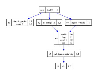
Figure 2: The graph of blocks of the method sum in Fig. 1, where each block is decorated with a unique name. On the right of each instruction, we report the number of local variables and stack elements at that program point, just before executing the instruction.

• The block $\mathit{sum}$ has $b_{1}$, $b_{2}$ and $b_{3}$ as successors and its first instruction is not a $\mathsf{call}$ instruction. Let $q$ be the program point where the instruction $\mathsf{load}\ 0$ of the block $\mathit{sum}$ occurs. We have

  $$\mathit{load}_{q}^{\mathbb{PL}}\ 0 =\mathit{Unchanged}_{q}(1,0)\cup\{\check{{l}}^{0}=\hat{{s}}^{0}\}$$

  $$=\{\check{{l}}^{0}=\hat{{l}}^{0},\check{{l}}^{0}=\hat{{s}}^{0}\}\;.$$

  Hence, by Definition 12, $\mathit{sum}_{\mathit{CLP}}$ consists of the following clauses:

  $$\mathit{sum}(\check{{l}}^{0},\check{{s}}_{\mathit{sum}})\mathop{\leftarrow}\limits\; \{\check{{l}}^{0}=\hat{{l}}^{0},\check{{l}}^{0}=\hat{{s}}^{0},\check{{s}}_{\mathit{sum}}=\hat{{s}}_{\mathit{sum}}\},$$

  $$b_{1}(\hat{{l}}^{0},\hat{{s}}^{0},\hat{{s}}_{\mathit{sum}})$$

  $$\mathit{sum}(\check{{l}}^{0},\check{{s}}_{\mathit{sum}})\mathop{\leftarrow}\limits\; \{\check{{l}}^{0}=\hat{{l}}^{0},\check{{l}}^{0}=\hat{{s}}^{0},\check{{s}}_{\mathit{sum}}=\hat{{s}}_{\mathit{sum}}\},$$

  $$b_{2}(\hat{{l}}^{0},\hat{{s}}^{0},\hat{{s}}_{\mathit{sum}})$$

  $$\mathit{sum}(\check{{l}}^{0},\check{{s}}_{\mathit{sum}})\mathop{\leftarrow}\limits\; \{\check{{l}}^{0}=\hat{{l}}^{0},\check{{l}}^{0}=\hat{{s}}^{0},\check{{s}}_{\mathit{sum}}=\hat{{s}}_{\mathit{sum}}\},$$

  $$b_{3}(\hat{{l}}^{0},\hat{{s}}^{0},\hat{{s}}_{\mathit{sum}})\;.$$

• The block $b_{1}$ has no successor and its first instruction is not a $\mathsf{call}$ instruction. Let $q$ and $q^{\prime}$ be the program points where the instructions $\mathsf{ifeq\ of\ type}\ \mathtt{int}$ and $\mathsf{const}\ 0$ of the block $b_{1}$ occur, respectively. We have

  $$\;(\mathit{ifeq\ of\ type}_{q}^{\mathbb{PL}}\ \mathtt{int});^{\mathbb{PL}}(\mathit{const}_{q^{\prime}}^{\mathbb{PL}}\ 0)$$

  $$= \;(\mathit{Unchanged}_{q}(1,0)\cup\{\check{{s}}^{0}=0\})$$

  $$\quad;^{\mathbb{PL}}(\mathit{Unchanged}_{q^{\prime}}(1,0)\cup\{0=\hat{{s}}^{0}\})$$

  $$= \;\{\check{{l}}^{0}=\hat{{l}}^{0},\check{{s}}^{0}=0\};^{\mathbb{PL}}\{\check{{l}}^{0}=\hat{{l}}^{0},0=\hat{{s}}^{0}\}$$

  $$= \;\{\check{{l}}^{0}=\hat{{l}}^{0},\check{{s}}^{0}=0,0=\hat{{s}}^{0}\}\;.$$

  Hence, by Definition 12, ${b_{1}}_{\mathit{CLP}}$ consists of the following clause:

  $$\begin{array}[]{l}b_{1}(\check{{l}}^{0},\check{{s}}^{0},\check{{s}}_{b_{1}})\mathop{\leftarrow}\limits\{\check{{l}}^{0}=\hat{{l}}^{0},\check{{s}}^{0}=0,0=\hat{{s}}^{0},\check{{s}}_{b_{1}}=\hat{{s}}^{0}\}\;.\end{array}$$

• The block $b_{5}$ consists of only one instruction, which is a call to a static method, and it has $b_{6}$ as unique successor. We have

  $$c_{=}=\{\check{{l}}^{0}=\hat{{l}}^{0},\check{{s}}^{0}=\hat{{s}}^{0}\}\;.$$

  Hence, by Definition 14, ${b_{5}}_{\mathit{CLP}}$ consists of the following clause:

  $$b_{5}(\check{{l}}^{0},\check{{s}}^{0},\check{{s}}^{1},\check{{s}}_{b_{5}})\mathop{\leftarrow}\limits\; \{\check{{l}}^{0}=\hat{{l}}^{0},\check{{s}}^{0}=\hat{{s}}^{0},\check{{s}}_{b_{5}}=\hat{{s}}_{b_{5}}\},$$

  $$\mathit{sum}(\check{{s}}^{1},\hat{{s}}^{1}),b_{6}(\hat{{l}}^{0},\hat{{s}}^{0},\hat{{s}}^{1},\hat{{s}}_{b_{5}})\;.$$

The complete $\mathrm{CLP}(\mathbb{PL})$ program derived from the program in Fig. 1 consists of the clauses in Table 1. ∎

$$\begin{array}[]{|cl|}\hline\cr\vrule\lx@intercol\hfil\texttt{sum}\hfil\lx@intercol\vrule\lx@intercol\\ \hline\cr(r_{1})&\mathit{sum}(\check{{l}}^{0},\check{{s}}_{\mathit{sum}})\mathop{\leftarrow}\limits\{\check{{l}}^{0}=\hat{{l}}^{0},\check{{l}}^{0}=\hat{{s}}^{0},\check{{s}}_{\mathit{sum}}=\hat{{s}}_{\mathit{sum}}\},\\ &\hskip 59.75095ptb_{1}(\hat{{l}}^{0},\hat{{s}}^{0},\hat{{s}}_{\mathit{sum}})\\[3.87498pt] (r_{2})&\mathit{sum}(\check{{l}}^{0},\check{{s}}_{\mathit{sum}})\mathop{\leftarrow}\limits\{\check{{l}}^{0}=\hat{{l}}^{0},\check{{l}}^{0}=\hat{{s}}^{0},\check{{s}}_{\mathit{sum}}=\hat{{s}}_{\mathit{sum}}\},\\ &\hskip 59.75095ptb_{2}(\hat{{l}}^{0},\hat{{s}}^{0},\hat{{s}}_{\mathit{sum}})\\[3.87498pt] (r_{3})&\mathit{sum}(\check{{l}}^{0},\check{{s}}_{\mathit{sum}})\mathop{\leftarrow}\limits\{\check{{l}}^{0}=\hat{{l}}^{0},\check{{l}}^{0}=\hat{{s}}^{0},\check{{s}}_{\mathit{sum}}=\hat{{s}}_{\mathit{sum}}\},\\ &\hskip 59.75095ptb_{3}(\hat{{l}}^{0},\hat{{s}}^{0},\hat{{s}}_{\mathit{sum}})\\[3.87498pt] (r_{4})&b_{1}(\check{{l}}^{0},\check{{s}}^{0},\check{{s}}_{b_{1}})\mathop{\leftarrow}\limits\{\check{{l}}^{0}=\hat{{l}}^{0},\check{{s}}^{0}=0,0=\hat{{s}}^{0},\check{{s}}_{b_{1}}=\hat{{s}}^{0}\}\\[3.87498pt] (r_{5})&b_{2}(\check{{l}}^{0},\check{{s}}^{0},\check{{s}}_{b_{2}})\mathop{\leftarrow}\limits\{\check{{l}}^{0}=\hat{{l}}^{0},\check{{s}}^{0}\leq-1,\check{{s}}_{b_{2}}=\hat{{s}}_{b_{2}}\},\\ &\hskip 56.9055ptb_{4}(\hat{{l}}^{0},\hat{{s}}_{b_{2}})\\[3.87498pt] (r_{6})&b_{3}(\check{{l}}^{0},\check{{s}}^{0},\check{{s}}_{b_{3}})\mathop{\leftarrow}\limits\{\check{{l}}^{0}=\hat{{l}}^{0},\check{{s}}^{0}\geq 1,\check{{s}}_{b_{3}}=\hat{{s}}_{b_{3}}\},\\ &\hskip 56.9055ptb_{4}(\hat{{l}}^{0},\hat{{s}}_{b_{3}})\\[3.87498pt] (r_{7})&b_{4}(\check{{l}}^{0},\check{{s}}_{b_{4}})\mathop{\leftarrow}\limits\{\check{{l}}^{0}=\hat{{l}}^{0},\check{{l}}^{0}=\hat{{s}}^{0},\check{{l}}^{0}-1=\hat{{s}}^{1},\check{{s}}_{b_{4}}=\hat{{s}}_{b_{4}}\},\\ &\hskip 45.52458ptb_{5}(\hat{{l}}^{0},\hat{{s}}^{0},\hat{{s}}^{1},\hat{{s}}_{b_{4}})\\[3.87498pt] (r_{8})&b_{5}(\check{{l}}^{0},\check{{s}}^{0},\check{{s}}^{1},\check{{s}}_{b_{5}})\mathop{\leftarrow}\limits\{\check{{l}}^{0}=\hat{{l}}^{0},\check{{s}}^{0}=\hat{{s}}^{0},\check{{s}}_{b_{5}}=\hat{{s}}_{b_{5}}\},\\ &\hskip 71.13188pt\mathit{sum}(\check{{s}}^{1},\hat{{s}}^{1}),b_{6}(\hat{{l}}^{0},\hat{{s}}^{0},\hat{{s}}^{1},\hat{{s}}_{b_{5}})\\[3.87498pt] (r_{9})&b_{6}(\check{{l}}^{0},\check{{s}}^{0},\check{{s}}^{1},\check{{s}}_{b_{6}})\mathop{\leftarrow}\limits\{\check{{l}}^{0}=\hat{{l}}^{0},\check{{s}}^{0}+\check{{s}}^{1}=\hat{{s}}^{0},\check{{s}}_{b_{6}}=\hat{{s}}^{0}\}\\ \hline\cr\hline\cr\vrule\lx@intercol\hfil\texttt{main}\hfil\lx@intercol\vrule\lx@intercol\\ \hline\cr(r_{10})&\mathit{main}(\check{{l}}^{0})\mathop{\leftarrow}\limits\{\check{{l}}^{0}=\hat{{l}}^{0},-1=\hat{{s}}^{0}\},b_{7}(\hat{{l}}^{0},\hat{{s}}^{0})\\[3.87498pt] (r_{11})&b_{7}(\check{{l}}^{0},\check{{s}}^{0})\mathop{\leftarrow}\limits\{\check{{l}}^{0}=\hat{{l}}^{0}\},\mathit{sum}(\check{{s}}^{0},\hat{{s}}^{0}),b_{8}(\hat{{l}}^{0},\hat{{s}}^{0})\\[3.87498pt] (r_{12})&b_{8}(\check{{l}}^{0},\check{{s}}^{0})\mathop{\leftarrow}\limits\{\check{{l}}^{0}=\hat{{l}}^{0}\}\\ \hline\cr\end{array}$$

Table 1: The $\mathrm{CLP}(\mathbb{PL})$ program derived from the program in Fig. 1

5 Proving Non-Termination

Let $P$ be a Java bytecode program and $b$ be a block of $P$. By Theorem 2, the existence of an infinite computation in $P_{\mathit{CLP}}$ of a query of the form $b(\cdots)$ entails that there is an execution of the Java Virtual Machine starting at $b$ that does not terminate. In [20], we provide a criterion that can be used for proving the existence of a non-terminating query for a binary $\mathrm{CLP}(\mathbb{PL})$ program i.e., a program consisting of clauses whose body contains at most one atom (we refer to such clauses as binary clauses). Note that by Definitions 13–14, $P_{\mathit{CLP}}$ may not be binary as it may contain clauses whose body consists of two atoms.

We use the binary unfolding operation [12] to transform $P_{\mathit{CLP}}$ into a binary program. We write $\mathrm{CLP}(\mathbb{PL})$ clauses as

$$H\mathop{\leftarrow}\limits c,B_{1},\ldots,B_{m}\quad\text{or}\quad H\mathop{\leftarrow}\limits c,\mathbf{B}$$

where $c$ is a $\mathrm{CLP}(\mathbb{PL})$ constraint, $H$, $B_{1}$, …, $B_{m}$ are atoms and $\mathbf{B}$ is a sequence of atoms. When $B_{1},\ldots,B_{m}$ or $\mathbf{B}$ are empty sequences, we write the clause as $H\mathop{\leftarrow}\limits c$. We let $\mathit{id}$ denote the set of all the binary clauses of the form

$$p(\tilde{x})\mathop{\leftarrow}\limits\{\tilde{x}=\tilde{y}\},p(\tilde{y})$$

where $p$ is a predicate symbol and $\tilde{x}$ and $\tilde{y}$ are disjoint sequences of distinct variables. We also let $\overline{\exists}_{\mathit{Var}(H,\mathbf{B})}[\cdots]$ denote the projection of $[\cdots]$ onto the variables of $H$ and $\mathbf{B}$.

Definition 16.

Let $P_{\mathit{CLP}}$ be a $\mathrm{CLP}(\mathbb{PL})$ program and $X$ be a set of binary clauses. Then,

$$T_{P_{\mathit{CLP}}}^{\beta}(X)=\mathcal{F}\cup\mathcal{B}$$

where

$$\mathcal{F}=\big{\{}H\mathop{\leftarrow}\limits c\in P_{\mathit{CLP}}\,|\,c\text{ is satisfiable}\big{\}}$$

and $\mathcal{B}$ is the set

$$\begin{array}[]{l}\left\{H\mathop{\leftarrow}\limits c,\mathbf{B}\begin{array}[]{@{\;}|@{\;}l}r=H\mathop{\leftarrow}\limits c_{0},B_{1},\ldots,B_{m}\in P_{\mathit{CLP}},\ 1\leq i\leq m\\[3.87498pt] \langle H_{j}\leftarrow c_{j}\rangle_{j=1}^{i-1}\in X\mbox{ renamed apart from $r$}\\[3.87498pt] H_{i}\leftarrow c_{i},\mathbf{B}\in X\cup\mathit{id}\mbox{ renamed apart from $r$}\\[3.87498pt] i<m\Rightarrow\mathbf{B}\neq\varnothing\\[3.87498pt] c=\overline{\exists}_{\mathit{Var}(H,\mathbf{B})}\big{[}c_{0}\land\mathop{\land}\limits_{j=1}^{i}(c_{j}\land B_{j}=H_{j})\big{]}\\[3.87498pt] c\mbox{ is satisfiable}\end{array}\right\}\end{array}$$

We define the powers of $T_{P_{\mathit{CLP}}}^{\beta}$ as usual:

$$T_{P_{\mathit{CLP}}}^{\beta}\uparrow 0 =\varnothing$$

$$T_{P_{\mathit{CLP}}}^{\beta}\uparrow(i+1) =T_{P_{\mathit{CLP}}}^{\beta}(T_{P_{\mathit{CLP}}}^{\beta}\uparrow i)\quad\forall i\in{\rm Nature}\;.$$

It can be shown that the least fixpoint ($\mathit{lfp}$) of this monotonic operator always exists and we set

$$\mathit{binunf}(P_{\mathit{CLP}})=\mathit{lfp}(T_{P_{\mathit{CLP}}}^{\beta})\;.$$

∎

Example 8.

Consider the program $P_{\mathit{CLP}}$ in Table 1.

We have $T_{P_{\mathit{CLP}}}^{\beta}\uparrow 0=\varnothing$. Moreover,

• the set $T_{P_{\mathit{CLP}}}^{\beta}\uparrow 1$ includes the following clauses:

  $$\begin{array}[]{cr@{\;\la\;}l}(u_{1})&b_{5}(\check{{l}}^{0},\check{{s}}^{0},\check{{s}}^{1},\check{{s}}_{b_{5}})\;\mathop{\leftarrow}\limits&\{\},\mathit{sum}(\check{{s}}^{1},\hat{{s}}^{1})\\[4.30554pt] (u_{2})&b_{7}(\check{{l}}^{0},\check{{s}}^{0})\;\mathop{\leftarrow}\limits&\{\},\mathit{sum}(\check{{s}}^{0},\hat{{s}}^{0})\end{array}$$

  where $u_{1}$ is obtained by unfolding $r_{8}$ with $\mathit{id}$ and $u_{2}$ by unfolding $r_{11}$ with $\mathit{id}$,

• the set $T_{P_{\mathit{CLP}}}^{\beta}\uparrow 2$ includes the following clauses:

  $$\begin{array}[]{cr@{\;\la\;}l}(u_{3})&b_{4}(\check{{l}}^{0},\check{{s}}_{b_{4}})\;\mathop{\leftarrow}\limits&\{\check{{l}}^{0}-1=\check{{s}}^{1}\},\mathit{sum}(\check{{s}}^{1},\hat{{s}}^{1})\\[4.30554pt] (u_{4})&\mathit{main}(\check{{l}}^{0})\;\mathop{\leftarrow}\limits&\{-1=\check{{s}}^{0}\},\mathit{sum}(\check{{s}}^{0},\hat{{s}}^{0})\end{array}$$

  where $u_{3}$ is obtained by unfolding $r_{7}$ with $u_{1}$ and $u_{4}$ by unfolding $r_{10}$ with $u_{2}$,

• the set $T_{P_{\mathit{CLP}}}^{\beta}\uparrow 3$ includes the following clause, obtained by unfolding $r_{5}$ with $u_{3}$:

  $$(u_{5})\quad b_{2}(\check{{l}}^{0},\check{{s}}^{0},\check{{s}}_{b_{2}})\mathop{\leftarrow}\limits\; \{\check{{l}}^{0}-1=\check{{s}}^{1},\check{{s}}^{0}\leq-1\},$$

  $$\mathit{sum}(\check{{s}}^{1},\hat{{s}}^{1})$$

• the set $T_{P_{\mathit{CLP}}}^{\beta}\uparrow 4$ includes the following clause, obtained by unfolding $r_{2}$ with $u_{5}$:

  $$(u_{6})\quad\mathit{sum}(\check{{l}}^{0},\check{{s}}_{\mathit{sum}})\mathop{\leftarrow}\limits\; \{\check{{l}}^{0}\leq-1,\check{{l}}^{0}-1=\check{{s}}^{1}\},$$

  $$\mathit{sum}(\check{{s}}^{1},\hat{{s}}^{1})\;.$$

  ∎

It is proved in [9] that existential non-termination in $P_{\mathit{CLP}}$ is equivalent to existential non-termination in $\mathit{binunf}(P_{\mathit{CLP}})$:

Theorem 3

Let $P_{\mathit{CLP}}$ be a $\mathrm{CLP}(\mathbb{PL})$ program and $Q$ be a query consisting of one atom. Then, $Q$ has an infinite computation in $P_{\mathit{CLP}}$ if and only if $Q$ has an infinite computation in $\mathit{binunf}(P_{\mathit{CLP}})$.

Note that $\mathit{binunf}(P_{\mathit{CLP}})$ is a possibly infinite set of binary clauses. In practice, we compute only the first $\mathit{max}$ iterations of $T_{P_{\mathit{CLP}}}^{\beta}$, where $\mathit{max}$ is a parameter of the analysis, and we have $T_{P_{\mathit{CLP}}}^{\beta}\uparrow\mathit{max}\subseteq\mathit{binunf}(P_{\mathit{CLP}})$. Therefore, any query that has an infinite computation in $T_{P_{\mathit{CLP}}}^{\beta}\uparrow\mathit{max}$ also has an infinite computation in $\mathit{binunf}(P_{\mathit{CLP}})$, hence, by Theorem 3, in $P_{\mathit{CLP}}$.

In the results we present below, $p$ is a predicate symbol, $\tilde{x}$ and $\tilde{y}$ are disjoint sequences of distinct variables and $c$ is a $\mathrm{CLP}(\mathbb{PL})$ constraint on $\tilde{x}$ and $\tilde{y}$ only (i.e., the set of variables appearing in $c$ is a subset of $\tilde{x}\cup\tilde{y}$). The criterion that we provide in [20] for proving the existence of a non-terminating query can be formulated as follows in the context of $\mathrm{CLP}(\mathbb{PL})$ clauses.

Proposition 3

Let

$$r=p(\tilde{x})\mathop{\leftarrow}\limits c,p(\tilde{y})$$

be a $\mathrm{CLP}(\mathbb{PL})$ binary clause where $c$ is satisfiable. Let $e(\tilde{x})$ denote the projection of $c$ onto $\tilde{x}$. Suppose the formula

$$\forall\tilde{x}\ e(\tilde{x})\Rightarrow\big{[}\forall\tilde{y}\ c\Rightarrow e(\tilde{y})\big{]}$$

is true. Then, $p(\tilde{v})$ has an infinite computation in $\{r\}$, for some fixed integer values for $\tilde{v}$.

The sense of Proposition 3 is the following. Satisfiability for $c$ means that there exists some “input” to the clause i.e., some value from which one can “enter” the clause. The logical formula means: let $\tilde{a}$ be some input to the clause (i.e., $\forall\tilde{x}\ e(\tilde{x})$), then any output $\tilde{b}$ corresponding to $\tilde{a}$ (i.e., $\forall\tilde{y}\ c$) is also an input to the clause (i.e., $e(\tilde{y})$). Shortly, if one can enter the clause with $\tilde{a}$, then one can enter the clause again with any output corresponding to $\tilde{a}$. This corresponds to a notion of unavoidable (universal) non-termination, as any input to the clause necessarily leads to an infinite computation.

The criterion provided in Proposition 3 can be refined into:

Proposition 4

Let

$$r=p(\tilde{x})\mathop{\leftarrow}\limits c,p(\tilde{y})$$

be a $\mathrm{CLP}(\mathbb{PL})$ binary clause where $c$ is satisfiable. Let $e(\tilde{x})$ denote the projection of $c$ onto $\tilde{x}$. Suppose the formula

$$\forall\tilde{x}\ e(\tilde{x})\Rightarrow\big{[}\exists\tilde{y}\ c\land e(\tilde{y})\big{]}$$

is true. Then, $p(\tilde{v})$ has an infinite computation in $\{r\}$, for some fixed integer values for $\tilde{v}$.

Now, the sense of the logical formula is: if one can enter the clause with an input $\tilde{a}$, then there exists an output $\tilde{b}$ corresponding to $\tilde{a}$ such that one can enter the clause again with $\tilde{b}$. This corresponds to a notion of potential (existential) non-termination, as for any input to the clause there is a corresponding output that leads to an infinite computation.

The criterion of Proposition 3 entails that of Proposition 4, but the converse does not hold in general (e.g., for the clause $p(x)\mathop{\leftarrow}\limits\{x\geq 0\},p(y)$ the logical formula of Proposition 4 is true whereas that of Proposition 3 is not).

In Proposition 4, we consider recursive binary clauses. A recursive clause in $\mathit{binunf}(P_{\mathit{CLP}})$ is a compressed form of a loop in $P_{\mathit{CLP}}$. The next result allows one to ensure that a loop is reachable from a given program point.

Proposition 5

Let

$$\begin{array}[]{r@{\;=\;}l}r&p(\tilde{x})\mathop{\leftarrow}\limits c,p(\tilde{y})\\[6.45831pt] r^{\prime}&p^{\prime}(\tilde{x}^{\prime})\mathop{\leftarrow}\limits c^{\prime},p(\tilde{y}^{\prime})\end{array}$$

be some $\mathrm{CLP}(\mathbb{PL})$ binary clauses where $c$ and $c^{\prime}$ are satisfiable. Let $e(\tilde{x})$ denote the projection of $c$ onto $\tilde{x}$. Suppose the formulæ

• $\forall\tilde{x}\ e(\tilde{x})\Rightarrow\big{[}\exists\tilde{y}\ c\land e(\tilde{y})\big{]}$

• $\exists\tilde{x}^{\prime},\ \exists\tilde{y}^{\prime},\ c^{\prime}\land e(\tilde{y}^{\prime})$

are true. Then, $p^{\prime}(\tilde{v})$ has an infinite computation in $\{r,r^{\prime}\}$, for some fixed integer values for $\tilde{v}$.

The sense of the second logical formula in Proposition 5 is that there is an output to the clause $r^{\prime}$ which is an input to the clause $r$. Moreover, any input to $r^{\prime}$ that satisfies the second formula is the starting point of a potential infinite computation; if the first logical formula in Proposition 5 was that of Proposition 3, then it would be the starting point of an unavoidable infinite computation.

Example 9.

The clauses $u_{4}$ and $u_{6}$ in Example 8 satisfy the pre-conditions of Proposition 5. Hence, by Proposition 5, there is a value $v$ in $\mathbb{Z}$ which is such that $\mathit{main}(v)$ has an infinite computation in $\mathit{binunf}(P_{\mathit{CLP}})$, hence an infinite computation in $P_{\mathit{CLP}}$. Consequently, by Theorem 2, there is an execution of the Java virtual Machine started at block $\mathit{main}$ that does not terminate, where $\mathit{main}$ is the initial block of the Java bytecode program corresponding to the Java program in Fig. 1. ∎

6 Experiments

We implemented our approach in the Julia analyser. Non-termination proofs of $\mathrm{CLP}(\mathbb{PL})$ programs are performed by the BinTerm tool, a component of Julia that implements Proposition 5. BinTerm is written in SWI-Prolog [33] and relies on the Parma Polyhedra Library [3] for checking satisfiability of integer linear constraints. Elimination of existentially quantified variables in $\mathbb{Z}$ follows the approach of the Omega Test [25].

We evaluated our analyser on a collection of 113 examples, made up of:

• a set of 75 iterative examples, consisting of 54 programs provided by [16, 30] and the 21 non-terminating programs submitted by the Julia team to the International Termination Competition [29] in 2011,

• a set of 38 recursive examples, consisting of 34 programs that we obtained by turning some examples from [16, 30] into recursive programs, and 4 programs that we wrote ourselves; all of these recursive programs do not terminate due to an infinite recursion.

In our experiments, we compared AProVE, Invel and the new version of Julia. We used the default settings for each tool i.e., a time-out of 60 seconds for AProVE, a maximum number of iterations set to 10 for Invel and, for Julia, a time-out of 20 seconds for each strongly connected component of the $\mathrm{CLP}(\mathbb{PL})$ program. Details on the experiments are available at [24]. We do not provide running times as we could not run all the tools on a same machine (the AProVE implementation that performs non-termination proofs is available through a web interface only).

Table 2 and Table 3 give an overview of the results that we obtained. Here, “Invel” is the set of 54 examples from [16, 30], “Julia TC11” is the set of 21 non-terminating examples submitted by Julia to the competition in 2011, “Invel rec.” is the set obtained by turning 34 Invel examples into recursive programs and “Julia rec.” corresponds to the 4 programs that we wrote. Moreover, Y and N indicate how often termination (resp. non-termination) could be proved, F indicates how often a tool failed within the time limit set by its default settings and T states how many examples led to time-out. Finally, P (Problems) gives the number of times a tool stopped with a run-time exception or produced an incorrect answer: the Invel analyser issued 2 incorrect answers (2 terminating programs incorrectly proved non-terminating) and stopped twice with a NullPointerException. Table 2 shows that Julia failed on 22 Invel examples; 13 of these failures are due to the use, in the corresponding programs, of bytecode instructions that are not exactly abstracted into constraints. Table 3 clearly shows that only Julia could detect non-terminating recursions.

	Invel (54)					Julia TC11 (21)
	Y	N	F	T	P	N	F	T	P
AProVE	3	49	0	2	0	21	0	0	0
Invel	0	29	1	21	3	13	0	7	1
Julia	2	30	22	0	0	17	4	0	0

Table 2: The results of our experiments on iterative programs.

	Invel rec. (34)			Julia rec. (4)
	N	F	T	N	T
AProVE	0	0	34	0	4
Invel	0	0	34	0	4
Julia	26	8	0	4	0

Table 3: The results of our experiments on recursive programs.

Interpreting the Web Interface of Julia

For our experiments, there are three cases. Let us consider the Invel examples.

• For alternatingIncr.jar, we get one warning:

  [Termination] are you sure that
  simple.alternatingIncr.increase always
  terminates?
  

  It means that Julia has a proof that the upper approximation of the program built to prove termination loops in $\mathbb{Q}$, indicating a potential non-termination of the original program.

• For alternDiv.jar, we get two warnings:

  [Termination] are you sure that
  simple.alternDiv.AlternDiv.loop always
  terminates?
  
  [Termination] simple.alternDiv.Main.main may
  actually diverge
  

  The first warning has the same interpretation as above while the second one emphasizes that Julia has a non-termination proof for the original program.

• For whileBreak.jar, there are no warnings. It means that Julia has a termination proof for the original program.

7 Conclusion

The work we have presented in this paper was initiated in [22], where we observed that in some situations the non-termination of a Java bytecode program can be deduced from that of its $\mathrm{CLP}(\mathbb{PL})$ translation. Here, we have introduced the formal material that is missing in [22] and we have presented a new experimental evaluation, conducted with the Julia tool which now includes an implementation of our results. Currently, our non-termination analysis cannot be applied to programs that include certain types of object field access. We are actively working at extending its scope, so that it can identify sources of non-termination such as traversal of cyclical data structures.

Appendix A Proofs

A.1 Proposition 1

Let $\delta_{1}\in\Delta_{l_{i},s_{i}\to l_{t},s_{t}}$, $\delta_{2}\in\Delta_{l_{t},s_{t}\to l_{o},s_{o}}$, $\mathit{\mathit{pl}}_{1}\in\mathbb{PL}_{l_{i},s_{i}\to l_{t},s_{t}}$ and $\mathit{\mathit{pl}}_{2}\in\mathbb{PL}_{l_{t},s_{t}\to l_{o},s_{o}}$. Suppose that $\mathit{\mathit{pl}}_{1}\models\delta_{1}$, that $\mathit{\mathit{pl}}_{2}\models\delta_{2}$ and that $\delta_{1}$ is compatible with $\delta_{2}$. For sake of readability, we let $\mathit{\mathit{pl}}_{1,2}$ denote the constraint $\mathit{\mathit{pl}}_{1};^{\mathbb{PL}}\mathit{\mathit{pl}}_{2}$. We have $\delta_{1};\delta_{2}\in\Delta_{l_{i},s_{i}\to l_{o},s_{o}}$ and $\mathit{\mathit{pl}}_{1,2}\in\mathbb{PL}_{l_{i},s_{i}\to l_{o},s_{o}}$. We have to prove that $\mathit{\mathit{pl}}_{1,2}\models\delta_{1};\delta_{2}$. So, consider any model $\rho$ of $\mathit{\mathit{pl}}_{1,2}$ and any state $\sigma$ compatible with $\delta_{1};\delta_{2}$. Suppose that $\check{{len}}(\sigma)=\check{{\rho}}$. We have to prove that $(\delta_{1};\delta_{2})(\sigma)$ is defined and $\hat{{len}}((\delta_{1};\delta_{2})(\sigma))=\hat{{\rho}}$.

Let

$$T=\{\overline{l}^{0},\ldots,\overline{l}^{l_{t}-1},\overline{s}^{0},\ldots,\overline{s}^{s_{t}-1}\}\;.$$

By Definition 6,

$$\mathit{\mathit{pl}}_{1,2}=\exists_{T}\big{(}\mathit{\mathit{pl}}_{1}[\hat{{v}}\mapsto\overline{v}\;|\;\overline{v}\in T]\cup\mathit{\mathit{pl}}_{2}[\check{{v}}\mapsto\overline{v}\;|\;\overline{v}\in T]\big{)}\;.$$

As $\rho$ is a model of $\mathit{\mathit{pl}}_{1,2}$, there exists an assignment $\rho^{\prime}$ that coincides with $\rho$ on every variable not in $T$ and which is such that

$$\rho^{\prime}\models\mathit{\mathit{pl}}_{1}[\hat{{v}}\mapsto\overline{v}\;|\;\overline{v}\in T]\quad\text{and}\quad\rho^{\prime}\models\mathit{\mathit{pl}}_{2}[\check{{v}}\mapsto\overline{v}\;|\;\overline{v}\in T]\;.$$ (1)

Consider the following facts and definitions.

• The state $\sigma$ is compatible with $\delta_{1};\delta_{2}$, hence it is compatible with $\delta_{1}$.

• We define the assignment $\rho_{1}$ as:

  $$\begin{array}[]{rcl}\rho_{1}&=&[\check{{l}}^{k}\mapsto\rho^{\prime}(\check{{l}}^{k})\;|\;0\leq k<l_{i}]\\[4.30554pt] &\cup&[\check{{s}}^{k}\mapsto\rho^{\prime}(\check{{s}}^{k})\;|\;0\leq k<s_{i}]\\[4.30554pt] &\cup&[\hat{{v}}\mapsto\rho^{\prime}(\overline{v})\;|\;\overline{v}\in T]\;.\end{array}$$

  By (1), $\rho_{1}\models\mathit{\mathit{pl}}_{1}$, hence $\rho_{1}$ is a model of $\mathit{\mathit{pl}}_{1}$. Moreover, $\sigma$ is compatible with $\delta_{1}$ and $\check{{len}}(\sigma)=\check{{\rho}}$ with $\check{{\rho}}=\check{{\rho}}_{1}$. As $\mathit{\mathit{pl}}_{1}\models\delta_{1}$, then $\delta_{1}(\sigma)$ is defined and $\hat{{len}}(\delta_{1}(\sigma))=\hat{{\rho}}_{1}$.

• We define the assignment $\rho_{2}$ as:

  $$\begin{array}[]{rcl}\rho_{2}&=&[\check{{v}}\mapsto\rho^{\prime}(\overline{v})\;|\;\overline{v}\in T]\\[4.30554pt] &\cup&[\hat{{l}}^{k}\mapsto\rho^{\prime}(\hat{{l}}^{k})\;|\;0\leq k<l_{o}]\\[4.30554pt] &\cup&[\hat{{s}}^{k}\mapsto\rho^{\prime}(\hat{{s}}^{k})\;|\;0\leq k<s_{o}]\;.\end{array}$$

  By (1), $\rho_{2}\models\mathit{\mathit{pl}}_{2}$, hence $\rho_{2}$ is a model of $\mathit{\mathit{pl}}_{2}$. Moreover, $\delta_{1}(\sigma)$ is compatible with $\delta_{2}$ (because $\delta_{1}$ is compatible with $\delta_{2}$) and $\hat{{len}}(\delta_{1}(\sigma))=\hat{{\rho}}_{1}$. By definition of $\rho_{1}$ and $\rho_{2}$, for each variable $\overline{v}$ in $T$ we have $\rho_{1}(\hat{{v}})=\rho_{2}(\check{{v}})$. Hence, $\hat{{len}}(\delta_{1}(\sigma))=\hat{{\rho}}_{1}$ implies that $\check{{len}}(\delta_{1}(\sigma))=\check{{\rho}}_{2}$. As $\mathit{\mathit{pl}}_{2}\models\delta_{2}$, then $\delta_{2}(\delta_{1}(\sigma))$ is defined and we have $\hat{{len}}(\delta_{2}(\delta_{1}(\sigma)))=\hat{{\rho}}_{2}$ with $\hat{{\rho}}_{2}=\hat{{\rho}}$.

Consequently, $(\delta_{1};\delta_{2})(\sigma)$ is defined and $\hat{{len}}((\delta_{1};\delta_{2})(\sigma))=\hat{{\rho}}$.

A.2 Proposition 2

Let $q$ be a program point and $\#l,\#s$ be the number of local variables and stack elements at $q$. For any $L,S\subseteq{\rm Nature}$, we let

$$\mathit{Unchanged_{q}(L,S)} =\{\check{{l}}^{i}=\hat{{l}}^{i}\mid i\in L\}$$

$$\cup\{\check{{s}}^{i}=\hat{{s}}^{i}\mid i\in S\}$$

$$\cup\{\check{{s}}^{i}=\check{{s}}^{j}\mid 0\leq i,\ j<\#s,$$

$$\hskip 56.9055pts^{i}\text{ is an alias of }s^{j}\text{ at }q\}$$

$$\cup\{\check{{s}}^{i}=\check{{l}}^{j}\mid 0\leq i<\#s,\ 0\leq j<\#l,$$

$$\hskip 56.9055pts^{i}\text{ is an alias of }l^{j}\text{ at }q\}$$

$$\cup\{\check{{l}}^{i}=\check{{l}}^{j}\mid 0\leq i,\ j<\#l,$$

$$\hskip 56.9055ptl^{i}\text{ is an alias of }l^{j}\text{ at }q\}$$

$$\cup\{\check{{s}}^{i}\geq 0\mid 0\leq i<\#s,$$

$$\hskip 14.22636pt\text{$s^{i}$ does not have integer type at }q\}$$

$$\cup\{\check{{l}}^{i}\geq 0\mid 0\leq i<\#l,$$

$$\hskip 14.22636pt\text{$l^{i}$ does not have integer type at }q\}~{}.$$

For any $l,s\in{\rm Nature}$, we let

$$\mathit{Unchanged}_{q}(l,s)=\mathit{Unchanged}_{q}( \{0,\ldots,l-1\},$$

$$\{0,\ldots,s-1\}).$$

Let $\mathsf{ins}$ be an instruction in $\mathcal{C}\setminus\{\mathsf{call}\}$. We have to prove that $\mathit{ins}_{q}^{\mathbb{PL}}\models\mathit{ins}_{q}$. Hence, consider any model $\rho$ of $\mathit{ins}_{q}^{\mathbb{PL}}$ and any state $\sigma$ compatible with $\mathit{ins}_{q}$, and suppose that $\check{{\mathit{len}}}(\sigma)=\check{{\rho}}$. We have to prove that $\mathit{ins}_{q}(\sigma)$ is defined and that $\hat{{\mathit{len}}}(\mathit{ins}_{q}(\sigma))=\hat{{\rho}}$.

• Suppose that $\mathsf{ins}=\mathsf{const}\ c$. Then,

  $$\mathit{ins}_{q}^{\mathbb{PL}} =\begin{cases}\mathit{Unchanged}_{q}(\#l,\#s)\cup\{c=\hat{{s}}^{\#s}\}&\text{if $c\in\mathbb{Z}$}\\ \mathit{Unchanged}_{q}(\#l,\#s)\cup\{0=\hat{{s}}^{\#s}\}&\text{if $c=\mathtt{null}$}\end{cases}$$

  $$\mathit{ins}_{q} =\lambda\langle l\operatorname{\mid\!\mid}s\operatorname{\mid\!\mid}\mu\rangle.\langle l\operatorname{\mid\!\mid}c::s\operatorname{\mid\!\mid}\mu\rangle\;.$$

  Note that $\mathit{ins}_{q}(\sigma)$ is defined because $\mathit{ins}_{q}$ is defined for any state that is compatible with it. Without loss of generality, suppose that $\sigma$ has the form $\langle l\operatorname{\mid\!\mid}s\operatorname{\mid\!\mid}\mu\rangle$.

  • Let $j\in\{0,\ldots,\#l-1\}$ and $k\in\{0,\ldots,\#s-1\}$. By definition of $\mathit{ins}_{q}$, we have $\hat{{\mathit{len}}}(\mathit{ins}_{q}(\sigma))(\hat{{l}}^{j})=\check{{\mathit{len}}}(\sigma)(\check{{l}}^{j})$ and $\hat{{\mathit{len}}}(\mathit{ins}_{q}(\sigma))(\hat{{s}}^{k})=\check{{\mathit{len}}}(\sigma)(\check{{s}}^{k})$; as $\check{{\mathit{len}}}(\sigma)=\check{{\rho}}$, we have $\check{{\mathit{len}}}(\sigma)(\check{{l}}^{j})=\check{{\rho}}(\check{{l}}^{j})$ and we have $\check{{\mathit{len}}}(\sigma)(\check{{s}}^{k})=\check{{\rho}}(\check{{s}}^{k})$; moreover, as $\rho$ is a model of $\mathit{ins}_{q}^{\mathbb{PL}}$, with $\mathit{Unchanged}_{q}(\#l,\#s)\subseteq\mathit{ins}_{q}^{\mathbb{PL}}$, we have $\check{{\rho}}(\check{{l}}^{j})=\hat{{\rho}}(\hat{{l}}^{j})$ and $\check{{\rho}}(\check{{s}}^{k})=\hat{{\rho}}(\hat{{s}}^{k})$. Therefore,

    $$\hat{{\mathit{len}}}(\mathit{ins}_{q}(\sigma))(\hat{{l}}^{j})=\hat{{\rho}}(\hat{{l}}^{j})$$

    and

    $$\hat{{\mathit{len}}}(\mathit{ins}_{q}(\sigma))(\hat{{s}}^{k})=\hat{{\rho}}(\hat{{s}}^{k})\;.$$

  • Suppose that $c\in\mathbb{Z}$. By definition of $\mathit{ins}_{q}$, we have $\hat{{\mathit{len}}}(\mathit{ins}_{q}(\sigma))(\hat{{s}}^{\#s})=\mathit{len}(c,\mu)=c$. As $\rho$ is a model of $\mathit{ins}_{q}^{\mathbb{PL}}$, with $\{c=\hat{{s}}^{\#s}\}\subseteq\mathit{ins}_{q}^{\mathbb{PL}}$, we have $\hat{{\rho}}(\hat{{s}}^{\#s})=c$. Hence,

    $$\hat{{\mathit{len}}}(\mathit{ins}_{q}(\sigma))(\hat{{s}}^{\#s})=\hat{{\rho}}(\hat{{s}}^{\#s})\;.$$

  • Suppose that $c=\mathtt{null}$. By definition of $\mathit{ins}_{q}$, $\hat{{\mathit{len}}}(\mathit{ins}_{q}(\sigma))(\hat{{s}}^{\#s})=\mathit{len}(c,\mu)=\mathit{len}(\mathtt{null},\mu)=0$. As $\rho$ is a model of $\mathit{ins}_{q}^{\mathbb{PL}}$, with $\{0=\hat{{s}}^{\#s}\}\subseteq\mathit{ins}_{q}^{\mathbb{PL}}$, we have $\hat{{\rho}}(\hat{{s}}^{\#s})=0$. Hence,

    $$\hat{{\mathit{len}}}(\mathit{ins}_{q}(\sigma))(\hat{{s}}^{\#s})=\hat{{\rho}}(\hat{{s}}^{\#s})\;.$$

  Consequently, we have $\hat{{\mathit{len}}}(\mathit{ins}_{q}(\sigma))=\hat{{\rho}}$.

• Suppose that $\mathsf{ins}=\mathsf{dup}$. Then,

  $$\mathit{ins}_{q}^{\mathbb{PL}} =\mathit{Unchanged}_{q}(\#l,\#s)\cup\{\check{{s}}^{\#s-1}=\hat{{s}}^{\#s}\}$$

  $$\mathit{ins}_{q} =\lambda\langle l\operatorname{\mid\!\mid}\mathit{top}::s\operatorname{\mid\!\mid}\mu\rangle.\langle l\operatorname{\mid\!\mid}\mathit{top}::\mathit{top}::s\operatorname{\mid\!\mid}\mu\rangle\;.$$

  Note that $\#s\geq 1$ and that $\mathit{ins}_{q}(\sigma)$ is defined because $\mathit{ins}_{q}$ is defined for any state that is compatible with it. Without loss of generality, suppose that $\sigma$ has the form $\langle l\operatorname{\mid\!\mid}\mathit{top}::s\operatorname{\mid\!\mid}\mu\rangle$.

  • Let $j\in\{0,\ldots,\#l-1\}$ and $k\in\{0,\ldots,\#s-1\}$. By definition of $\mathit{ins}_{q}$, we have $\hat{{\mathit{len}}}(\mathit{ins}_{q}(\sigma))(\hat{{l}}^{j})=\check{{\mathit{len}}}(\sigma)(\check{{l}}^{j})$ and $\hat{{\mathit{len}}}(\mathit{ins}_{q}(\sigma))(\hat{{s}}^{k})=\check{{\mathit{len}}}(\sigma)(\check{{s}}^{k})$; as $\check{{\mathit{len}}}(\sigma)=\check{{\rho}}$, we have $\check{{\mathit{len}}}(\sigma)(\check{{l}}^{j})=\check{{\rho}}(\check{{l}}^{j})$ and we have $\check{{\mathit{len}}}(\sigma)(\check{{s}}^{k})=\check{{\rho}}(\check{{s}}^{k})$; moreover, as $\rho$ is a model of $\mathit{ins}_{q}^{\mathbb{PL}}$, with $\mathit{Unchanged}_{q}(\#l,\#s)\subseteq\mathit{ins}_{q}^{\mathbb{PL}}$, we have $\check{{\rho}}(\check{{l}}^{j})=\hat{{\rho}}(\hat{{l}}^{j})$ and $\check{{\rho}}(\check{{s}}^{k})=\hat{{\rho}}(\hat{{s}}^{k})$. Therefore,

    $$\hat{{\mathit{len}}}(\mathit{ins}_{q}(\sigma))(\hat{{l}}^{j})=\hat{{\rho}}(\hat{{l}}^{j})$$

    and

    $$\hat{{\mathit{len}}}(\mathit{ins}_{q}(\sigma))(\hat{{s}}^{k})=\hat{{\rho}}(\hat{{s}}^{k})\;.$$

  • By definition of $\mathit{ins}_{q}$, we have $\hat{{\mathit{len}}}(\mathit{ins}_{q}(\sigma))(\hat{{s}}^{\#s})=\mathit{len}(\mathit{top},\mu)$ with $\mathit{len}(\mathit{top},\mu)=\check{{\mathit{len}}}(\sigma)(\check{{s}}^{\#s-1})$. As $\check{{\mathit{len}}}(\sigma)=\check{{\rho}}$, we have $\check{{\mathit{len}}}(\sigma)(\check{{s}}^{\#s-1})=\check{{\rho}}(\check{{s}}^{\#s-1})$. As $\rho$ is a model of $\mathit{ins}_{q}^{\mathbb{PL}}$, with $\{\check{{s}}^{\#s-1}=\hat{{s}}^{\#s}\}\subseteq\mathit{ins}_{q}^{\mathbb{PL}}$, we have $\check{{\rho}}(\check{{s}}^{\#s-1})=\hat{{\rho}}(\hat{{s}}^{\#s})$. Hence,

    $$\hat{{\mathit{len}}}(\mathit{ins}_{q}(\sigma))(\hat{{s}}^{\#s})=\hat{{\rho}}(\hat{{s}}^{\#s})\;.$$

  Consequently, we have $\hat{{\mathit{len}}}(\mathit{ins}_{q}(\sigma))=\hat{{\rho}}$.

• Suppose that $\mathsf{ins}=\mathsf{new}\ \kappa$. Then,

  $$\mathit{ins}_{q}^{\mathbb{PL}} =\mathit{Unchanged}_{q}(\#l,\#s)\cup\{1=\hat{{s}}^{\#s}\}$$

  $$\mathit{ins_{q}} =\lambda\langle l\operatorname{\mid\!\mid}s\operatorname{\mid\!\mid}\mu\rangle.\langle l\operatorname{\mid\!\mid}\ell::s\operatorname{\mid\!\mid}\mu[\ell\mapsto o]\rangle$$

  where $$\ell$$ is a fresh location

  and $$o \kappa$$ is an object of class

  whose fields hold $0$ or $\mathtt{null}$.

  Note that $\mathit{ins}_{q}(\sigma)$ is defined because we assume that $\mathit{ins}_{q}$ is a total map defined for any state that is compatible with it. Without loss of generality, suppose that $\sigma$ has the form $\langle l\operatorname{\mid\!\mid}s\operatorname{\mid\!\mid}\mu\rangle$.

  • Let $j\in\{0,\ldots,\#l-1\}$ and $k\in\{0,\ldots,\#s-1\}$. By definition of $\mathit{ins}_{q}$, we have $\hat{{\mathit{len}}}(\mathit{ins}_{q}(\sigma))(\hat{{l}}^{j})=\check{{\mathit{len}}}(\sigma)(\check{{l}}^{j})$ and $\hat{{\mathit{len}}}(\mathit{ins}_{q}(\sigma))(\hat{{s}}^{k})=\check{{\mathit{len}}}(\sigma)(\check{{s}}^{k})$; as $\check{{\mathit{len}}}(\sigma)=\check{{\rho}}$, we have $\check{{\mathit{len}}}(\sigma)(\check{{l}}^{j})=\check{{\rho}}(\check{{l}}^{j})$ and we have $\check{{\mathit{len}}}(\sigma)(\check{{s}}^{k})=\check{{\rho}}(\check{{s}}^{k})$; moreover, as $\rho$ is a model of $\mathit{ins}_{q}^{\mathbb{PL}}$, with $\mathit{Unchanged}_{q}(\#l,\#s)\subseteq\mathit{ins}_{q}^{\mathbb{PL}}$, we have $\check{{\rho}}(\check{{l}}^{j})=\hat{{\rho}}(\hat{{l}}^{j})$ and $\check{{\rho}}(\check{{s}}^{k})=\hat{{\rho}}(\hat{{s}}^{k})$. Therefore,

    $$\hat{{\mathit{len}}}(\mathit{ins}_{q}(\sigma))(\hat{{l}}^{j})=\hat{{\rho}}(\hat{{l}}^{j})$$

    and

    $$\hat{{\mathit{len}}}(\mathit{ins}_{q}(\sigma))(\hat{{s}}^{k})=\hat{{\rho}}(\hat{{s}}^{k})\;.$$

  • By definition of $\mathit{ins}_{q}$, we have $\hat{{\mathit{len}}}(\mathit{ins}_{q}(\sigma))(\hat{{s}}^{\#s})=\mathit{len}(\ell,\mu)=1$. As $\rho$ is a model of $\mathit{ins}_{q}^{\mathbb{PL}}$, with $\{1=\hat{{s}}^{\#s}\}\subseteq\mathit{ins}_{q}^{\mathbb{PL}}$, we have $1=\hat{{\rho}}(\hat{{s}}^{\#s})$. Hence,

    $$\hat{{\mathit{len}}}(\mathit{ins}_{q}(\sigma))(\hat{{s}}^{\#s})=\hat{{\rho}}(\hat{{s}}^{\#s})\;.$$

  Consequently, we have $\hat{{\mathit{len}}}(\mathit{ins}_{q}(\sigma))=\hat{{\rho}}$.

• Suppose that $\mathsf{ins}=\mathsf{load}\ i$. Then,

  $$\mathit{ins}_{q}^{\mathbb{PL}} =\mathit{Unchanged}_{q}(\#l,\#s)\cup\{\check{{l}}^{i}=\hat{{s}}^{\#s}\}$$

  $$\mathit{ins}_{q} =\lambda\langle l\operatorname{\mid\!\mid}s\operatorname{\mid\!\mid}\mu\rangle.\langle l\operatorname{\mid\!\mid}l^{i}::s\operatorname{\mid\!\mid}\mu\rangle\;.$$

  Note that $\mathit{ins}_{q}(\sigma)$ is defined because $\mathit{ins}_{q}$ is defined for any state that is compatible with it. Without loss of generality, suppose that $\sigma$ has the form $\langle l\operatorname{\mid\!\mid}s\operatorname{\mid\!\mid}\mu\rangle$.

  • Let $j\in\{0,\ldots,\#l-1\}$ and $k\in\{0,\ldots,\#s-1\}$. By definition of $\mathit{ins}_{q}$, we have $\hat{{\mathit{len}}}(\mathit{ins}_{q}(\sigma))(\hat{{l}}^{j})=\check{{\mathit{len}}}(\sigma)(\check{{l}}^{j})$ and $\hat{{\mathit{len}}}(\mathit{ins}_{q}(\sigma))(\hat{{s}}^{k})=\check{{\mathit{len}}}(\sigma)(\check{{s}}^{k})$; as $\check{{\mathit{len}}}(\sigma)=\check{{\rho}}$, we have $\check{{\mathit{len}}}(\sigma)(\check{{l}}^{j})=\check{{\rho}}(\check{{l}}^{j})$ and we have $\check{{\mathit{len}}}(\sigma)(\check{{s}}^{k})=\check{{\rho}}(\check{{s}}^{k})$; moreover, as $\rho$ is a model of $\mathit{ins}_{q}^{\mathbb{PL}}$, with $\mathit{Unchanged}_{q}(\#l,\#s)\subseteq\mathit{ins}_{q}^{\mathbb{PL}}$, we have $\check{{\rho}}(\check{{l}}^{j})=\hat{{\rho}}(\hat{{l}}^{j})$ and $\check{{\rho}}(\check{{s}}^{k})=\hat{{\rho}}(\hat{{s}}^{k})$. Therefore,

    $$\hat{{\mathit{len}}}(\mathit{ins}_{q}(\sigma))(\hat{{l}}^{j})=\hat{{\rho}}(\hat{{l}}^{j})$$

    and

    $$\hat{{\mathit{len}}}(\mathit{ins}_{q}(\sigma))(\hat{{s}}^{k})=\hat{{\rho}}(\hat{{s}}^{k})\;.$$

  • By definition of $\mathit{ins}_{q}$, we have $\hat{{\mathit{len}}}(\mathit{ins}_{q}(\sigma))(\hat{{s}}^{\#s})=\mathit{len}(l^{i},\mu)=\check{{\mathit{len}}}(\sigma)(\check{{l}}^{i})$. As $\check{{\mathit{len}}}(\sigma)=\check{{\rho}}$, we have $\check{{\mathit{len}}}(\sigma)(\check{{l}}^{i})=\check{{\rho}}(\check{{l}}^{i})$. As $\rho$ is a model of $\mathit{ins}_{q}^{\mathbb{PL}}$, with $\{\check{{l}}^{i}=\hat{{s}}^{\#s}\}\subseteq\mathit{ins}_{q}^{\mathbb{PL}}$, we have $\check{{\rho}}(\check{{l}}^{i})=\hat{{\rho}}(\hat{{s}}^{\#s})$. Hence,

    $$\hat{{\mathit{len}}}(\mathit{ins}_{q}(\sigma))(\hat{{s}}^{\#s})=\hat{{\rho}}(\hat{{s}}^{\#s})\;.$$

  Consequently, we have $\hat{{\mathit{len}}}(\mathit{ins}_{q}(\sigma))=\hat{{\rho}}$.

• Suppose that $\mathsf{ins}=\mathsf{store}\ i$. Then,

  $$\mathit{ins}_{q}^{\mathbb{PL}} =\mathit{Unchanged}_{q}(\{0,\ldots,\#l-1\}\setminus i,$$

  $$\hskip 65.44142pt\{0,\ldots,\#s-2\})\cup\{\check{{s}}^{\#s-1}=\hat{{l}}^{i}\}$$

  $$\mathit{ins}_{q} =\lambda\langle l\operatorname{\mid\!\mid}\mathit{top}::s\operatorname{\mid\!\mid}\mu\rangle.\langle l[i\mapsto\mathit{top}]\operatorname{\mid\!\mid}s\operatorname{\mid\!\mid}\mu\rangle\;.$$

  Note that $\#s\geq 1$, that $0\leq i\leq\#l-1$ and that $\mathit{ins}_{q}(\sigma)$ is defined because $\mathit{ins}_{q}$ is defined for any state that is compatible with it. Without loss of generality, suppose that $\sigma$ has the form $\langle l\operatorname{\mid\!\mid}\mathit{top}::s\operatorname{\mid\!\mid}\mu\rangle$.

  • Let $j\in\{0,\ldots,\#l-1\}\setminus i$ and $k\in\{0,\ldots,\#s-2\}$. By definition of $\mathit{ins}_{q}$, we have $\hat{{\mathit{len}}}(\mathit{ins}_{q}(\sigma))(\hat{{l}}^{j})=\check{{\mathit{len}}}(\sigma)(\check{{l}}^{j})$ and $\hat{{\mathit{len}}}(\mathit{ins}_{q}(\sigma))(\hat{{s}}^{k})=\check{{\mathit{len}}}(\sigma)(\check{{s}}^{k})$; as $\check{{\mathit{len}}}(\sigma)=\check{{\rho}}$, we have $\check{{\mathit{len}}}(\sigma)(\check{{l}}^{j})=\check{{\rho}}(\check{{l}}^{j})$ and we have $\check{{\mathit{len}}}(\sigma)(\check{{s}}^{k})=\check{{\rho}}(\check{{s}}^{k})$; as $\rho$ is a model of $\mathit{ins}_{q}^{\mathbb{PL}}$, with $\mathit{Unchanged}_{q}(\{0,\ldots,\#l-1\}\setminus i,\{0,\ldots,\#s-2\})\subseteq\mathit{ins}_{q}^{\mathbb{PL}}$, we have $\check{{\rho}}(\check{{l}}^{j})=\hat{{\rho}}(\hat{{l}}^{j})$ and $\check{{\rho}}(\check{{s}}^{k})=\hat{{\rho}}(\hat{{s}}^{k})$. Therefore,

    $$\hat{{\mathit{len}}}(\mathit{ins}_{q}(\sigma))(\hat{{l}}^{j})=\hat{{\rho}}(\hat{{l}}^{j})$$

    and

    $$\hat{{\mathit{len}}}(\mathit{ins}_{q}(\sigma))(\hat{{s}}^{k})=\hat{{\rho}}(\hat{{s}}^{k})\;.$$

  • By definition of $\mathit{ins}_{q}$, $\hat{{\mathit{len}}}(\mathit{ins}_{q}(\sigma))(\hat{{l}}^{i})=\mathit{len}(\mathit{top},\mu)$ with $\mathit{len}(\mathit{top},\mu)=\check{{\mathit{len}}}(\sigma)(\check{{s}}^{\#s-1})$. As $\check{{\mathit{len}}}(\sigma)=\check{{\rho}}$, we have $\check{{\mathit{len}}}(\sigma)(\check{{s}}^{\#s-1})=\check{{\rho}}(\check{{s}}^{\#s-1})$. As $\rho$ is a model of $\mathit{ins}_{q}^{\mathbb{PL}}$, with $\{\check{{s}}^{\#s-1}=\hat{{l}}^{i}\}\subseteq\mathit{ins}_{q}^{\mathbb{PL}}$, we have $\check{{\rho}}(\check{{s}}^{\#s-1})=\hat{{\rho}}(\hat{{l}}^{i})$. Hence,

    $$\hat{{\mathit{len}}}(\mathit{ins}_{q}(\sigma))(\hat{{l}}^{i})=\hat{{\rho}}(\hat{{l}}^{i})\;.$$

  Consequently, we have $\hat{{\mathit{len}}}(\mathit{ins}_{q}(\sigma))=\hat{{\rho}}$.

• Suppose that $\mathsf{ins}=\mathsf{add}$. Then,

  $$\mathit{ins}_{q}^{\mathbb{PL}} =\mathit{Unchanged}_{q}(\#l,\#s-2)$$

  $$\cup\{\check{{s}}^{\#s-2}+\check{{s}}^{\#s-1}=\hat{{s}}^{\#s-2}\}$$

  $$\mathit{ins}_{q} =\lambda\langle l\operatorname{\mid\!\mid}x::y::s\operatorname{\mid\!\mid}\mu\rangle.\langle l\operatorname{\mid\!\mid}(x+y)::s\operatorname{\mid\!\mid}\mu\rangle\;.$$

  Note that $\#s\geq 2$. Without loss of generality, suppose that $\sigma$ has the form $\langle l\operatorname{\mid\!\mid}x::y::s\operatorname{\mid\!\mid}\mu\rangle$. As $\sigma$ is compatible with $\mathit{ins}_{q}$, $x$ and $y$ are integer values. Moreover, $\mathit{ins}_{q}(\sigma)$ is defined because $\mathit{ins}_{q}$ is defined for any state that is compatible with it.

  • Let $j\in\{0,\ldots,\#l-1\}$ and $k\in\{0,\ldots,\#s-3\}$. By definition of $\mathit{ins}_{q}$, we have $\hat{{\mathit{len}}}(\mathit{ins}_{q}(\sigma))(\hat{{l}}^{j})=\check{{\mathit{len}}}(\sigma)(\check{{l}}^{j})$ and $\hat{{\mathit{len}}}(\mathit{ins}_{q}(\sigma))(\hat{{s}}^{k})=\check{{\mathit{len}}}(\sigma)(\check{{s}}^{k})$; as $\check{{\mathit{len}}}(\sigma)=\check{{\rho}}$, we have $\check{{\mathit{len}}}(\sigma)(\check{{l}}^{j})=\check{{\rho}}(\check{{l}}^{j})$ and we have $\check{{\mathit{len}}}(\sigma)(\check{{s}}^{k})=\check{{\rho}}(\check{{s}}^{k})$; as $\rho$ is a model of $\mathit{ins}_{q}^{\mathbb{PL}}$, with $\mathit{Unchanged}_{q}(\#l,\#s-2)\subseteq\mathit{ins}_{q}^{\mathbb{PL}}$, we have $\check{{\rho}}(\check{{l}}^{j})=\hat{{\rho}}(\hat{{l}}^{j})$ and $\check{{\rho}}(\check{{s}}^{k})=\hat{{\rho}}(\hat{{s}}^{k})$. Therefore,

    $$\hat{{\mathit{len}}}(\mathit{ins}_{q}(\sigma))(\hat{{l}}^{j})=\hat{{\rho}}(\hat{{l}}^{j})$$

    and

    $$\hat{{\mathit{len}}}(\mathit{ins}_{q}(\sigma))(\hat{{s}}^{k})=\hat{{\rho}}(\hat{{s}}^{k})\;.$$

  • By definition of $\mathit{ins}_{q}$, we have

    $$\hat{{\mathit{len}}}(\mathit{ins}_{q}(\sigma))(\hat{{s}}^{\#s-2})=\mathit{len}(x+y,\mu)$$

    with

    $$\mathit{len}(x+y,\mu) =x+y$$

    $$=\mathit{len}(x,\mu)+\mathit{len}(y,\mu)$$

    $$=\check{{\mathit{len}}}(\sigma)(\check{{s}}^{\#s-1})+\check{{\mathit{len}}}(\sigma)(\check{{s}}^{\#s-2})\;.$$

    As $\check{{\mathit{len}}}(\sigma)=\check{{\rho}}$, we have $\check{{\mathit{len}}}(\sigma)(\check{{s}}^{\#s-1})=\check{{\rho}}(\check{{s}}^{\#s-1})$ and $\check{{\mathit{len}}}(\sigma)(\check{{s}}^{\#s-2})=\check{{\rho}}(\check{{s}}^{\#s-2})$. As $\rho$ is a model of $\mathit{ins}_{q}^{\mathbb{PL}}$, with $\{\check{{s}}^{\#s-2}+\check{{s}}^{\#s-1}=\hat{{s}}^{\#s-2}\}\subseteq\mathit{ins}_{q}^{\mathbb{PL}}$, we have $\check{{\rho}}(\check{{s}}^{\#s-2})+\check{{\rho}}(\check{{s}}^{\#s-1})=\hat{{\rho}}(\hat{{s}}^{\#s-2})$. Hence,

    $$\hat{{\mathit{len}}}(\mathit{ins}_{q}(\sigma))(\hat{{s}}^{\#s-2})=\hat{{\rho}}(\hat{{s}}^{\#s-2})\;.$$

  Consequently, we have $\hat{{\mathit{len}}}(\mathit{ins}_{q}(\sigma))=\hat{{\rho}}$.

• Suppose that $\mathsf{ins}=\mathsf{putfield}\ f$ where $f$ has integer type. Then,

  $$\mathit{ins}_{q}^{\mathbb{PL}} =\mathit{Unchanged}_{q}(\#l,\#s-2)\cup\{\check{{s}}^{\#s-2}\geq 1\}$$

  $$\mathit{ins}_{q} =\lambda\langle l\operatorname{\mid\!\mid}v::\ell::s\operatorname{\mid\!\mid}\mu\rangle.\begin{cases}\langle l\operatorname{\mid\!\mid}s\operatorname{\mid\!\mid}\mu[\ell\mapsto\mu(\ell)[f\mapsto v]]\rangle\\ \hskip 42.67912pt\text{if $\ell\neq\mathtt{null}$}\\ \mathit{undefined}\quad\text{otherwise.}\end{cases}$$

  Note that $\#s\geq 2$. Without loss of generality, suppose that $\sigma$ has the form $\langle l\operatorname{\mid\!\mid}v::\ell::s\operatorname{\mid\!\mid}\mu\rangle$. As $\rho$ is a model of $\mathit{ins}_{q}^{\mathbb{PL}}$, with $\{\check{{s}}^{\#s-2}\geq 1\}\subseteq\mathit{ins}_{q}^{\mathbb{PL}}$, we have $\check{{\rho}}(\check{{s}}^{\#s-2})\geq 1$. As $\check{{\mathit{len}}}(\sigma)=\check{{\rho}}$, then we have $\check{{\mathit{len}}}(\sigma)(\check{{s}}^{\#s-2})\geq 1$, with $\check{{\mathit{len}}}(\sigma)(\check{{s}}^{\#s-2})=\mathit{len}(\ell,\mu)$. Hence, $\mathit{len}(\ell,\mu)\geq 1$. As $\sigma$ is compatible with $\mathit{ins}_{q}$, $\ell$ does not have integer type. So, $\mathit{len}(\ell,\mu)\geq 1$ implies that $\ell\neq\mathtt{null}$. Consequently, $\mathit{ins}_{q}(\sigma)$ is defined.

  We let $\mu^{\prime}$ denote the memory $\mu[\ell\mapsto\mu(\ell)[f\mapsto v]]$. Note that $\mathit{\mathit{dom}}(\mu)=\mathit{\mathit{dom}}(\mu^{\prime})$.

  Claim 1

  For any $i\in\mathbb{Z}$, we have

  $$\mathit{len}(i,\mu)=\mathit{len}(i,\mu^{\prime})\;.$$

  For any $\ell\ell\in\mathit{\mathit{dom}}(\mu)$, we have

  $$\mathit{len}(\ell\ell,\mu)=\mathit{len}(\ell\ell,\mu^{\prime})\;.$$

  Proof.

  By Definition 24 in [28], for any $i\in\mathbb{Z}$ we have $\mathit{len}(i,\mu)=i$ and $\mathit{len}(i,\mu^{\prime})=i$. Hence, $\mathit{len}(i,\mu)=\mathit{len}(i,\mu^{\prime})$.

  Let $\ell\ell\in\mathit{\mathit{dom}}(\mu)$. Note that $\mu^{\prime}$ coincides with $\mu$, except, possibly, on the value of field $f$ of objects $\mu(\ell)$ and $\mu^{\prime}(\ell)$. Field $f$ has integer type; by Definition 24 in [28], the path-length of a location does not depend on the value of the fields with integer type of the objects in memory. Hence, $\mathit{len}(\ell\ell,\mu)=\mathit{len}(\ell\ell,\mu^{\prime})$. ∎∎

  Let $j\in\{0,\ldots,\#l-1\}$ and $k\in\{0,\ldots,\#s-3\}$. By definition of $\mathit{ins}_{q}$ and by the claim above,

  $$\hat{{\mathit{len}}}(\mathit{ins}_{q}(\sigma))(\hat{{l}}^{j})=\check{{\mathit{len}}}(\sigma)(\check{{l}}^{j})$$

  and

  $$\hat{{\mathit{len}}}(\mathit{ins}_{q}(\sigma))(\hat{{s}}^{k})=\check{{\mathit{len}}}(\sigma)(\check{{s}}^{k})\;.$$

  As $\check{{\mathit{len}}}(\sigma)=\check{{\rho}}$, we have

  $$\check{{\mathit{len}}}(\sigma)(\check{{l}}^{j})=\check{{\rho}}(\check{{l}}^{j})\quad\text{and}\quad\check{{\mathit{len}}}(\sigma)(\check{{s}}^{k})=\check{{\rho}}(\check{{s}}^{k})\;.$$

  Moreover, as $\rho$ is a model of $\mathit{ins}_{q}^{\mathbb{PL}}$, with

  $$\mathit{Unchanged}_{q}(\#l,\#s-2)\subseteq\mathit{ins}_{q}^{\mathbb{PL}}$$

  we have $\check{{\rho}}(\check{{l}}^{j})=\hat{{\rho}}(\hat{{l}}^{j})$ and $\check{{\rho}}(\check{{s}}^{k})=\hat{{\rho}}(\hat{{s}}^{k})$. Therefore,

  $$\hat{{\mathit{len}}}(\mathit{ins}_{q}(\sigma))(\hat{{l}}^{j})=\hat{{\rho}}(\hat{{l}}^{j})$$

  and

  $$\hat{{\mathit{len}}}(\mathit{ins}_{q}(\sigma))(\hat{{s}}^{k})=\hat{{\rho}}(\hat{{s}}^{k})\;.$$

  Consequently, we have $\hat{{\mathit{len}}}(\mathit{ins}_{q}(\sigma))=\hat{{\rho}}$.

• Suppose that $\mathsf{ins}=\mathsf{ifeq\ of\ type}\ t$. Then,

  $$\mathit{ins}_{q}^{\mathbb{PL}} =\mathit{Unchanged}_{q}(\#l,\#s-1)\cup\{\check{{s}}^{\#s-1}=0\}$$

  $$\mathit{ins}_{q} =\lambda\langle l\operatorname{\mid\!\mid}\mathit{top}::s\operatorname{\mid\!\mid}\mu\rangle.\begin{cases}\langle l\operatorname{\mid\!\mid}s\operatorname{\mid\!\mid}\mu\rangle\\ \quad\text{if $\mathit{top}=0$ or $\mathit{top}=\mathtt{null}$}\\ \mathit{undefined}\quad\text{otherwise.}\end{cases}$$

  Note that $\#s\geq 1$. Without loss of generality, suppose that $\sigma$ has the form $\langle l\operatorname{\mid\!\mid}\mathit{top}::s\operatorname{\mid\!\mid}\mu\rangle$. As $\rho$ is a model of $\mathit{ins}_{q}^{\mathbb{PL}}$, with $\{\check{{s}}^{\#s-1}=0\}\subseteq\mathit{ins}_{q}^{\mathbb{PL}}$, we have $\check{{\rho}}(\check{{s}}^{\#s-1})=0$. As $\check{{\mathit{len}}}(\sigma)=\check{{\rho}}$, then we have $\check{{\mathit{len}}}(\sigma)(\check{{s}}^{\#s-1})=0$, with $\check{{\mathit{len}}}(\sigma)(\check{{s}}^{\#s-1})=\mathit{len}(\mathit{top},\mu)$. Hence, $\mathit{len}(\mathit{top},\mu)=0$.

  • Suppose that $t=\mathtt{int}$. As $\sigma$ is compatible with $\mathit{ins}_{q}$, $\mathit{top}$ has type $\mathtt{int}$, hence $\mathit{len}(\mathit{top},\mu)=0$ implies that $\mathit{top}=0$. Consequently, $\mathit{ins}_{q}(\sigma)$ is defined.

  • Suppose that $t\neq\mathtt{int}$. As $\sigma$ is compatible with $\mathit{ins}_{q}$, $\mathit{top}$ has type $t\neq\mathtt{int}$, hence $\mathit{len}(\mathit{top},\mu)=0$ implies that $\mathit{top}=\mathtt{null}$. Consequently, $\mathit{ins}_{q}(\sigma)$ is defined.

  Let $j\in\{0,\ldots,\#l-1\}$ and $k\in\{0,\ldots,\#s-2\}$. By definition of $\mathit{ins}_{q}$, we have $\hat{{\mathit{len}}}(\mathit{ins}_{q}(\sigma))(\hat{{l}}^{j})=\check{{\mathit{len}}}(\sigma)(\check{{l}}^{j})$ and $\hat{{\mathit{len}}}(\mathit{ins}_{q}(\sigma))(\hat{{s}}^{k})=\check{{\mathit{len}}}(\sigma)(\check{{s}}^{k})$; as $\check{{\mathit{len}}}(\sigma)=\check{{\rho}}$, we have $\check{{\mathit{len}}}(\sigma)(\check{{l}}^{j})=\check{{\rho}}(\check{{l}}^{j})$ and $\check{{\mathit{len}}}(\sigma)(\check{{s}}^{k})=\check{{\rho}}(\check{{s}}^{k})$; moreover, as $\rho$ is a model of $\mathit{ins}_{q}^{\mathbb{PL}}$, with

  $$\mathit{Unchanged}_{q}(\#l,\#s-1)\subseteq\mathit{ins}_{q}^{\mathbb{PL}}$$

  we have $\check{{\rho}}(\check{{l}}^{j})=\hat{{\rho}}(\hat{{l}}^{j})$ and $\check{{\rho}}(\check{{s}}^{k})=\hat{{\rho}}(\hat{{s}}^{k})$. Therefore,

  $$\hat{{\mathit{len}}}(\mathit{ins}_{q}(\sigma))(\hat{{l}}^{j})=\hat{{\rho}}(\hat{{l}}^{j})$$

  and

  $$\hat{{\mathit{len}}}(\mathit{ins}_{q}(\sigma))(\hat{{s}}^{k})=\hat{{\rho}}(\hat{{s}}^{k})\;.$$

  Consequently, we have $\hat{{\mathit{len}}}(\mathit{ins}_{q}(\sigma))=\hat{{\rho}}$.

A.3 Existence of a Compatible State

An important step of our analysis consists in deducing the non-termination of $P$ from that of $P_{\mathit{CLP}}$. The idea consists in constructing an infinite execution of $P$ from an infinite derivation with $P_{\mathit{CLP}}$. Each step of the infinite derivation consists of an atom $b(\mathit{vars})$, where $\mathit{vars}$ are integer values, and we must be able to transform this atom into a state whose path-length matches $\mathit{vars}$.

Proposition 6

For any $\mathsf{ins}\in\mathcal{C}\setminus\{\mathsf{call}\}$, any program point $q$ where $\mathsf{ins}$ occurs and any model $\rho$ of $\mathit{ins}^{\mathbb{PL}}_{q}$, there exists a state $\sigma$ which is compatible with $\mathit{ins}_{q}$ and such that $\check{{\mathit{len}}}(\sigma)=\check{{\rho}}$.

As a memory $\mu$ is a mapping from locations to objects, we let $\mathit{\mathit{dom}}(\mu)$ denote the domain of $\mu$. An update of $\mu$ is written as $\mu[\ell\mapsto o]$, where the domain of $\mu$ may be enlarged (if $\ell\not\in\mathit{\mathit{dom}}(\mu)$).

Without loss of generality, we assume that every class $\kappa$ in the program under analysis satisfies the following property: for any integer $n\geq 1$, any memory $\mu$ and any location $\ell\not\in\mathit{\mathit{dom}}(\mu)$, there exists an object $o$ instance of $\kappa$ such that $\mathit{len}(\ell,\mu[\ell\mapsto o])=n$. If the program includes a class $\kappa$ that does not satisfy this property, just add to $\kappa$ a dummy field of type $\kappa$. The termination of the transformed program is equivalent to that of the original one.

Let $\mathsf{ins}$ be an instruction in $\mathcal{C}\setminus\{\mathsf{call}\}$. Let $q$ be a program point where $\mathsf{ins}$ occurs and $\#l,\#s$ be the number of local variables and stack elements at $q$. Let $\rho$ be a model of $\mathit{ins}_{q}^{\mathbb{PL}}$. Given the above assumption, we can construct a state $\langle l\operatorname{\mid\!\mid}s\operatorname{\mid\!\mid}\mu\rangle$ in $\Sigma_{\#l,\#s}$ which is such that: for any $k$ in $\{0,\ldots,\#l-1\}$ (resp. in $\{0,\ldots,\#s-1\}$),

• if the $k$th local variable (resp. stack element) has integer type at $q$, then $l^{k}$ is $\rho(\check{{l}}^{k})$ (resp. $s^{k}$ is $\rho(\check{{s}}^{k})$);

• if the $k$th local variable (resp. stack element) has class type at $q$ and $\rho(\check{{l}}^{k})=0$ (resp. $\rho(\check{{s}}^{k})=0$), then $l^{k}$ is $\mathtt{null}$ (resp. $s^{k}$ is $\mathtt{null}$);

• if the $k$th local variable (resp. stack element) has class type at $q$ and $\rho(\check{{l}}^{k})\neq 0$ (resp. $\rho(\check{{s}}^{k})\neq 0$), then $l^{k}$ (resp. $s^{k}$) is a location $\ell$ which is such that $\mathit{len}(\ell,\mu)=\rho(\check{{l}}^{k})$ (resp. $\mathit{len}(\ell,\mu)=\rho(\check{{s}}^{k})$).

Then, $\sigma$ is compatible with $\mathit{ins}_{q}$ and we have $\check{{\mathit{len}}}(\sigma)=\check{{\rho}}$.

A.4 Theorem 1

Let $J$ be a Java Virtual Machine, $P$ be a Java bytecode program consisting of instructions in $\mathcal{C}\setminus\{\mathsf{call}\}$, and $b$ be a block of $P$. By Theorem 56 of [28], if $b(\mathit{vars})$ has only terminating computations in $P_{\mathit{CLP}}$, for any fixed integer values for $\mathit{vars}$, then all executions of $J$ started at $b$ terminate.

Let us prove that if all executions of $J$ started at $b$ terminate, then $b(\mathit{vars})$ has only terminating computations in $P_{\mathit{CLP}}$, for any fixed integer values for $\mathit{vars}$. This is equivalent to proving that if there exists some fixed integer values for $\mathit{vars}$ such that $b(\mathit{vars})$ has an infinite computation in $P_{\mathit{CLP}}$, then there exists an execution of $J$ started at $b$ that does not terminate.

Hence, suppose that for some fixed integer values for $\mathit{vars}$ there exists an infinite computation of $b(\mathit{vars})$ in $P_{\mathit{CLP}}$. Note that for any block $b^{\prime}$ of $P$, the unification of the CLP atom $b^{\prime}(\hat{{\mathit{vars}}})$ with the atom $b^{\prime}(\check{{\mathit{vars}}})$ corresponds to the $;^{\mathbb{PL}}$ operation (renaming of the variables into new overlined variables and existential quantification). Then, by definition of our specialised semantics, there exists an infinite sequence of integer values

$$\mathit{vars}\mathop{\rightarrow}\limits_{c_{0}}\mathit{vars}_{0}\mathop{\rightarrow}\limits_{c_{1}}\cdots\mathop{\rightarrow}\limits_{c_{i}}\mathit{vars}_{i}\mathop{\rightarrow}\limits_{c_{i+1}}\cdots$$

where

$$\begin{array}[]{rcl}b(\check{{\mathit{vars}}})&\texttt{:-}&c_{0},b_{0}(\hat{{\mathit{vars}}}_{0})\\ b_{0}(\check{{\mathit{vars}}}_{0})&\texttt{:-}&c_{1},b_{1}(\hat{{\mathit{vars}}}_{1})\\ &\vdots&\\ b_{i}(\check{{\mathit{vars}}}_{i})&\texttt{:-}&c_{i+1},b_{i+1}(\hat{{\mathit{vars}}}_{i+1})\\ &\vdots&\end{array}$$

are clauses from $P_{\mathit{CLP}}$. For each $i\in{\rm Nature}$, $\mathit{vars}_{i}$ are integer values for $\hat{{\mathit{vars}}}_{i}$ and the assignment

$$\rho_{i}=[\check{{\mathit{vars}}}\mapsto\mathit{vars},\hat{{\mathit{vars}}}_{i}\mapsto\mathit{vars}_{i}]$$

is a model of $c_{0};^{\mathbb{PL}}\dots;^{\mathbb{PL}}c_{i}$.

By definition of $P_{\mathit{CLP}}$ (Definition 53 of [28]), we have

$$c_{0}=\mathit{ins}_{1}^{\mathbb{PL}};^{\mathbb{PL}}\ldots;^{\mathbb{PL}}\mathit{ins}_{w_{0}}^{\mathbb{PL}}$$

where $\mathsf{ins}_{1}$, …,$\mathsf{ins}_{w_{0}}$ are the instructions occurring in block $b$ and, for each $i\geq 1$,

$$c_{i}=\mathit{ins}_{w_{i-1}+1}^{\mathbb{PL}};^{\mathbb{PL}}\ldots;^{\mathbb{PL}}\mathit{ins}_{w_{i}}^{\mathbb{PL}}$$

where $\mathsf{ins}_{w_{i-1}+1}$, …, $\mathsf{ins}_{w_{i}}$ are the instructions occurring in block $b_{i-1}$. We let

$$\delta_{0}=\mathit{ins}_{1};\ldots;\mathit{ins}_{w_{0}}$$

and

$$\forall i\geq 1,\delta_{i}=\mathit{ins}_{w_{i-1}+1};\ldots;\mathit{ins}_{w_{i}}\;.$$

As $P$ is a valid Java bytecode program, any $\mathit{ins}_{k}$ is compatible with its direct successor $\mathit{ins}_{k+1}$. Hence, by Proposition 1 and Proposition 2, for each $i\in{\rm Nature}$ we have $c_{i}\models\delta_{i}$.

As $\rho_{0}$ is a model of $c_{0}$ and $c_{0}=\mathit{ins}_{1}^{\mathbb{PL}};^{\mathbb{PL}}\ldots;^{\mathbb{PL}}\mathit{ins}_{w_{0}}^{\mathbb{PL}}$, there exists a model $\rho$ of $\mathit{ins}_{1}^{\mathbb{PL}}$ which is such that $\check{{\rho}}=\check{{\rho}}_{0}$. By Proposition 6 there exists a state $\sigma$ compatible with $\mathit{ins}_{1}$ which is such that $\check{{\mathit{len}}}(\sigma)=\check{{\rho}}=\check{{\rho}}_{0}$. Note that for each $i\in{\rm Nature}$, the state $\sigma$ is compatible with $\delta_{0};\ldots;\delta_{i}$ because $\sigma$ is compatible with $\mathit{ins}_{1}$ and $\mathit{ins}_{1}$ is the denotation that is applied first in $\delta_{0};\ldots;\delta_{i}$. Moreover, for each $i\in{\rm Nature}$ we have $\check{{\rho}}_{0}=\check{{\rho}}_{i}$ i.e., $\check{{len}}(\sigma)=\check{{\rho}}_{i}$.

Let $i\in{\rm Nature}$. As $c_{0}\models\delta_{0}$, …, $c_{i}\models\delta_{i}$, by Proposition 1 we have $(c_{0};^{\mathbb{PL}}\ldots;^{\mathbb{PL}}c_{i})\models(\delta_{0};\ldots;\delta_{i})$. Moreover, $\rho_{i}$ is a model of $c_{0};^{\mathbb{PL}}\ldots;^{\mathbb{PL}}c_{i}$, the state $\sigma$ is compatible with $\delta_{0};\ldots;\delta_{i}$ and $\check{{len}}(\sigma)=\check{{\rho}}_{0}=\check{{\rho}}_{i}$. Hence, by Definition 11, $(\delta_{0};\ldots;\delta_{i})(\sigma)$ is defined.

Consequently, we have proved that $(\delta_{0};\ldots;\delta_{i})(\sigma)$ is defined for any $i$ in ${\rm Nature}$. By the equivalence of the denotational and operational semantics (Theorem 23 of [28]), there exists an infinite operational execution of $J$ from block $b$ starting at state $\sigma$.

A.5 Theorem 2

Let $J$ be a Java Virtual Machine, $P$ be a Java bytecode program consisting of instructions in $\mathcal{C}$, and $b$ be a block of $P$. Let $\mathit{vars}$ be some fixed integer values and $\check{{s}}_{b}$ be a free variable. Suppose that the query $b(\mathit{vars},\check{{s}}_{b})$ has an infinite computation in $P_{\mathit{CLP}}$.

First, suppose that $P$ does not contain any $\mathsf{call}$ instruction. Then, $P_{\mathit{CLP}}$ is constructed using Definition 12 only. Let $P^{\prime}_{\mathit{CLP}}$ be the $\mathrm{CLP}(\mathbb{PL})$ program constructed as in [28]. The existence of an infinite computation of $b(\mathit{vars},\check{{s}}_{b})$ in $P_{\mathit{CLP}}$ entails the existence of an infinite computation of $b(\mathit{vars})$ in $P^{\prime}_{\mathit{CLP}}$ which, by Theorem 1, entails the existence of a non-terminating execution of $J$ started at block $b$.

Now, suppose that $P$ contains a $\mathsf{call}$ instruction to a method $m$. Then, the result follows from Propositions 1, 2 and 6 and the fact that, in Definitions 13–14, the operational semantics of the call is modeled in $P_{\mathit{CLP}}$ by:

• the constraint $c_{=}$, which specifies that the path-length of the local variables and stack elements under the actual parameters is not modified by the call,

• the constraint $\check{{s}}^{\#s-1}\geq 1$, which specifies that the receiver of the call is not $\mathtt{null}$,

• the atom $b_{m}(\check{{s}}^{\#s-1+p-1},\ldots,\check{{s}}^{\#s-1},\hat{{s}}^{\#s-1})$, where $b_{m}$ denotes the entry block of $m$ and $\check{{s}}^{\#s-1+p-1},\ldots,\check{{s}}^{\#s-1}$ are the actual parameters of $m$ and $\hat{{s}}^{\#s-1}$ is the result of $m$,

• if the block $\mathit{bb}$ where the call occurs consists of more than one instruction, clauses of the form

  $$\mathit{bb}(\check{{\mathit{vars}}},\check{{s}}_{\mathit{bb}})\mathop{\leftarrow}\limits\; c_{=}\cup\{\check{{s}}^{\#s-1}\geq 1,\ \check{{s}}_{\mathit{bb}}=\hat{{s}}_{\mathit{bb}}\},$$

  $$b_{m}(\check{{s}}^{\#s-1+p-1},\ldots,\check{{s}}^{\#s-1},\hat{{s}}^{\#s-1}),$$

  $$\mathit{bb}^{\prime}(\hat{{\mathit{vars}}}^{\prime},\hat{{s}}_{\mathit{bb}})$$

  $$\mathit{bb}^{\prime}(\check{{\mathit{vars}}}^{\prime},\check{{s}}_{\mathit{bb}})\mathop{\leftarrow}\limits\; c\cup\{\check{{s}}_{\mathit{bb}}=\hat{{s}}_{\mathit{bb}}\},b_{1}(\hat{{\mathit{vars}}},\hat{{s}}_{\mathit{bb}})$$

  $$\cdots$$

  $$\mathit{bb}^{\prime}(\check{{\mathit{vars}}}^{\prime},\check{{s}}_{\mathit{bb}})\mathop{\leftarrow}\limits\; c\cup\{\check{{s}}_{\mathit{bb}}=\hat{{s}}_{\mathit{bb}}\},b_{n}(\hat{{\mathit{vars}}},\hat{{s}}_{\mathit{bb}})$$

  where the call to $\mathit{bb}^{\prime}$ in the first clause models the continuation of the execution after the call to $m$,

• if the block $\mathit{bb}$ where the call occurs consists of exactly one instruction, clauses of the form

  $$\mathit{bb}(\check{{\mathit{vars}}},\check{{s}}_{\mathit{bb}})\mathop{\leftarrow}\limits\; c_{=}\cup\{\check{{s}}^{\#s-1}\geq 1,\ \check{{s}}_{\mathit{bb}}=\hat{{s}}_{\mathit{bb}}\},$$

  $$b_{m}(\check{{s}}^{\#s-1+p-1},\ldots,\check{{s}}^{\#s-1},\hat{{s}}^{\#s-1}),$$

  $$b_{1}(\hat{{\mathit{vars}}},\hat{{s}}_{\mathit{bb}})$$

  $$\cdots$$

  $$\mathit{bb}(\check{{\mathit{vars}}},\check{{s}}_{\mathit{bb}})\mathop{\leftarrow}\limits\; c_{=}\cup\{\check{{s}}^{\#s-1}\geq 1,\ \check{{s}}_{\mathit{bb}}=\hat{{s}}_{\mathit{bb}}\},$$

  $$b_{m}(\check{{s}}^{\#s-1+p-1},\ldots,\check{{s}}^{\#s-1},\hat{{s}}^{\#s-1}),$$

  $$b_{n}(\hat{{\mathit{vars}}},\hat{{s}}_{\mathit{bb}})$$

  where the calls to $b_{1}$, …, $b_{n}$ model the continuation of the execution after the call to $m$.

References

- [1] E. Albert, P. Arenas, S. Genaim, G. Puebla, and D. Zanardini. Cost Analysis of Object-Oriented Bytecode Programs. Theoretical Computer Science (Special Issue on Quantitative Aspects of Programming Languages), 413(1):142–159, 2012.
- [2] http://aprove.informatik.rwth-aachen.de/eval/ JBC-Nonterm/.
- [3] R. Bagnara, P. M. Hill, and E. Zaffanella. The Parma Polyhedra Library: Toward a complete set of numerical abstractions for the analysis and verification of hardware and software systems. Science of Computer Programming, 72(1–2):3–21, 2008.
- [4] B. Beckert, R. Hähnle, and P. H. Schmitt, editors. Verification of Object-Oriented Software: The KeY Approach, volume 4334 of Lecture Notes in Computer Science. Springer, 2007.
- [5] A. M. Ben-Amram. Monotonicity constraints for termination in the integer domain. Logical Methods in Computer Science, 7(3), 2011.
- [6] R. N. Bol, K. R. Apt, and J. W. Klop. An analysis of loop checking mechanisms for logic programs. Theoretical Computer Science, 86:35–79, 1991.
- [7] A. R. Bradley, Z. Manna, and H. B. Sipma. Polyranking for polynomial loops (extended version), 2005. Available at http://theory.stanford.edu/~arbrad/papers/tcs_term.pdf.
- [8] M. Brockschmidt, T. Ströder, C. Otto, and J. Giesl. Automated detection of non-termination and NullPointerExceptions for Java bytecode. In Proc. of the 2nd International Conference on Formal Verification of Object-Oriented Software (FoVeOOS ’11), Lecture Notes in Computer Science. Springer, 2011. To appear.
- [9] M. Codish and C. Taboch. A semantic basis for the termination analysis of logic programs. Journal of Logic Programming, 41(1):103–123, 1999.
- [10] P. Cousot and R. Cousot. Abstract interpretation: a unifed lattice model for static analysis of programs by construction or approximation of fixpoints. In Proc. of the 4th Symposium on Principles of Programming Languages (POPL’77), pages 238–252. ACM Press, 1977.
- [11] D. De Schreye, K. Verschaetse, and M. Bruynooghe. A practical technique for detecting non-terminating queries for a restricted class of Horn clauses, using directed, weighted graphs. In Proc. of the 7th International Conference on Logic Programming (ICLP’90), pages 649–663. The MIT Press, 1990.
- [12] M. Gabbrielli and R. Giacobazzi. Goal independency and call patterns in the analysis of logic programs. In Proc. of the ACM Symposium on Applied Computing (SAC’94), pages 394–399. ACM Press, 1994.
- [13] J. Giesl, P. Schneider-Kamp, and R. Thiemann. AProVE 1.2: Automatic termination proofs in the dependency pair framework. In U. Furbach and N. Shankar, editors, Proc. of the 3rd International Joint Conference on Automated Reasoning (IJCAR’06), volume 4130 of Lecture Notes in Artificial Intelligence, pages 281–286. Springer, 2006.
- [14] J. Giesl, R. Thiemann, and P. Schneider-Kamp. Proving and disproving termination of higher-order functions. In B. Gramlich, editor, Proc. of the 5th International Workshop on Frontiers of Combining Systems (FroCoS’05), volume 3717 of Lecture Notes in Artificial Intelligence, pages 216–231. Springer, 2005.
- [15] A. Gupta, T. A. Henzinger, R. Majumdar, A. Rybalchenko, and R.-G. Xu. Proving non-termination. In G. C. Necula and P. Wadler, editors, Proc. of the 35th ACM SIGPLAN-SIGACT Symposium on Principles of Programming Languages (POPL’08), pages 147–158. ACM Press, 2008.
- [16] http://www.key-project.org/nonTermination/. Invel – The Automatic Non-Termination Detection Tool.
- [17] http://julia.scienze.univr.it/nontermination. Julia Special Configuration for (Non-)Termination Experiments.
- [18] C. Otto, M. Brockschmidt, C. von Essen, and J. Giesl. Automated termination analysis of Java bytecode by term rewriting. In C. Lynch, editor, Proc. of the 21st International Conference on Rewriting Techniques and Applications (RTA’10), volume 6 of Leibniz International Proceedings in Informatics, pages 259–276. Schloss Dagstuhl - Leibniz-Zentrum fuer Informatik, 2010.
- [19] E. Payet. Loop detection in term rewriting using the eliminating unfoldings. Theoretical Computer Science, 403:307–327, 2008.
- [20] E. Payet and F. Mesnard. A non-termination criterion for binary constraint logic programs. Theory and Practice of Logic Programming, 9(2):145–164, 2009. Long version available at the web address http://arxiv.org/abs/0807.3451.
- [21] E. Payet and F. Mesnard. Non-termination inference of logic programs. ACM Transactions on Programming Languages and Systems, 28, Issue 2:256–289, March 2006.
- [22] E. Payet and F. Spoto. Experiments with non-termination analysis for Java bytecode. In E. Albert and S. Genaim, editors, Proc. of the 4th International Workshop on Bytecode Semantics, Verification, Analysis and Transformation (BYTECODE’09), volume 253, Issue 5 of Electronic Notes in Theoretical Computer Science, pages 83–96, 2009.
- [23] http://personnel.univ-reunion.fr/epayet/ Research/Resources/ppdp12long.pdf.
- [24] http://personnel.univ-reunion.fr/epayet/ Research/PPDP12/Html/experiments.html.
- [25] W. Pugh. A practical algorithm for exact array dependence analysis. Commun. ACM, 35(8):102–114, 1992.
- [26] Y.-D. Shen, J.-H. You, L.-Y. Yuan, S. Shen, and Q. Yang. A dynamic approach to characterizing termination of general logic programs. ACM Transactions on Computational Logic, 4(4):417–434, 2003.
- [27] Y.-D. Shen, L.-Y. Yuan, and J.-H. You. Loops checks for logic programs with functions. Theoretical Computer Science, 266(1-2):441–461, 2001.
- [28] F. Spoto, F. Mesnard, and E. Payet. A termination analyzer for Java bytecode based on path-length. ACM Transactions on Programming Languages and Systems, 32, Issue 3:70 pages, March 2010.
- [29] http://termcomp.uibk.ac.at/termcomp/home.seam. The Termination Competition Website.
- [30] H. Velroyen and P. Rümmer. Non-termination checking for imperative programs. In B. Beckert and R. Hähnle, editors, Proc. of the 2nd International Conference on Tests and Proofs (TAP’08), volume 4966 of Lecture Notes in Computer Science, pages 154–170. Springer, 2008.
- [31] J. Waldmann. Matchbox: a tool for match-bounded string rewriting. In V. van Oostrom, editor, Proc. of the 15th International Conference on Rewriting Techniques and Applications (RTA’04), volume 3091 of Lecture Notes in Computer Science, pages 85–94. Springer-Verlag, 2004.
- [32] J. Waldmann. Compressed loops (draft), 2007. Available at http://dfa.imn.htwk-leipzig.de/matchbox/methods/.
- [33] J. Wielemaker, T. Schrijvers, M. Triska, and T. Lager. SWI-Prolog. Theory and Practice of Logic Programming, 12(1-2):67–96, 2012.
- [34] H. Zankl and A. Middeldorp. Nontermination of string rewriting using SAT. In Proc. of the 9th International Workshop on Termination (WST’07), pages 52–55, 2007.
- [35] H. Zantema. Termination of string rewriting proved automatically. Journal of Automated Reasoning, 34(2):105–139, 2005.