Comparison Between the Two Models: New Approach Using the $\alpha-$Divergence

Abstract

We propose new nonparametric accordance Rényi-$\alpha$ and $\alpha$-Tsallis divergence estimators for continuous distributions. We discuss this approach with a view to the selection model (on al toire and autoregressive AR (1)). We lestimateur used by kernel density esttimer underlying. Nevertheless, we are able to prove that the estimators are consistent under certain conditions. We also describe how to apply these estimators and demonstrate their effectiveness through numerical experiments.

1 Introduction

Many statistical, artificial intelligence, and machine learning problems require efficient estimation of the divergence between two distributions. We assume that these distributions are not given explicitly. Only two finite, independent and identically distributed $(i.i.d.)$ samples are given from the two underlying distributions. The Rényi$-\alpha$ (Rényi, 1961, 1970) and Tsallis$-\alpha$ (Villmann and Haase, 2010) divergences are two widely applied and prominent examples of probability divergences. The popular Kullback Leibler $(kl)$ divergence is a special case of these families, and they can also be related to the Csiszár s$-f$ divergence (Csiszár, 1967). Under certain conditions, these divergences can estimate entropy and can also be applied to estimate Rényi and Tsallis mutual information. For more examples and other possible applications of these divergences, see the extended technical report (Póczos and Schneider, 2011). Despite their wide applicability, there is no known direct, consistent estimator for Rényi$-\alpha$ or Tsallis$-\alpha$ divergence.
The closest existing work most relevant to the topic of this paper is the work of Marriott and Newbold (1998) address the problem of Bayesian test of the unit root problem as a Bayesian selection between two models: the random walk model and the model stationary. Lynda and Hocine (2010) use the same approach as Marriott and Newblod (1998). This approach has been recently used in 2010 by Lynda and Hocine. In this paper we propose another method using the $\alpha$-divergence which produces results very close to the work of Lynda and Hocine (2010) and Marriot and Newbold.

The remainder of this paper is organized as follows. Section 2 introduces the notation and basic definitions. Section 3 study the asymptotic behavior of the estimator of $\alpha-$divergence. In Section 4, some applications to test hypotheses are proposed. Section 5 presents some simulation results. Section 6 concludes the paper.

2 Definitions and method

Marriott and Newbold (1998 ) discuss the Bayesian test of the unit root as follows: $H_{0}:\phi=1\quad vs.\quad H_{1}:\phi<1$
in the model $AR(1)$ with intercept $X_{t}-\mu=\phi(X_{t-1}-\mu)+\varepsilon_{t}$ where $\varepsilon_{t}$ are $i.i.d$ $N(0,\sigma^{2})$ and $\mu$ is an unknown parameter.
Marriott and Newbold (1998) propose to eliminate the parameter $\mu$ considering the sample $(W_{1},...,W_{n})$ zero mean instead of the sample $(X_{1},...,X_{n})$ and

$W_{t}=X_{t}-X_{t-1},\quad\quad\forall t=1,...,n.$

The authors then transform the problem of test, a comparison between the two model, following the Bayesian approach:

$M_{1}:\quad\quad\quad\quad\quad W_{t}=\varepsilon_{t}\quad\quad\quad$

$M_{2}:\quad W_{t}-\phi W_{t-1}=\varepsilon_{t}-\varepsilon_{t-1}$

According to their approach , we propose a new approach using the $\alpha$-divergence

2.1 Distribution functions of the models

- $f$ is the unknown true density of the sample $(W_{1},...,W_{n})$
For all $x\in R$, the kernel estimator we denote $f_{n}(x)$ of $f(x)$ (see, e.g., Watson and Leadbetter (1964a), Watson and Leadbetter (1964b), Foldes and Rejto(1981), Tanner and Wong (1983), Winter (1987), Diehl and Stute (1988) and Deheuvels and Einmahl (1996, 2000)) is given by

$$\widehat{f}_{n}(x)=\sum_{i=0}^{n}\dfrac{1}{h}{\cal K}(\dfrac{W_{i}-x}{h})dF(x)$$

A kernel ${\cal K}$ will be any measurable function fulfilling the following conditions.
K.1 ${\cal K}(.)$ is of bounded variation on $\mathbb{R}^{n}$
K.2 ${\cal K}(.)$ is right continuous on $\mathbb{R}^{n}$
K.3 $\parallel{\cal K}\parallel_{\infty}=\sup_{t\in\mathbb{R}^{n}}\mid{\cal K}(t)\mid=k<\infty$
K.4 $\int_{\mathbb{R}^{n}}{\cal K}(t)dt=1$

- In the model $M_{1}$, the distribution function $W_{t}$: $f_{1}(W)=\dfrac{1}{\sqrt{2\pi\sigma^{2}}}exp\{-\dfrac{W^{2}}{2\sigma^{2}}\}$

- In the model $M_{2}$, the distribution function $W_{t}$: $f_{2}(W)=\dfrac{1}{\sqrt{\frac{4\pi\sigma^{2}}{1-\phi^{2}}}}exp\{-\dfrac{W^{2}}{4\frac{\sigma^{2}}{1-\phi^{2}}}\}$

2.2 Divergences

For the remainder of this work we will assume that ${\cal M}_{0}\subset\mathbb{R}^{d}$ is a measurable set with respect to the $d-$dimensional Lebesgue measure and that $p$ and $q$ are densities on this domain. The set where they are strictly positive will be denoted by $supp(p)$ and $supp(q)$, respectively.
Let $p$ and $q$ be $\mathbb{R}^{d}\supseteq{\cal M}_{0}\rightarrow\mathbb{R}^{d}$ density functions, and let $\alpha\in\mathbb{R}\setminus\{0,1\}$. The $\alpha-$divergence ${\cal D}_{\alpha}(p,q)$

$${\cal D}_{\alpha}(p,q)=\frac{1}{\alpha(1-\alpha)}\{1-\int_{\chi}(\dfrac{p_{1}(x)}{q(x)})^{\alpha}q(x)\lambda(dx)\}\quad\quad\quad(1)$$

assuming this integral exists. One can see that this is a special case of Csisz r s $f$-divergence (Csisz r, 1967) and hence it is always nonnegative. Closely related divergences (but not special cases) to (1) are the Rényi$-\alpha$ (Rényi, 1961) and the Tsallis-$\alpha$ (Villmann and Haase, 2010) divergences.

3 Distance between the models of density and true density

The $\alpha$-divergence between $f$ and $f_{j}$ is:

$${\cal D}_{\alpha}(f,f_{j})=\frac{1}{\alpha(1-\alpha)}\{1-\int(\dfrac{f(x)}{f_{j}(x)})^{\alpha}f_{j}(x)dx\}\quad j=1,2$$

we estimate ${\cal D}_{\alpha}(f,f_{j})$ using the representation, (1), by setting

$$\widehat{{\cal D}}_{\alpha}(f_{n},f_{j})=\frac{1}{\alpha(1-\alpha)}\{1-\int(\dfrac{\widehat{f}_{n}}{f_{j}(x)})^{\alpha}f_{j}(x)dx\}\quad j=1,2$$

3.1 Properties of the divergence estimator $\widehat{D}_{\alpha}(f,f_{j})$

Theorem 3.1

Assuming $(K.1)-(K.4)$. Then for each pair of sequence $0<h_{n}^{{}^{\prime}}<h\leq h_{n}^{{}^{\prime\prime}}$ with $h_{n}^{{}^{\prime\prime}}\rightarrow\infty$, $\frac{(nh_{n})^{1-\beta}}{log(n)}\rightarrow\infty$, and $\frac{|\log(h_{n}^{{}^{\prime\prime}})|}{\log\log n}\rightarrow\infty$ as $n\rightarrow\infty$, we have:

$$\lim_{n\rightarrow\infty}\sup_{h_{n}^{{}^{\prime}}\leq h\leq h_{n}^{{}^{\prime\prime}}}\mid\widehat{{\cal D}}_{\alpha}(f_{n},g)-{\cal D}_{\alpha}(f,g)\mid=0\quad\quad as$$ (3.1)

Lemma 3.2

:the Alpha-divergence is closely related to the Rényi divergence. We define an Alpha-divergence as

$${\cal D}_{\alpha}(f,f_{j})=\dfrac{1}{\alpha(\alpha-1)}\{\e^{\alpha(\alpha-1)R_{\alpha}(f,g)}-1\}$$ (3.2)

Lemma 3.3

: under the same conditions of the theorem 3.1 we have:

$$\lim_{n\rightarrow\infty}\sup_{h_{n}^{{}^{\prime}}\leq h\leq h_{n}^{{}^{\prime\prime}}}|\widehat{R}_{\alpha}(f_{n},g)-R_{\alpha}(f,g)|=0\quad\quad a.s$$ (3.3)

Proof of Lemma 3.3:

$$R_{\alpha}(f,g)=\dfrac{1}{\alpha-1}\log\int f^{\alpha}g^{1-\alpha}dx$$

$$\widehat{R}_{\alpha}(f_{n},g)=\dfrac{1}{\alpha-1}\log\int f_{n}^{\alpha}g^{1-\alpha}dx$$

$$\mathbb{\widehat{E}}R_{\alpha}(f_{n},g)=\dfrac{1}{\alpha-1}\log\int\mathbb{E}f^{\alpha}g^{1-\alpha}dx$$

$$\widehat{R}_{\alpha}(f_{n},g)-R_{\alpha}(f,g) =\widehat{R}_{\alpha}(f_{n},g)-\mathbb{\widehat{E}}R_{\alpha}(f_{n},g)+\mathbb{\widehat{E}}R_{\alpha}(f_{n},g)-R_{\alpha}(f,g)$$

$$=\Delta_{1}+\Delta_{2}$$ (3.4)

$\Delta_{1}=\widehat{R}_{\alpha}(f_{n},g)-\mathbb{\widehat{E}}R_{\alpha}(f_{n},g)=\dfrac{1}{\alpha-1}\log\{\dfrac{\int f_{n}^{\alpha}g^{1-\alpha}dx}{\int\mathbb{E}f_{n}^{\alpha}g^{1-\alpha}dx}\}$

for $z\>0$, $\mid\log z\mid\leq\mid 1-\frac{1}{z}\mid+\mid 1-z\mid$

$$\Delta_{1} \leq\dfrac{1}{\alpha-1}\{|1-\dfrac{\int\mathbb{E}f_{n}^{\alpha}g^{1-\alpha}dx}{\int f_{n}^{\alpha}g^{1-\alpha}dx}|+|1-\dfrac{\int f_{n}^{\alpha}g^{1-\alpha}dx}{\int\mathbb{E}f_{n}^{\alpha}g^{1-\alpha}dx}|\}$$

$$\leq\dfrac{1}{\alpha-1}\{|\dfrac{\int f_{n}^{\alpha}g^{1-\alpha}dx-\int\mathbb{E}f_{n}^{\alpha}g^{1-\alpha}dx}{\int f_{n}^{\alpha}g^{1-\alpha}dx}|+|\dfrac{\int\mathbb{E}f_{n}^{\alpha}g^{1-\alpha}dx-\int f_{n}^{\alpha}g^{1-\alpha}dx}{\int\mathbb{E}f_{n}^{\alpha}g^{1-\alpha}dx}|\}$$

$\textit{A}_{n}=\{x\setminus f_{n}\geq(nh_{n})^{-\frac{\beta}{2}}\}$
$f^{\alpha}_{n}\geq(nh_{n})^{-\alpha\frac{\beta}{2}}\Rightarrow\int f^{\alpha}_{n}g^{1-\alpha}dx\geq(nh_{n})^{-\alpha\frac{\beta}{2}}\int g^{1-\alpha}dx$

$(\mathbb{E}f_{n})^{\alpha}\geq(nh_{n})^{-\alpha\frac{\beta}{2}}\Rightarrow\int(\mathbb{E}f_{n})^{\alpha}g^{1-\alpha}dx\geq(nh_{n})^{-\alpha\frac{\beta}{2}}\int g^{1-\alpha}dx$

$$\Delta_{1} \leq\dfrac{2(nh_{n})^{-\alpha\frac{\beta}{2}}}{\alpha-1}|\dfrac{\int f_{n}^{\alpha}g^{1-\alpha}dx-\int\mathbb{E}f_{n}^{\alpha}g^{1-\alpha}dx}{\int g^{1-\alpha}(x)dx}|$$

$$\leq\dfrac{2(nh_{n})^{-\alpha\frac{\beta}{2}}}{\alpha-1}sup_{x\in\mathbb{R}^{d}}\mid f_{n}^{\alpha}-(\mathbb{E}f_{n})^{\alpha}\mid$$

since $h(x)=x$ is a 1-Lipschitz function, for $0<\alpha\leq 1$ then
$\mid h(x)^{\alpha}-h(y)^{\alpha}\mid\leq\mid h(x)-h(y)\mid^{\alpha}$
therefore $0<\alpha\leq 1$ we have

$$\mid h(f_{n})^{\alpha}-h(\mathbb{E}f_{n})^{\alpha}\mid\leq\mid f_{n}(x)-\mathbb{E}f_{n}\mid^{\alpha}\Rightarrow\mid f_{n}^{\alpha}(x)-(\mathbb{E}f_{n})^{\alpha}\mid\leq\mid f_{n}(x)-\mathbb{E}f_{n}\mid^{\alpha}$$

hence $\Delta_{1}\leq\dfrac{2(nh_{n})^{-\alpha\frac{\beta}{2}}}{\alpha-1}sup_{x\in\mathbb{R}^{d}}\mid f_{n}-(\mathbb{E}f_{n})\mid^{\alpha}$

We now impose some slightly more general assumptions on the kernel ${\cal K}(.)$ than that of Lemma3.3. Consider the class of functions

$${\cal K}(.):=\{{\cal K}(\frac{(x-\cdot)}{h^{\frac{1}{n}}}):h>0,x\in\mathbb{R}^{n}\}$$

For $\varepsilon>0$, set $N(\varepsilon,{\cal K})=\sup_{Q}N(k\varepsilon,{\cal K},d_{Q})$, where the supremum is taken over all probability measures $Q$ on $(\mathbb{R}^{n},{\cal B})$, where ${\cal B}$ represents the $\sigma$-field of Borel sets of $\mathbb{R}^{d}$. Here, $d_{Q}$ denotes the $L_{2}(Q)$-metric and $N({\cal k}\varepsilon,{\cal K},d_{Q})$ is the minimal number of balls $\{g:d_{Q}(g,g^{{}^{\prime}})<\varepsilon\}$ of $d_{Q}$-raduis $\varepsilon$ needed to cover ${\cal K}$. We assume that ${\cal K}$ satisfies the following uniform entropy condition.
K.5 for some $C>0$ and $\nu>0$, $N(\varepsilon,{\cal K})\leq C\varepsilon^{-\nu},0<\varepsilon<1.$
K.6 ${\cal K}$ is a pointwise measurable class, that is, there exists a countable sub-class ${\cal K}_{0}$ of ${\cal K}$ such that we can find for any function $g\in{\cal K}$ a sequence of functions $\{g_{m}:m\geq 1\}$ in ${\cal K}_{0}$ for which $g_{m}(z)\rightarrow g(z),\quad\quad z\in\mathbb{R}^{n}$

By Theorem 1 of Einmahl and Mason (2005), whenever $K(.)$ is measurable and satisfies (K.3-4-5-6), and when $f(.)$ is bounded, we have for each $c>0$, and for a suitable function $\Sigma(c)$, with probability 1,

$$\limsup_{n\rightarrow\infty}\displaystyle\sup_{cn^{-1}\log n\leq h\leq 1}\dfrac{\sqrt{nh_{n}}\|f_{n}-\mathbb{E}f_{n}\|_{\infty}}{\sqrt{\log(\frac{1}{h})\vee\log\log n}}=\Sigma(c)<\infty$$

$$\limsup_{n\rightarrow\infty}\displaystyle\sup_{h_{n}\leq h\leq 1}\dfrac{\sqrt{(nh_{n})^{\alpha}}|\Delta_{1}|}{\sqrt{(nh_{n})^{\alpha\beta}}\sqrt{(\log(\frac{1}{h})\vee\log\log n)^{\alpha}}}=0$$ (3.5)

$\Delta_{2}=\widehat{\mathbb{E}}R_{\alpha}(f_{n},g)-R_{\alpha}(f,g)=\frac{1}{\alpha-1}\log\{\dfrac{\int(\mathbb{E}f_{n})^{\alpha}g^{1-\alpha}(x)dx}{\int f^{\alpha}(x)g^{1-\alpha}(x)dx}\}$ We repeat the arguments above with the formal change of $f_{n}$ by $f$

$$\Delta_{2}\leq\dfrac{2(nh_{n})^{\alpha\frac{\beta}{2}}}{\alpha-1}|\mathbb{E}f_{n}-f(x)|^{\alpha}$$

In the other hand, we know (see, e.g, Einmahl and Mason (2005)), that when the density f(.) is uniformly Lipschitz and continuous, we have for each
$\parallel\mathbb{E}f_{n}(x)-f(x)\parallel_{\infty}=O(h_{n}^{\frac{1}{d}})$
Thus, we have $\displaystyle\lim_{n\rightarrow\infty}\displaystyle\sup_{h^{{}^{\prime}}_{n}\leq h\leq h^{{}^{\prime\prime}}_{n}}\dfrac{2(nh_{n})^{\alpha\frac{\beta}{2}}}{\alpha-1}\parallel\mathbb{E}f_{n}(x)-f(x)\parallel^{\alpha}_{\infty}=0$ entails that

$$\sup_{h_{n}^{{}^{\prime}}\leq h\leq h_{n}^{{}^{\prime\prime}}}\parallel\Delta_{2}\parallel=\displaystyle\sup_{h_{n}^{{}^{\prime}}\leq h\leq h_{n}^{{}^{\prime\prime}}}\parallel\widehat{\mathbb{E}}R_{\alpha}(f_{n},g)-R_{\alpha}(f,g)\parallel\rightarrow 0$$ (3.6)

Recalling (3.4), the proof of Lemma 3.3 is completed by combining (3.5) with (3.6).

$\square$

Proof of Theorem 3.1:

$$\widehat{{\cal D}}_{\alpha}(f_{n},g)-{\cal D}_{\alpha}(f,g) =\dfrac{1}{\alpha(\alpha-1)}\{e^{\alpha(\alpha-1)\widehat{R}_{\alpha}(f_{n},g)}-e^{\alpha(\alpha-1)R_{\alpha}(f,g)}\}$$

$$=\dfrac{1}{\alpha(\alpha-1)}e^{\alpha(\alpha-1)R_{\alpha}(f,g)}\{e^{\alpha(\alpha-1)(\widehat{R}_{\alpha}(f_{n},g)-R_{\alpha}(f,g))}-1\}$$ (3.7)

by (3.3) in connection with (3.7) imply

$$\lim_{n\rightarrow\infty}\sup_{h_{n}^{{}^{\prime}}\leq h\leq h_{n}^{{}^{\prime\prime}}}\mid\widehat{{\cal D}}_{\alpha}(f_{n},g)-{\cal D}_{\alpha}(f,g)\mid=0\quad\quad as$$

$\square$

Theorem 3.4

(asymptotic normality) Suppose that ${\cal K}:\mathbb{R}\rightarrow\mathbb{R}_{+}$ is a Lipschitz kernel. Then there exists a sequence $(h_{n})_{n\in\mathbb{N}}$ such that
$h_{{}_{n}}\searrow 0\quad as\quad n\rightarrow\infty$ then the asymptotic distribution of the estimator of $\widehat{{\cal D}}_{\alpha}(\widehat{f}_{n},f_{j})$ is gaussian

$$\sqrt{nh_{n}}\{\widehat{{\cal D}}_{\alpha}(\widehat{f}_{n},f_{j})-{\cal D}_{\alpha}(f,f_{j})\}\rightarrow{\cal N}(0,\sigma_{j}^{2})$$

with $\sigma_{j}^{2}=\frac{1}{(1-\alpha)^{2}}(\dfrac{f_{j}(x)}{f(x)})^{4-4\alpha}f^{2}(x)\sigma^{2}(x)\quad j=1,2$

Proof: $\widehat{{\cal D}}_{\alpha}(\widehat{f}_{n},f_{j})=\displaystyle\frac{1}{\alpha(1-\alpha)}[1-\displaystyle\int(\frac{\widehat{f}_{n}(x)}{f_{j}(x)})^{\alpha}f_{j}(x)dx]\quad j=1,2$
$\widehat{{\cal D}}_{\alpha}(\widehat{f}_{n},f_{j})-{\cal D}_{\alpha}(f,f_{j})=\dfrac{1}{\alpha(\alpha-1)}\{\int(f^{\alpha}(x)-\widehat{f}_{n}^{\alpha}(x))f_{j}^{1-\alpha}(x)dx\}$

$$\widehat{f}_{n}^{\alpha}(x) =(\widehat{f}_{n}(x)-f(x)+f(x))^{\alpha}=f^{\alpha}(x)(1+\dfrac{\widehat{f}_{n}(x)-f(x)}{f(x)})^{\alpha}$$

$$\approx f^{\alpha}(x)(1+\alpha\dfrac{\widehat{f}_{n}(x)-f(x)}{f(x)})=f^{\alpha}(x)+\alpha f^{\alpha-1}(x)(\widehat{f}_{n}(x)-f(x))$$

$\widehat{{\cal D}}_{\alpha}-{\cal D}_{\alpha}=\dfrac{1}{1-\alpha}\{\int(\widehat{f}_{n}(x)(\dfrac{f_{j}(x)}{f(x)})^{1-\alpha}-f(x)(\dfrac{f_{j}(x)}{f(x)})^{1-\alpha})dx\}$
$\dfrac{\sqrt{nh_{n}}}{\sigma(x)}\{\widehat{f}_{n}-f\}\rightarrow{\cal N}(0,1)\Rightarrow(\dfrac{f_{j}(x)}{f(x)})^{1-\alpha}\dfrac{\sqrt{nh_{n}}}{\sigma(x)}\{\widehat{f}_{n}-f\}\rightarrow{\cal N}(0,(\dfrac{f_{j}(x)}{f(x)})^{2-2\alpha})$ after the delta method $\sqrt{nh_{n}}\{\widehat{{\cal D}}_{\alpha}(\widehat{f}_{n},f_{j})-{\cal D}_{\alpha}(f,f_{j})\}\rightarrow{\cal N}(0,\frac{1}{(1-\alpha)^{2}}(\dfrac{f_{j}(x)}{f(x)})^{4-4\alpha}f^{2}(x)\sigma^{2}(x))$

$\square$

4 Applications for Testing Hypothesis

The estimate $\widehat{{\cal D}}_{\alpha}(\widehat{f}_{n},f_{j})\quad j=1,2$ can be used to perform statistical tests.

4.1 Test of Goodness-Fit

For completeness, we look at $\widehat{{\cal D}}_{\alpha}(\widehat{f}_{n},f_{j})$ in the usual way, i.e as a goodness-of-fit statistic. Since $\widehat{{\cal D}}_{\alpha}(\widehat{f}_{n},f_{j})$ is a consistent estimator of ${\cal D}_{\alpha}(f,f_{j})$, the null hypothesis when using the statistic $\widehat{{\cal D}}_{\alpha}(\widehat{f}_{n},f_{j})$ is $H_{0}:{\cal D}_{\alpha}(f,f_{j})=0$
Under $H_{1}:{\cal D}_{\alpha}(f,f_{j})\neq 0$, $\widehat{{\cal D}}_{\alpha}(\widehat{f}_{n},f_{j})$ follows a normal distribution decentered, after theorem3.2

the tests are defined through the critical region, level asymptotic $\alpha$.

$$\{\widehat{{\cal D}}_{\alpha}(\widehat{f}_{n},f_{j})\geq\phi^{-1}(1-\alpha)\sigma\}$$

4.2 Test for Model Selection

we define an Divergence Indicator we define an indicator of divergence

$${\cal DI}_{\alpha}={\cal D}_{\alpha}(f,f_{1})-{\cal D}_{\alpha}(f,f_{2})={\cal D}_{1}-{\cal D}_{2}$$

the estimator of the indicator of the divergence, is given by

$${\cal\widehat{DI}}_{\alpha}=\sqrt{nh_{n}}(\widehat{{\cal D}}_{\alpha}(\widehat{f}_{n},f_{1})-\widehat{{\cal D}}_{\alpha}(\widehat{f}_{n},f_{2}))=\sqrt{nh_{n}}(\widehat{{\cal D}}_{1}-\widehat{{\cal D}}_{2})$$

Definition 4.1

$H_{0}^{eq}:{\cal DI}_{\alpha}=0$ means that the two models are equivalent

$H_{1}^{M_{1}}:{\cal DI}_{\alpha}<0$ means that model $M_{1}$ is better than model $M_{2}$

$H_{1}^{M_{2}}:{\cal DI}_{\alpha}>0$ means that model $M_{2}$ is better than model $M_{1}$

${\cal\widehat{DI}}_{\alpha}$ converges to zero under the null hypothesis $H_{0}^{eq}$, but converges to a strictly negative or positive constant when $H_{1}^{M_{1}}$ and $H_{1}^{M_{2}}$ holds.
These properties actually justify the use of ${\cal\widehat{DI}}_{\alpha}$ as a model selction indicator and common procedure of selecting the model with heighest goodness-of-fit.

Theorem 4.2

Under the assumptions of Theorem 3.4
1) Under the null hypothesis $H_{0}^{eq}$, ${\cal\widehat{DI}}_{\alpha}\longrightarrow{\cal N}(0,\Gamma)$
2) Under the $H_{1}^{M_{1}}$ hypothesis ${\cal\widehat{DI}}_{\alpha}\longrightarrow-\infty$
3) Under the $H_{1}^{M_{2}}$ hypothesis ${\cal\widehat{DI}}_{\alpha}\longrightarrow+\infty$
with $\Gamma=\frac{1}{(1-\alpha)^{2}}[(\frac{f_{1}}{f})^{1-\alpha}-(\frac{f_{2}}{f})^{1-\alpha}]^{4}f^{2}(x)\sigma^{2}(x)$

Proof.

$${\cal\widehat{DI}}_{\alpha} =\sqrt{nh_{n}}(\widehat{{\cal D}}_{1}-\widehat{{\cal D}}_{2})$$

$$=\sqrt{nh_{n}}\{[\widehat{{\cal D}}_{1}-{\cal D}_{1}]-[\widehat{{\cal D}}_{2}-{\cal D}_{2}]\}+\sqrt{nh_{n}}\{[{\cal D}_{1}-{\cal D}_{2}]\}$$

$$=\sqrt{nh_{n}}\{[\widehat{{\cal D}}_{1}-{\cal D}_{1}]-[\widehat{{\cal D}}_{2}-{\cal D}_{2}]\}+\sqrt{nh_{n}}{\cal DI}_{\alpha}$$

$\circ$ Under the null hypothesis $H_{0}^{eq}$, we have: ${\cal DI}_{\alpha}=0$

$${\cal\widehat{DI}}_{\alpha} =\sqrt{nh_{n}}\{\widehat{{\cal D}}_{1}-{\cal D}_{1}\}-\sqrt{nh_{n}}\{\widehat{{\cal D}}_{2}-{\cal D}_{2}\}$$

$$=\dfrac{\sqrt{nh_{n}}}{1-\alpha}\{\int(\widehat{f}_{n}(x)(\dfrac{f_{1}(x)}{f(x)})^{1-\alpha}-f(x)(\dfrac{f_{1}(x)}{f(x)})^{1-\alpha})dx$$

$$\quad-\int(\widehat{f}_{n}(x)(\dfrac{f_{2}(x)}{f(x)})^{1-\alpha}-f(x)(\dfrac{f_{2}(x)}{f(x)})^{1-\alpha})dx\}$$

$$\quad\dfrac{\sqrt{nh_{n}}}{1-\alpha}\{\int f_{n}[(\frac{f_{1}}{f})^{1-\alpha}-(\frac{f_{2}}{f})^{1-\alpha}]dx-\int f[(\frac{f_{1}}{f})^{1-\alpha}-(\frac{f_{2}}{f})^{1-\alpha}]dx\}$$

$\sqrt{nh_{n}}\{f_{n}[(\frac{f_{1}}{f})^{1-\alpha}-(\frac{f_{2}}{f})^{1-\alpha}]-f[(\frac{f_{1}}{f})^{1-\alpha}-(\frac{f_{2}}{f})^{1-\alpha}]\}\rightarrow{\cal N}(0,[(\frac{f_{1}}{f})^{1-\alpha}-(\frac{f_{2}}{f})^{1-\alpha}]^{2}\sigma^{2}(x))$ after the delta method $\widehat{{\cal DI}}_{\alpha}\rightarrow{\cal N}(0,\frac{1}{(1-\alpha)^{2}}[(\frac{f_{1}}{f})^{1-\alpha}-(\frac{f_{2}}{f})^{1-\alpha}]^{4}f^{2}(x)\sigma^{2}(x))$

$\circ$ Under the $H_{1}^{M_{1}}$ hypothesis ${\cal ID}_{\alpha}<0\Rightarrow\sqrt{nh_{n}}{\cal\widehat{DI}}_{\alpha}\rightarrow-\infty$
$\circ$ Under the $H_{2}^{M_{1}}$ hypothesis $ID_{\alpha}>0\Rightarrow\sqrt{nh_{n}}{\cal\widehat{DI}}_{\alpha}\rightarrow+\infty$

$\square$

5 Computational Results

5.1 Example

To illustrate the model procedure discussed in the preceding section, we consider an example.

We consider various sets of experiments in which data are generated from the mixture of a Normal ${\cal N}(0,1)$ and Normal ${\cal N}(0,2)$ distribution. Hence the DGP (Data Generating Process) is generated from $m(\pi)$ with the density

$$m(\pi)=\pi{\cal N}(0,1)+(1-\pi){\cal N}(0,2)$$

where $\pi(\pi\in[0,1])$ is specific value to each set of experiments. In each set of experiment several random sample are drawn from this mixture of distributions. The sample size varies from 100 to 2000, and for each sample size the number of replication is 1000. we choose two values of the parameter $\alpha=0.5$ , that corresponds to the $\alpha$-divergence. The aim is to compare the distance beetween true density and the density ${\cal N}(0,1)$, and the distance beetween the true density and the density ${\cal N}(0,2)$
We choose different values of $\pi$ which are $0.00,0.25,0.43,0.75,1.00.$
Although our proposed model selection procedure does not require that the data generating process belong to either of the competing models, we consider the two limiting cases $\pi=1.00$ and $\pi=0.00$ for they correspond to the correctly specified cases. To investigate the case where both competing models are misspecified but not at equal distance from the DGP, we consider the case $\pi=0.25$, $\pi=0.75$ and $\pi=0.43$ second case is interpreted similarly as a ${\cal N}(0,2)$ slightly contaminated by a ${\cal N}(0,1)$ distribution. The former case correspond to a $DGP$ which is ${\cal N}(0,1)$ but slightly contaminated by a ${\cal N}(0,2)$ distribution. In the last case, $\pi=0.43$ is the value for which the $\widehat{D}_{\alpha}(\widehat{f}_{n},f_{1})$ and the $\widehat{D}_{\alpha}(\widehat{f}_{n},f_{2})$ family are approximatively at equal distance to the mixture $m(\pi)$ according to the $\alpha$divergence with the above cells.
Thus, this series of experiments approximates the null hypothesis of our proposed model selection test $\widehat{DI}_{\alpha}$. The results of our different sets of experiments are presented in Tables 1-5.

Table 1. $DGP={\cal N}(0,1)$

$n$		20	100	300	500	1000	1500	2000
$\widehat{{\cal D}}_{1}$		-0.05	0.007	-0.0020	0.016	-0.0039	0.012	0.006
$\widehat{{\cal D}}_{2}$		0.16	0.12	0.14	0.16	0.14	0.14	0.14
${\cal\widehat{DI}}_{\alpha}$		-0.21	-0.11	-0.15	-0.14	-0.146	-0.12	-0.138
	Correct	8.4%	8%	26.4%	57.8%	95.6%	100%	100%
	Indecisive	91.6%	92%	73.6%	42.2%	4.4%	0%	0%
	Incorrect	0%	0%	0%	0%	0%	0%	0%

Table 2. $DGP={\cal N}(0,2)$

$n$		20	100	300	500	1000	1500	2000
$\widehat{{\cal D}}_{1}$		0.26	0.14	0.22	0.28	0.23	0.24	0.24
$\widehat{{\cal D}}_{2}$		-0.039	-0.016	-0.008	-0.006	-0.004	-0.002	-0.001
${\cal\widehat{DI}}_{\alpha}$		0.30	0.16	0.23	0.29	0.23	0.24	0.24
	Correct	30.8%	68.4%	94.2%	99%	100%	100%	100%
	Indecisive	69%	31.6%	5.6%	1%	0%	0%	0%
	Incorrect	0.2%	0%	0.2%	0%	0%	0%	0%

Table 3. $DGP=.75*{\cal N}(0,1)+.25*{\cal N}(0,2)$

$n$		20	100	300	500	1000	1500	2000
$\widehat{{\cal D}}_{1}$		-0.014	0.015	-0.001	0.01	-0.002	0.01	0.01
$\widehat{{\cal D}}_{2}$		0.19	0.19	0.16	0.13	0.13	0.11	0.12
${\cal\widehat{DI}}_{\alpha}$		-0.21	-0.17	-0.16	-0.12	-0.13	-0.1	-0.11
	${\cal N}(0,1)$	1.6%	5.4%	34.4%	67.4%	99%	100%	100%
	Indecisive	98.4%	94.6%	64.4%	32.6%	1%	0%	0%
	${\cal N}(0,2)$	0%	0%	0%	0%	0%	0%	0%

Table 4. $DGP=.43*{\cal N}(0,1)+.57*{\cal N}(0,2)$

$n$		20	100	300	500	1000	1500	2000
$\widehat{{\cal D}}_{1}$		0.1	0.05	0.04	0.05	0.04	0.053	0.043
$\widehat{{\cal D}}_{2}$		0.08	0.02	0.06	0.04	0.05	0.056	0.058
${\cal\widehat{DI}}_{\alpha}$		0.02	0.03	-0.02	0.01	-0.01	-0.002	-0.01
	${\cal N}(0,1)$	1.4%	0.2%	0.2%	0%	0%	0%	0%
	Indecisive	98.4%	99.8%	99.8%	100%	100%	100%	100%
	${\cal N}(0,2)$	0.2%	0%	0%	0%	0%	0%	0%

Table 5. $DGP=.25*{\cal N}(0,1)+.75*{\cal N}(0,2)$

$n$		20	100	300	500	1000	1500	2000
$\widehat{{\cal D}}_{1}$		.69	0.83	1.006	0.86	1.08	1.04	0.99
$\widehat{{\cal D}}_{2}$		-0.024	0.039	0.02	0.06	0.05	0.046	0.06
${\cal\widehat{DI}}_{\alpha}$		0.67	0.79	1.04	0.8	1.03	0.99	0.92
	${\cal N}(0,1)$	0.6%	0%	0%	0%	0%	0%	0.1%
	Indecisive	21%	17%	0.4%	0.2%	0.2%	0.2%	0.1%
	${\cal N}(0,2)$	78.4%	83%	99.6%	99.8%	99.8%	99.8%	99.9%

Thus this set of experiments corresponds approximatively to the null hypothesis of our proposed model selection test ${\cal\widehat{DI}}$ . The results of our different sets of experiments are presented in Tables 1-5. The first half of each table gives the distance between the true density $f$ and $f_{1}$ sample take density model 1 ${\cal D}_{1}$, the distance between $f$ and $f_{2}$ Model 2 ${\cal D}_{2}$ and the differance between the two distance. The second half of each table gives in percentage the number of times our proposed model selection procedure based on ${\cal\widehat{DI}}$ favors the model 1, the model 2, and indecisive. The tests are conducted at $5\%$ nominal significance level. In the first two sets of experiments ($\pi=0.00$ and $\pi=1.00$) where one model is correctly specified, we use the labels ”correct, incorrect” and ”indecisive” when a choice is made. The first halves of Tables 1-5 confirm our asymptotic results.
In Table 5, we observed a high percentage of bad decisions. This is because both models are now specified incorrectly. In contrast, turning to the second halves of the Tables 1 and 2, we first note that the percentage of correct choices using DI statistic steadily increases and ultimately conerges to $100\%$
The preceding comments for the second halves of table 1 and 2 also apply to the second halves of Tables 3 and 4

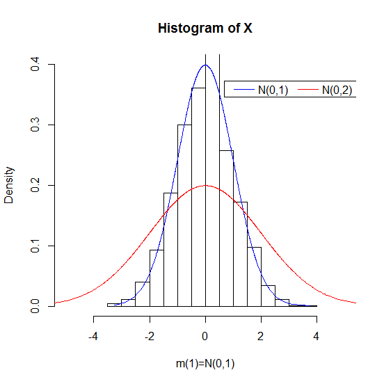
Figure 1: Histogram of ($DGP={\cal N}(0,1)$)

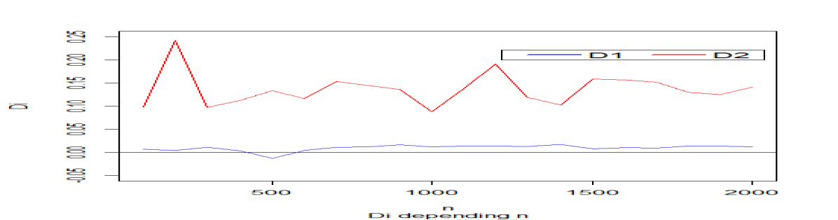
Figure 2: $\widehat{{\cal D}}_{1}$ and $\widehat{{\cal D}}_{2}$ depending $n$

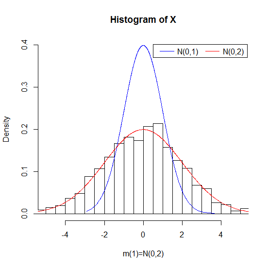
Figure 3: Histogram of ($DGP={\cal N}(0,2)$)

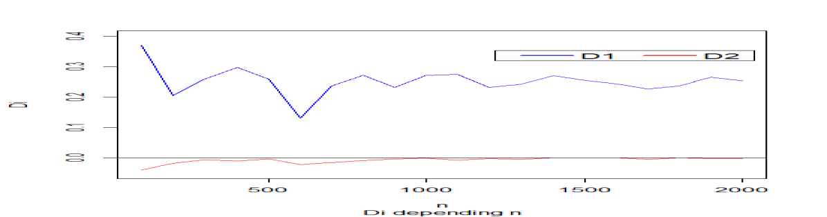
Figure 4: $\widehat{{\cal D}}_{1}$ and $\widehat{{\cal D}}_{2}$ depending $n$

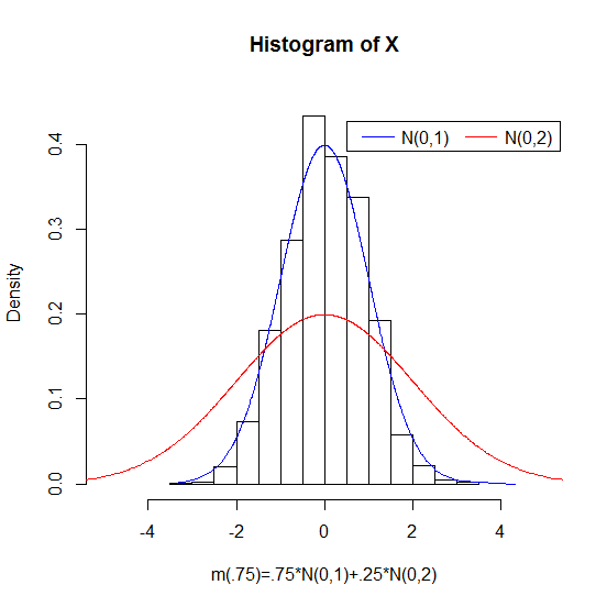
Figure 5: Histogram of ($DGP=.75*{\cal N}(0,1)+.25*{\cal N}(0,2)$)

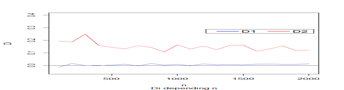
Figure 6: $\widehat{{\cal D}}_{1}$ and $\widehat{{\cal D}}_{2}$ depending $n$

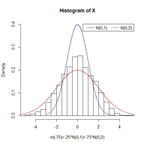
Figure 7: Coparaison barplot of Di depending n ($DGP=.25*{\cal N}(0,1)+.75*{\cal N}(0,2)$)

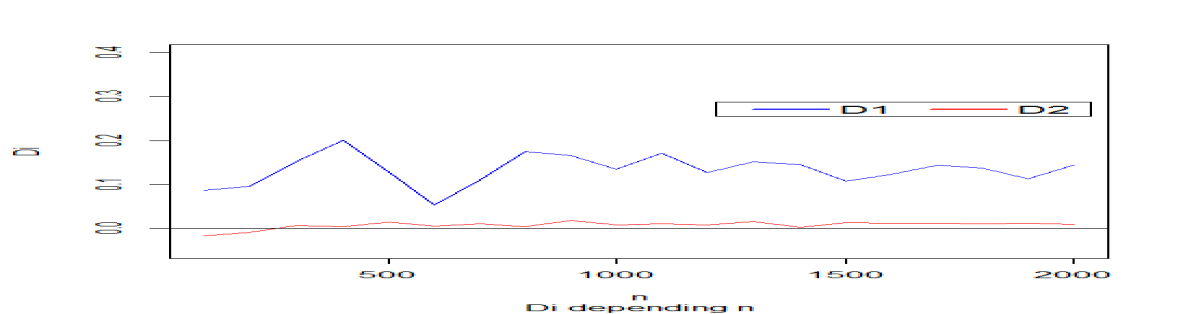
Figure 8: $\widehat{{\cal D}}_{1}$ and $\widehat{{\cal D}}_{2}$ depending $n$

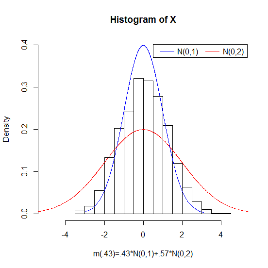
Figure 9: Coparaison barplot of Di depending n ($DGP=.43*{\cal N}(0,1)+.57*{\cal N}(0,2)$)

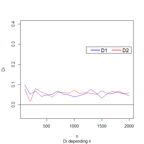
Figure 10: $\widehat{{\cal D}}_{1}$ and $\widehat{{\cal D}}_{2}$ depending $n$

In Figures 1, 3, 5 , 7 and 9 we plot the histograms of data sets and overlay the curves for ${\cal N}(0,1)$ and ${\cal N}(0,2)$ distribution. When the $DGP$ is correctly specified Figure 1, the ${\cal N}(0,1)$ distribution has reasonable chance of being distinguished from ${\cal N}(0,1)$ distribution.
Similarly, in Figure 3, as can be seen, the ${\cal N}(0,2)$ distribution closely approximates the data sets. In Figures 5 and 7 two distributions are close but the ${\cal N}(0,1)$ (Figure 5) and the ${\cal N}(0,2)$ distributions (Figure 7) does appear to be much closer to the data sets. When $\pi=0.43$, the distribution for both ( Figure 9) ${\cal N}(0,1)$ distribution and ${\cal N}(0,2)$ distribution are similar.

As expected, our statistic divergence $\widehat{{\cal DI}}_{\alpha}$ diverges to $-\infty$ (Figures 2 and 6) and to $+\infty$ (Figures 4 and 8) more rapidly symmetrical about the axis that passes through the mode of data distribution. This follows from the fact that these two distributions are equidistant from the fact that these two distributions are equidistant from the $DGP$ and would be difficult to distinguish from data in practice.
Figure 10 allows a comparison with the asymptotic ${\cal N}(0,\Gamma)$ approximation under our null hypothesis of equivalence.

6 conclusion

We learned a new nonparametric estimation for the Rényi$-\alpha$ and Tsallis$-\alpha$ divergence, and has been applied to problems of model selection. Under certain conditions, we have shown the consistency of these estimators and how they can be applied to estimate the distance between a known density and an unknown other than estimated by the kernel method. Our tests are based on testing whether the competing models are equally close to the true distribution against the alternative hypotheses that one model is closer than the other where closeness of a model is measured according to the discrepancy implicit in the divergence type statistics used. We have also demonstrated their effectiveness by using numerical experiments.

References

- [1] Alexander Bulinski and Alexey Shashkin. LIMIT THEOREMS FOR ASSOCIATED RANDOM FIELDS AND RELATED SYSTEMS.
- [2] Antonia Foldes. and Lidia Rejto, (1981). Strong Uniform Consistency for Nonparametric Survival Curve Estimators from Randomly Censored Data. Annals of Statistics. Volume 9, Number 1 (1981), 122-129.
- [3] Csiszr, I. (1967). Information-type measures of di?erences of probability distributions and indirect observations. Studia Sci. Math. Hungarica, 2:299318.
- [4] Deheuvels, P. and Einmahl, J. (1996). On the strong limiting behavior of local functionals of empirical processes based upon censored data. Ann. Prob. 24, 504 525.
- [5] Deheuvels, P. and Einmahl, J. (2000). Functional limit laws for the increments of kaplanmeier product-limit processes and applications. Ann. Prob.28(7), 1301 1335.
- [6] Diehl, S. and Stute, W. (1988). Kernel density and hazard function estimation in the presence of censoring. J. Mult. Analy.. 25, 299-310.
- [7] Lynda Atil. and Hocine Fellag. (2010). On the stability of the unit root test. Journal Afrika Statistika. Vol 5, 228-237.
- [8] Marriott, J. and Newbold, P. (1998). Bayesian comparison of ARIMA and stationary ARMA models. International Statistical Review. 66(3), 323-336.
- [9] Póczos, B. and Schneider, J.. On the estimation of alpha-divergences. CMU, Auton Lab Technical Report, http://www.cs.cmu.edu/ bapoczos/ articles/poczos11alphaTR.pdf.
- [10] Rényi, A. (1961). On measures of entropy and information. In Fourth Berkeley Symposium on Mathematical Statistics and Probability.
- [11] Rényi, A. (1970). Probability Theory. Publishing Company, Amsterdam.
- [12] Tanner, M. A. and Wong, W.H. (1983). The estimation of the hazard function from randomly censored data by the kernel method. Ann. Statist. 11, 989-993.
- [13] Villmann, T. and Haase, S. (2010). Mathematical aspects of divergence based vector quantization using Frechet-derivatives. University of Applied SciencesMittweida.
- [14] Watson, G.S. and M.R. Leadbetter, (1964a). Hazard Analysis I. Biometrika, Vol. 51, 1 and 2, pp. 175-184.
- [15] Watson, G.S. and M.R. Leadbetter, (1964b). Hazard Analysis II. Sankhya: The Indian Journal of Statistics, Series A, Vol. 26, No. 1, pp. 101-116.