Stable Roommates Problem with Random Preferences

Abstract

The stable roommates problem with $n$ agents has worst case complexity $O(n^{2})$ in time and space. Random instances can be solved faster and with less memory, however. We introduce an algorithm that has average time and space complexity $O(n^{\frac{3}{2}})$ for random instances. We use this algorithm to simulate large instances of the stable roommates problem and to measure the probabilty $p_{n}$ that a random instance of size $n$ admits a stable matching. Our data supports the conjecture that $p_{n}=\Theta(n^{-1/4})$.

Keywords: analysis of algorithms, typical-case computational complexity, interacting agent models, disordered systems (theory)

Published in: J. Stat. Mech. (2015) P01020

1 Introduction

Matching under preferences is a topic of great practical importance, deep mathematical structure, and elegant algorithmics [1, 2]. The most famous example is the stable marriage problem, where $n$ men and $n$ women compete with each other in the “marriage market.” Each man ranks all the women according to his individual preferences, and each woman does the same with all men. Everybody wants to get married to someone at the top of his or her list, but mutual attraction is not symmetric and frustration and compromises are unavoidable. A minimum requirement is a matching of men and women such that no man and woman would agree to leave their assigned partners in order to marry each other. Such a matching is called stable since no individual has an icentive to break it. The problem then is to find such a stable matching.

The stable marriage problem was introduced by David Gale and Lloyd Shapley in 1962 [3]. In their seminal paper they proved that each instance of the marriage problem has at least one stable solution, and they presented an efficient algorithm to find it. Since then, the Gale-Shapley algorithm has been applied to many real-world problems, not by dating agencies but by central bodies that organize two-sided markets like the assignment of students to colleges or residents to hospitals [4]. Besides its practical relevance, the stable marriage problem has many interesting theoretical features that have attracted researchers from various field, including physics [5, 6, 7, 8, 9].

The salient feature of the stable marriage problem is its bipartite structure: the agents form two groups (men and women), and matchings are only allowed between these groups but not within a group. This is adequate for two-sided markets. But what about one-sided markets, like the formation of cockpit crews from a pool of pilots or the assignment of students to the double bedrooms in a dormitory? The latter is known as the stable roommates problem. It is the paradigmatic example for matchings in one-sided markets.

The stable roommates problem was also introduced by Gale and Shapley [3]. They noted an intriguing difference between the marriage and the roommates problem: Whereas the former always has a solution, the latter may have none.

The Gale-Shapley algorithm for bipartite matching does not work for non-bipartite problems like the stable roommates problem. In fact some people believed that the roommates problem was NP-complete [10], but more than 20 years after the Gale-Shapley paper, Robert Irving presented a polynomial time algorithm for the stable roommates problem [11]. Irving’s algorithm either yields a stable solution or “No” if none exists.

An instance of the stable roommates problem consists of an even number $n$ of persons (students, pilots), each of whom ranks all of the others in strict order of preference. Since each person has to keep a list of preferences for all $n-1$ other persons, an instance of the stable roommates problem has size $\Theta(n^{2})$. Irving’s algorithm has time complexity $O(n^{2})$. This is optimal if we assume that one has to look at the complete instance (or at least a finite fraction of it) in order to solve the problem.

In this paper we show that in random instances, Irving’s algorithm only looks at $O(\sqrt{n})$ entries in each preference list, and we provide a modification of the algorithm that has average time and space complexity $O(n^{\frac{3}{2}})$. We use this algorithm to compute the probability $p_{n}$ that a random instance of size $n$ has a solution for systems that are more than $500$ times larger than previously simulated systems [12].

The paper is organized as follows. We start with a review of Irving’s algorithm. In Section 3 we discuss the complexity of Irving’s algorithm for random instances and our modification that reduces the average time and space complexity from $O(n^{2})$ to $O(n^{\frac{3}{2}})$. Section 4 comprises the results of the simulations on $p_{n}$, obtained with the modified algorithm.

2 The Algorithm

Irving’s algorithm can be expressed as a sequence of “proposals” from one person to another. If person $x$ makes a proposal to person $y$ (to share a room, to form a cockpit crew etc.), $y$ can accept or reject this proposal. If $y$ accepts the proposal, $x$ becomes semiengaged to $y$. If $y$ later receives another proposal from someone he prefers to $x$, he will accept the new proposal and cancel the semiengagement from $x$, who will in turn look for someone else to propose to.

As the name suggests, semiengagement is not symmetric: if $x$ is semiengaged to $y$, $y$ can be semiangaged to $z\neq x$ or to no one. If all semiengagements are symmetric, they represent a matching.

Irving’s algorithm proceeds in two phases. Phase I sets up semiengagements for everybody. In phase II, these semiengagements are modified by cyclically swapping partners until all semiengagements are symmetric, i.e., until they represent a matching. The corresponding sequence of proposals (and breakups) is organized such that the resulting matching is stable. If the instance admits no stable matching, this is recognized either in phase I or phase II by running out of partners to propose to.

For the time being, we assume that the preferences of all participants are stored in two 2-dimensional arrays:

• person[$x$,$i$]: person on position $i$ in $x$’s list,

• rank[$x$,$y$]: position of person $y$ in $x$’s list.

The two arrays are not independent, of course, but the redundancy allows us to look up persons and ranks in time $O(1)$.

For random instances we initialize the preference list of person $x$ a by random permutation of all other persons (including $x$) and then move $x$ to the very end of its own preference list. This means that we allow $x$ being matched with himself as the worst choice. If this really happens, this means that $x$ has no proper partner, i.e. that no stable matching exists for that instance.

In our implementation of the algorithm we will access the preference lists only through the function

function GetData($x$, $i$)

     $y$ := person[$x$, $i$]

     $r$ := rank[$y$, $x$]

     return ($y$, $r$)

end function

which returns the pair $(y,r)$ where $y$ is the person with rank $i$ in $x$’s prefence list and $r$ is rank of person $x$ in $y$’s preference list.

We will describe both phases of Irving’s algorithm without proving their correctness. For the proofs we refer the reader to Irving’s original paper [11].

2.1 Phase I

Phase I of the algorithm tries to establish semiengagements for every person. The general idea is that the first proposal of $x$ goes to the first person on his preference list, and only if this proposal is rejected (immediately or subsequently), $x$ proposes to the second person on his preference list and so on. On the receiving side, $y$ accepts a proposal only if the proposing person ranks higher on his preference list than the person whose proposal he has currently accepted.

Imagine the list of preferences written horizontally left (most desired partner) to right (least desired partner). Then the proposals made move from left to right, while the proposals accepted move from right to left. In a matching, both types of proposals meet at the same position. This motivates the names for the following lists that hold the current set of proposals:

• leftperson[$x$]: the person whom $x$ is currently proposing to,

• leftrank[$x$]: the rank of that person in $x$’s preference list,

• rightperson[$x$]: the person from which $x$ is currently holding a proposal

• rightrank[$x$]: the rank of that person in $x$’s preference list.

Again these lists are not independent, but the redundancy allows a faster lookup especially in phase II.

With this lists, the semiengagement of $x$ to $y$ is expressed by the simultaneous validity of the identities $y=\mbox{leftperson}[x]$ and $x=\mbox{rightperson}[y]$.

1:procedure Phase_I

2:     for $x:=1,\ldots,n$ do$\triangleright$ initialization

3:         $\mathrm{holds\_proposal}[x]:=\textbf{false}$$\triangleright$ no one is holding a proper proposal…

4:         $\mathrm{rightperson}[x]:=x$$\triangleright$ …but a proposal from self

5:         $\mathrm{rightrank}[x]:=n$$\triangleright$ self proposals are the worst

6:         $\mathrm{leftrank}[x]:=1$

7:     end for

8:     for $x:=1\ldots n$ do

9:         proposer := $x$

10:         repeat

11:              (next, rank) := GetData(proposer, leftrank[proposer])

12:              while rank $>$ rightrank[next] do

13:                  leftrank[proposer] := leftrank[proposer]+1

14:                  (next, rank) := GetData(proposer, leftrank[proposer])

15:              end while

16:              previous := rightperson[next]

17:              rightrank[next] := rank

18:              rightperson[next] := proposer

19:              leftperson[proposer] = next

20:              proposer := previous

21:         until holds_proposal[next] = false

22:         holds_proposal[next] := true

23:         if leftrank[proposer] = $n$ then $\triangleright$ proposer engaged to himself…

24:              return false $\triangleright$ … means: no stable matching possible

25:         end if

26:     end for

27:     return true

28:end procedure

Algorithm 1 Phase I of the stable roommates algorithm

Algorithm 1 shows the pseudocode for phase I of Irving’s algorithm. It stops, when every person holds a proposal, which implies that every person has also made a proposal that has been accepted, i.e. that every person is semiengaged. It returns false if someone has run out of partners (and is therefore engaged to himself), which means that there is no stable matching for this instance. If it returns true, we can still hope to find a stable matching in phase II of the algorithm.

2.2 Phase II

Phase I usually ends with everybody semiengaged to someone, but with asymmetric engagements $\mathrm{leftrank}[x]<\mathrm{rightrank}[x]$ for most persons $x$. Such persons have to give up their current proposal to leftperson[$x$] and find somebody down the list that would (temporarily) accept a proposal from $x$. We keep track of these second choices in the following lists

• secondperson[$x$]: $x$’s next best person that would accept a proposal

• secondrank[$x$]: the rank of that person in $x$’s preference list,

• secondrightrank[$x$]: the rank of $x$ in the preference list of secondperson[$x$].

If $x$ withdraws his proposal and proposes to $y=\mathrm{secondperson}[x]$, who temporarily accepts the proposal, the previous partners of $x$ and $y$ both loose their semiengagements and have to look themselves for their second best partners and so on. This avalanche of break-ups and new propsals is called a rotation. It reduces the difference rightrank[$x$]-leftrank[$x$] for several persons $x$ and is a step towards a matching.

The key idea of phase II is to organize this rearrangement of semiengagements in a so called all-or-nothing cycle. This is a sequence $a_{1}\ldots,a_{r}$ of persons such that $a_{i}$’s current second choice is $a_{i+1}$’s current first choice for $i=1\ldots,r-1$, and $a_{r}$’s current second choice is $a_{1}$’s current first choice. In terms of our lists, an all-or-nothing cycle is given by

$$\mathrm{secondperson}[a_{i}] = \mathrm{leftperson}[a_{i+1}]\quad i=1,\ldots,r-1$$

$$\mathrm{secondperson}[a_{r}] = \mathrm{leftperson}[a_{1}]\,.$$

In phase II of Irving’s algorithm, an all-or-nothing cycle is identified and the corresponding rotation is executed. This process is iterated until there are no more all-or-nothing cycles (in which case we’ve found a stable matching) or until someone runs out of partners after a rotation (in which case this instance has no stable matching).

1:procedure SeekCycle( )

2:     for $x:=1,\ldots,n$ do

3:         if $\mathrm{leftrank}[x]<\mathrm{rightrank}[x]$ then break $\triangleright$ find unmatched person

4:     end for

5:     if $\mathrm{leftrank}[x]\geq\mathrm{rightrank}[x]$ then $\triangleright$ no unmatched person found

6:         return ($0,0,\emptyset$)$\triangleright$ return empty cycle

7:     else$\triangleright$ unmatched person found

8:         $\mathrm{last}:=1$

9:         repeat

10:              $\mathrm{cycle}[\mathrm{last}]:=x$

11:              last := last + 1

12:              $p:=\mathrm{leftrank}[x]$

13:              repeat$\triangleright$ find second choice of $x$

14:                  $p:=p+1$

15:                  $(y,r):=$ GetData($x$, $p$)

16:              until $r\leq\mathrm{rightrank}[y]$$\triangleright$ $y$ would accept a proposal

17:              $\mathrm{secondrank}[x]:=p$$\triangleright$ store second choice

18:              $\mathrm{secondperson}[x]:=y$

19:              $\mathrm{secondrightrank}[x]:=r$

20:              $x:=\mathrm{rightperson}[\mathrm{secondperson}[x]]$$\triangleright$ next element in cycle

21:         until $x\in$ cycle $\triangleright$ cycle closed

22:         $\mathrm{last}:=\mathrm{last}-1$

23:         $\mathrm{first}:=\mathrm{last}-1$ $\triangleright$ rewind to start of cycle

24:         while cycle[first] $\neq x$ do $\mathrm{first}:=\mathrm{first}-1$

25:         return (first, last, cycle)

26:     end if

27:end procedure

Algorithm 2 Finding an all-or-nothing cycle for phase II of the stable roommates algorithm

Algorithm 2 shows the pseudocode for a function that finds and returns an all-or-nothing cycle or an empty cycle. To compute a cycle we need to identify the person whose current first choice is $y=\mathrm{secondperson}[x]$. But this person is simply given by $\mathrm{rightperson}[y]$, i.e., it can be found in time $O(1)$ (see line 20 of Alg. 2).

1:procedure Phase_II

2:     solution_possible := true

3:     solution_found := false

4:     while solution_possible and not solution_found do

5:         (first, last, cycle) := SeekCycle( )

6:         if cycle is empty then solution_found := true

7:         else

8:              for $x:=\mathrm{cycle}[\mathrm{first}],\ldots,\mathrm{cycle}[\mathrm{last}]$ do

9:                  $\mathrm{leftrank}[x]:=\mathrm{secondrank}[x]$

10:                  $\mathrm{leftperson}[x]:=\mathrm{secondperson}[x]$

11:                  $\mathrm{rightrank}[\mathrm{leftperson}[x]]:=\mathrm{secondrightrank}[x]$

12:                  $\mathrm{rightperson}[\mathrm{leftperson}[x]]=x$

13:              end for

14:              for $x:=\mathrm{cycle}[\mathrm{first}],\ldots,\mathrm{cycle}[\mathrm{last}]$ do

15:                  if $\mathrm{leftrank}[x]>\mathrm{rightrank}[x]$ then sol_possible := false

16:              end for

17:         end if

18:     end while

19:     return solution_found

20:end procedure

Algorithm 3 Phase II of the stable roommates algorithm

Algorithm 3 shows pseudocode for phase II which finds an all-or-nothing cycle, executes the corresponding rotation and iterates this until there are no more all-or-nothing cycles or a rotation has left a person without any partners to propose to.

The complete algorithm consists of an initialization phase (not shown), which generates a random preference list for each person, followed by calls to Phase_I and Phase_II.

3 Analysis and Modification

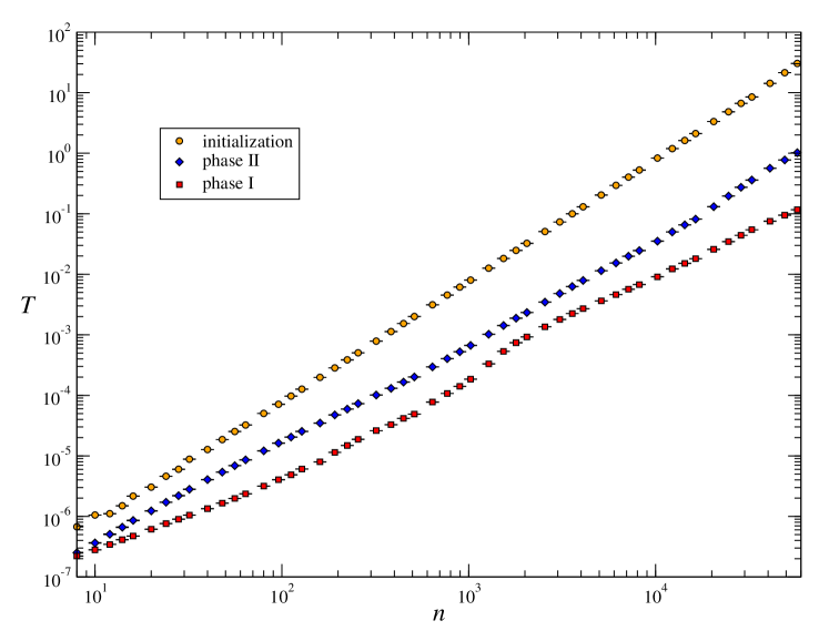
Figure 1: Running times of the various phases of Irving’s algorithm for random instances of the stable roommates problem. The total running time is dominated by the time for initialization of the complete instance. This time scales like $n^{2}$, whereas the time for the actual solution (phases I and II) grows much slower. The time $T$ is the average wallclock time in seconds on a single core of an Intel^® Xeon^® E5-1620 CPU running at 3.6 GHz. The “bump” in the data for phase I is probably due to cache misses for larger systems.

Figure 1 shows the average running times of the different phases on random instances of varying size $n$. The only phase that scales like $\Theta(n^{2})$ is the initialization, i.e., the generation of the random permutation of the preference lists. The time for the actual solution (phase I and phase II) grows significantly slower than $n^{2}$, which implies that the algorithm doesn’t need to look at the complete preference table to solve the problem.

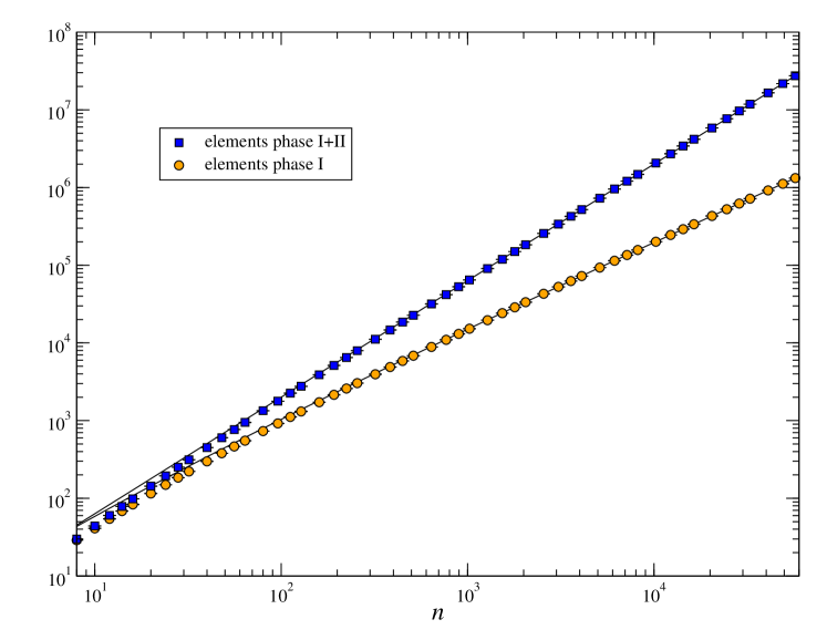
Figure 2: Number of elements in the preference tables that are actually read by Irving’s algorithm. Each symbol represents an average over $10^{4}$ random instances. The lines are $2n^{\frac{3}{2}}$ for the total number of elements and $2nH_{n}$ for phase I, where $H_{n}$ is the $n$th harmonic number.

Figure 2 shows the average number of entries in the preference lists that are actually read by Irving’s algorithm in order to find a stable matching or to report that no stable matching exists. For large values of $n$, this number is $2n^{\frac{3}{2}}$. This can be understood by the following simple, albeit non rigorous consideration. Let $k$ be the average number of proposals that a person makes in the course of Irving’s algorithm. Then $k$ is also the average number of proposals that a person receives, and the total number of entries in the preference table involved is $2kn$. Now $\mbox{leftrank}[x]$ increases by one with each proposal made by $x$, hence $\mbox{leftrank[$x$]}=k$ on average. The value of rightrank[$x$] is given by the minimum of $k$ values drawn uniformly from $1,\ldots,n$. Hence the distribution of $\mbox{rightrank}[x]=\ell$ is

$$P(\ell)=\frac{{{n-\ell}\choose{k-1}}}{{n\choose k}}\,,$$

with mean value $\frac{n+1}{k+1}$. The algorithm terminates if $\mbox{leftrank}[x]\simeq\mbox{rightrank}[x]$ or $k\simeq\frac{n+1}{k+1}$. Hence $k\simeq\sqrt{n}$, and the total number of entries read by Irving’s algorithm is $2n^{\frac{3}{2}}$. Note that this consideration ignores the fluctuations in rightrank[$x$]: if $k\simeq\sqrt{n}$, the standard deviation of $P(\ell)$ is $O(\sqrt{n})$, hence the number of proposals received by an individual person $x$ can differ considerably from the mean value $\sqrt{n}$. We do have the strict equality between the total number of proposals made and total number of proposals received, however. But a person, who has received more proposals than average, at termination has made less proposals than the average (and vice versa). Hence the individual fluctuations cancel in the total number of proposals if we assume, that at termination $\mbox{leftrank}[x]\simeq\mbox{rightrank}[x]$ for almost all persons $x$. This is not obvious, since in most cases (see next section) the algorithm terminates when the first person runs out of partners to propose to, i.e. the first time that $\mbox{leftrank}[x]>\mbox{rightrank}[x]$ for some $x$. It could well be that at that moment the gap between leftrank and rightrank is still large for some or many other persons. Hence the crucial assumption that underlies our argument is the assumption of a certain uniformity of the decrease of $\mbox{rightrank}[x]-\mbox{leftrank}[x]$ over all persons $x$. The fact that the observed total number of proposal is in fact narrowly concentrated around the predicted value (Figure  2) is an indication that this assumption is justified.

The number of elements read in phase I is even smaller. Phase I terminates if every person holds a proposal. Consider the sequence $x_{1},x_{2},\ldots$ of persons that receive a proposal. Phase I terminates if this sequence contains every person at least once. If we assume that the $x_{i}$’s are independent random variables, uniformly drawn from $\{1,\ldots,n\}$, this problem is known as the coupon collector’s problem [10]: an urn contains $n$ different coupons, and a collector draws coupons from that urn with replacement. How many coupons does the collector need to draw (on average), before he has drawn each coupon at least once? It is well known that the collector should expect to draw

$$n\,\left(1+\frac{1}{2}+\frac{1}{3}+\cdots+\frac{1}{n}\right)=nH_{n}$$

coupons in order to own at least one coupon of every kind. $H_{n}$ is known as the $n$th harmonic number. Note that

$$nH_{n}=n\,\log n+\gamma n+\frac{1}{2}+O(n^{-1})\,,$$ (1)

where $\gamma=0.5772156\ldots$ is the Euler-Mascheroni constant.

In our case, the $n$ coupons are the proposals to the $n$ different recipients, and phase I is the coupon collector. Hence the expected number of proposals in phase I is $nH_{n}$, and since each proposal implies two accesses to the preference lists, the number of elements read in phase I should be $2nH_{n}$. This is in fact the observed asymptotic scaling, as can be seen in Figure 2.

1:function GetData($x$, $i$)

2:     if $i\in$ rank[$x$] then$\triangleright$ element is known

3:         $y$ := person[$x$]($i$)

4:         $r$ := rank[$y$]($x$)

5:     else$\triangleright$ element is new

6:         repeat

7:              $y$ := random$\triangleright$ generate random person

8:         until $y\not\in$ person[$x$]

9:         repeat

10:              $r$ := random$\triangleright$ generate random rank

11:         until $r\not\in$ rank[$y$]

12:         $\mathrm{person}[x]:=\mathrm{person}[x]\cup(y,i)$$\triangleright$ save new table entries

13:         $\mathrm{rank}[x]:=\mathrm{rank}[x]\cup(i,y)$

14:         $\mathrm{person}[y]:=\mathrm{person}[y]\cup(x,r)$

15:         $\mathrm{rank}[y]:=\mathrm{rank}[y]\cup(r,x)$

16:     end if

17:     return ($y$,$r$)

18:end function

Algorithm 4 This version of the GetData function generates the entries of the preference lists “on the fly” as they are requested. The preference list of person $x$ is maintained in the associative arrays person[$x$] and rank[$x$].

We can exploit the fact that Irving’s algorithm looks only at $O(n^{3/2})$ elements of preference table by generating and storing only the elements that are requested by the algorithm. This saves us the expensive initialization phase and reduces the memory consumption considerably. Algorithm 4 shows the corresponding version of the function GetData. It maintains two arrays (person and rank) of maps. A map (aka associative array) is a data structure that holds pairs $(k,v)$ where $k$ is the key and $v$ is the value of the data element. In the map person[$x$], the key is the rank and the value is the person of that rank in $x$’s preference list. The map rank[$x$] holds the same data elements but with the role of key and value reversed. The rationale behind this redundancy is again efficiency: using hash tables, a map can be implemented such that the lookup of a value given the key can be done in (expected) constant time, independent of the number of elements. Hence GetData has average time complexity $O(1)$ when the requested data element is already known. When the requested element is new, the generation of a new random element may take longer since we need to generate a random person $y$ that is not contained in $x$’s preference list so far and an unoccupied rank $r$ for person $x$ in $y$’s list. Both are computed by a simple loop that generates random numbers until it hits a number not already contained in the list. In our case this is a reasonable approach since we know that the expected number of elements in person[$x$] and rank[$y$] is $O(\sqrt{n})$, hence the expected number of iterations in our loop is $1+O(n^{-1/2})$. Since inserting new elements in a map can also be done in constant time, the average time complexity of GetData is $O(1)$. Each map is initialized with the single entry person[$x$][$n$]=$x$ and rank[$x$][$x$]=$n$, all other entries are only added as needed.

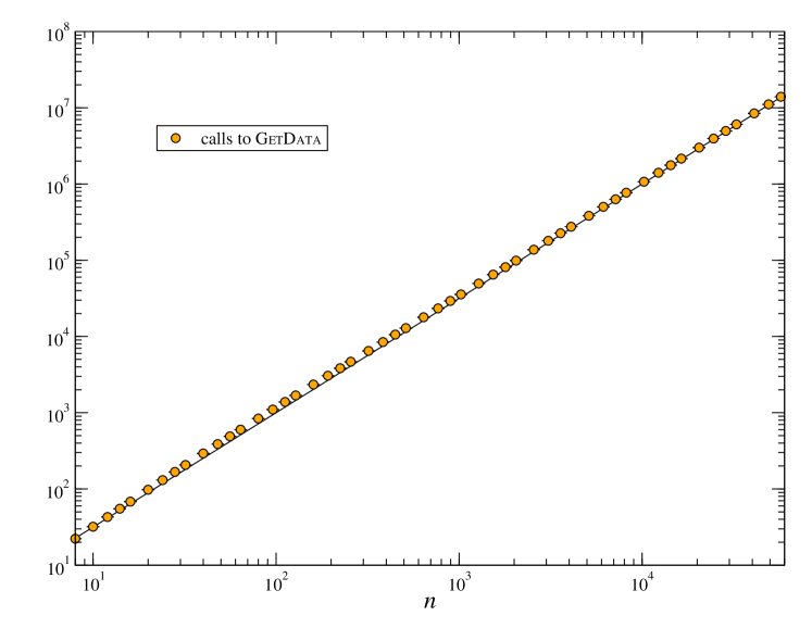
Figure 3: Number of calls of function GetData. Each symbol represents an average over $10^{4}$ random instances. The line is $n^{\frac{3}{2}}$.

The function GetData is called unconditionally from within the innermost loop in phase I. In phase II it is called for each element in search for a cycle (including all cycle elements). Hence the number of calls of GetData is a good measure for the average time complexity of the algorithm. As can be seen in Figure 3, the average time complexity is indeed $\Theta(n^{\frac{3}{2}})$.

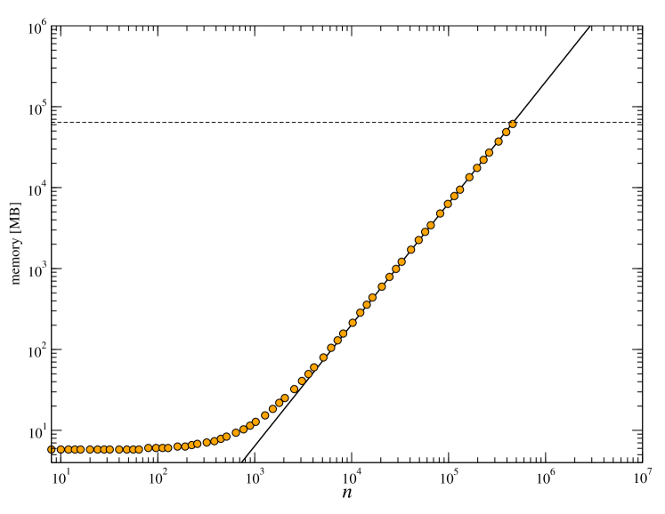
Figure 4: Actual memory consumption of Irving’s algorithm for random instances, implemented with associative maps. The solid line is a numerical $\Theta(n^{3/2})$ fit, the dashed line marks the 64 GBytes limit of our hardware.

The actual memory usage depends on the implementation of the map. We used the container class unordered_map from the C++ standard library provided by the GNU Compiler Collection (http://gcc.gnu.org). Figure 4 shows the total memory usage of the program. For large values of $n$ it is dominated by the maps person and rank and scales like $n^{3/2}$. On a computer with 64 GBytes of memory our implementation allows us to run problems up to $n\simeq 470\,000$, which is more than $5$ times larger than the maximum problem size allowed by a straightforward implementation with storage of the complete preference tables. The memory efficiency of our implementation is in fact so good that time becomes the bottleneck, as we will see in the next section.

4 Application

A long standing open problem is the computation of the probability $p_{n}$ that a random instance of the stable roommates problem of size $n$ has a stable matching [2, problem 8]. In particular one is interested in the asymptotic behavior of $p_{n}$ as $n$ grows large.

There is an integral representation for $p_{n}$ that can be used to compute $p_{n}$ exactly [13]. Unfortunately, the number of terms in the integral increases exponentially with $n^{2}$, which had limited the explicit evaluation of $p_{n}$ to the case $n=4$. Using a computer algebra system, we evaluated the integrals for $n\leq 10$ [14]:

$$p_{4} = \frac{26}{27}=0.96296\ldots$$

$$p_{6} = \frac{181431847}{194400000}=0.93329\ldots$$

$$p_{8} = {\frac{809419574956627}{889426440000000}}=0.910046\ldots$$

$$p_{10} = \frac{25365465754520943457921774207}{28460490127321448448000000000}=0.891251\ldots\,.$$

Computing $p_{n}$ for larger values of $n$ requires Monte Carlo simulations. These simulations indicate that $p_{n}$ is a monotonically decreasing function of $n$, but early simulations up to $n=2000$ [15] did not settle the question as to whether $p_{n}$ converges to $0$ or to some positive constant. The problem with simulations is that the decay of $p_{n}$ is rather slow. In fact Pittel [13] proved the asymptotic lower bound

$$p_{n}\gtrsim\frac{2\mathrm{e}^{3/2}}{\sqrt{\pi n}}$$ (2)

by applying the second moment method to the number of stable matchings. Extended simulations [12] up to $n=20000$ suggested an algebraic decay $p_{n}\simeq an^{-\delta}$. The numerical data from [12] was used to boldly conjecture the values of $a$ and $\delta$ as

$$p_{n}\simeq\mathrm{e}\sqrt{\frac{2}{\pi}}\,\,n^{-1/4}\,.$$ (3)

Using our algorithm with reduced running time and memory consumption, we can check this conjecture against extended numerical data.

We simulated systems of size $n=n_{0}2^{k}$, $k=0,\ldots,k_{\mathrm{max}}$ and $n_{0}\in\{8,10,12,14\}$ where $k_{\mathrm{max}}$ is limited by the available memory. In our case this means $k_{\mathrm{max}}\leq 15$ (Figure 4). The corresponding instances have an effective size that is more than $500$ times larger than the largest systems investigated in [12].

To measure $p_{n}$, we generate and solve $M$ independent random instances of size $n$ and record the fraction $\hat{p}_{n}$ of samples that admit a stable matching. The 95% confidence interval for $p_{n}$ is then $\hat{p}_{n}\pm 2\sigma_{n}$, where the standard deviation $\sigma$ is given by

$$\sigma_{n}=\sqrt{\frac{\hat{p}_{n}(1-\hat{p}_{n})}{M}}\,.$$ (4)

We vary the number of samples $M$ with the system size $n$. We used values from $M=10^{10}$ for small values of $n$ down to $M=10^{4}$ for the largest values of $n$. Table 1 shows the results.

$n$	$p_{n}$	$n$	$p_{n}$	$n$	$p_{n}$	$n$	$p_{n}$
8	0.910048(5)	128	0.60986(1)	2048	0.32473(9)	32768	0.1650(4)
10	0.891247(6)	160	0.58183(1)	2560	0.30794(9)	40960	0.1563(4)
12	0.875525(6)	192	0.55946(1)	3072	0.29464(9)	49152	0.1494(3)
14	0.861952(6)	224	0.54099(1)	3584	0.28391(9)	57344	0.1440(5)
16	0.849958(7)	256	0.52536(1)	4096	0.27486(9)	65536	0.140(2)
20	0.829239(7)	320	0.49993(1)	5120	0.26042(9)	81920	0.132(2)
24	0.811499(7)	384	0.47987(1)	6144	0.2492(2)	98304	0.126(2)
28	0.795768(7)	448	0.46339(2)	7168	0.2402(2)	114688	0.120(2)
32	0.781542(8)	512	0.44949(2)	8192	0.2320(2)	131072	0.118(2)
40	0.756482(8)	640	0.42704(2)	10240	0.2200(2)	163840	0.111 (2)
48	0.734851(8)	768	0.40939(7)	12288	0.2103(2)	196608	0.103(6)
56	0.715866(8)	896	0.39482(7)	14336	0.2024(3)	229376	0.104(6)
64	0.699044(9)	1024	0.38270(9)	16384	0.1961(3)	262144	0.098(6)
80	0.670377(9)	1280	0.36327(9)	20480	0.1854(4)	327680	0.097(6)
96	0.646797(9)	1536	0.34782(9)	24576	0.1774(4)	393216	0.089(6)
112	0.62692(1)	1792	0.33526(9)	28672	0.1709(4)	458752	0.085(5)

Table 1: Values of $p_{n}$ from simulations. Notation: $p_{8}=0.910048(5)$ means that $[0.910048-0.000005,0.910048+0.000005]$ is the 95% confidence interval for $p_{8}$.

We ran our simulation on a small cluster consisting of five nodes. Each node has 64 GByte of RAM and two Intel Xeon CPU E5-2630 running at 2.30GHz. Each CPU has 6 real cores or (using hpyerthreading) 12 virtual cores. For smaller systems, we can use all $5\times 2\times 12=120$ virtual cores to solve instances in parallel, but for the larger sizes, the available memory per core limits the number of usable cores. The available memory allows us to compute problems up to $n=2^{15}\times 14=458752$ using only one core per node. Solving a single instance of this size takes about 14 minutes, i.e. solving a sample of $M=10^{4}$ instances as in Table 1 takes about 20 days on $5$ nodes in parallel.

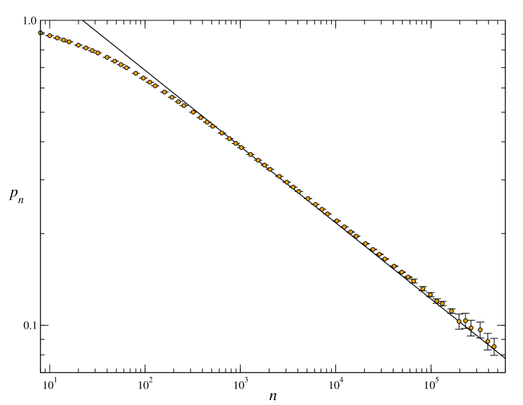
Figure 5: Simulation results for $p_{n}$ in a log-log-plot. Error bars denote 95% confidence intervals. The line represents the conjectured asymptotic behavior (3).

Figure 5 shows $p_{n}$ versus $n$ in a log-log-plot. The data supports an asymptotic algebraic decay $p_{n}\simeq an^{-\delta}$ for some constants $\delta$ and $a$, in agreement with the conjecture (3), which is also displayed in Figure 5. The visual impression suggests that $\delta=1/4$ as claimed in (3), but that the true prefactor $a$ is slightly larger than $\mathrm{e}\sqrt{2/\pi}$. In fact, a least squares fit of the one-parameter function $a\,n^{-1/4}$ to the data points for $n\geq 32765$ yields $a=2.223(3)$, which is 3% larger than $\mathrm{e}\sqrt{2/\pi}=2.1688\ldots$.

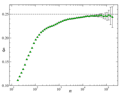
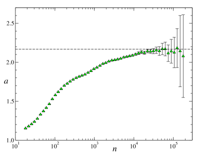
Figure 6: Results of a least-squares fit of $p_{n}=an^{-\delta}$ to a sliding window of $w=10$ consecutive data points. The abscissa represents the geometric mean of the $n$-values contained in a window.

The numerical value of the fit parameter varies with the choice of the data points used in the least square fit, however. As a more systematic way to estimate the asymptotic behavior we applied least squares fitting of the two-parameter function $an^{-\delta}$ to sliding windows of $w$ consecutive data points $p_{n}$. Figure 6 shows the results for $w=10$. Larger values of $w$ yield similar curves with smaller errorbars but fewer data points. This analysis shows that the available numerical data for $p_{n}$ supports the conjecture (3) within the errorbars.

A more elementary question is whether $\lim_{n\to\infty}p_{n}$ is zero or non-zero. To address this question we applied the sliding window technique to fit the three parameter function $p_{n}=an^{-\delta}+b$. The result for $b$ is a curve very similar to the curves shown in Figure 6 with $b$ converging to zero within the errorbars. This result supports the claim $\lim_{n\to\infty}p_{n}=0$.

5 Conclusions and Outlook

We have demonstrated that Irving’s algorithm for the stable roommates problem can be organized such that the expected time and space complexity is $O(n^{3/2})$ on random instances. Our reasoning about the dynamics of the algorithm (approaching random walks of leftrank and rightrank, phase I as coupon collector’s problem) is of course non-rigorous, but the results are well confirmed by the numerical simulations. Maybe this simplistic view on Irving’s algorithm can help to derive the observed $n^{-1/4}$ decay of the probability $p_{n}$ that a random instance of size $n$ has a solution.

References

References

- [1] David F. Manlove. Algorithmics of Matching under Preferences, volume 2 of Series on Theoretical Computer Science. World Scientific, Singapore, 2013.
- [2] Dan Gusfield and Robert W. Irving. The Stable Marriage Problem: Structure and Algorithms. The MIT Press, Cambridge, Massachusetts, 1989.
- [3] David Gale and Lloyd S. Shapley. College admissions and the stability of marriage. American Mathematical Monthly, 69:9–15, 1962.
- [4] Alvin E. Roth and Marilda A. Oliveira Sotomayor. Two-sided matching: A study in game-theoretic modeling and analysis. Economic Society Monographs. Cambridge University Press, 1990.
- [5] Marie-José Oméro, Michael Dzierzawa, Matteo Marsili, and Yi-Cheng Zhang. Scaling behavior in the stable marriage problem. Journal de Physique I, 7(12):1723–1732, 1997.
- [6] Theo M. Nieuwenhuizen. The marriage problem and the fate of bachelors. Physica A: Statistical and Theoretical Physics, 252(1–2):178–198, 1998.
- [7] Michael Dzierzawa and Marie-José Oméro. Statistics of stable marriages. Physica A: Statistical and Theoretical Physics, 287:321–333, 2000.
- [8] Guido Caldarelli and Andrea Capocci. Beauty and distance in the stable marriage problem. Physica A: Statistical and Theoretical Physics, 300:325–331, 2001.
- [9] Alejandro Lage-Castellanos and Roberto Mulet. The marriage problem: from the bar of appointments to the agency. Physica A: Statistical Mechanics and its Applications, 364:389–402, May 2006.
- [10] Cristopher Moore and Stephan Mertens. The Nature of Computation. Oxford University Press, 2011. www.nature-of-computation.org.
- [11] Robert W. Irving. An efficient algorithm for the stable roommates problem. J. Algorithms, 6:577–595, 1985.
- [12] Stephan Mertens. Random stable matchings. J. Stat. Mech., 2005(10):P10008, 2005.
- [13] Boris Pittel. The ”stable roommates” problem with random preferences. Ann. Probab., 21(3):1441–1477, 1993.
- [14] Stephan Mertens. Small random instances of the stable roommates problem. In preparation.
- [15] Boris Pittel and Robert W. Irving. An upper bound for the solvability of a random stable roommates instance. Random Struct. Algorithms, 5(3):465–487, 1994.