Adapting to a Changing Environment: Non-Obvious Thresholds in Multi-Scale Systems

Abstract

Many natural and technological systems fail to adapt to changing external conditions and move to a different state if the conditions vary too fast. Such “non-adiabatic” processes are ubiquitous, but little understood. We identify these processes with a new nonlinear phenomenon—an intricate threshold where a forced system fails to adiabatically follow a changing stable state. In systems with multiple timescales, we derive existence conditions that show such thresholds to be generic, but non-obvious, meaning they cannot be captured by traditional stability theory. Rather, the phenomenon can be analysed using concepts from modern singular perturbation theory: folded singularities and canard trajectories, including composite canards. Thus, non-obvious thresholds should explain the failure to adapt to a changing environment in a wide range of multi-scale systems including: tipping points in the climate system, regime shifts in ecosystems, excitability in nerve cells, adaptation failure in regulatory genes, and adiabatic switching in technology.

Keywords

rate-induced bifurcations, canards, folded singularity, thresholds

I Introduction

The time evolution of real-world systems often takes place on multiple timescales, and is paced by aperiodically changing external conditions. Of particular interest are situations where, if the external conditions change too fast, the system fails to adapt and moves to a different state. In climate science and ecology one speaks of “rate-induced tipping points” Wieczorek2010 ; Lenton2008 ; Stocker1997 ; Leemans2004 , the “critical rate hypothesis” Scheffer2008 , and “adaptation failure” Bridle2007 to describe the sudden transitions caused by too rapid changes in external conditions (e.g. dry and hot climate anomalies or wet periods due to El Niño-Southern Oscillation). In neuroscience, type III excitable nerves (Izhikevich2007, , Ch. 7) accommodate slow changes in an externally applied voltage, but an excitation requires a rapid enough increase in the voltage Hill1936 ; Biktashev2002 . In nonequilibrium genetic circuits, cells are forced to decide between alternative fates in response to changing extracellular conditions, and the decision is determined by the rate of change Nene2012 . However, such rate-induced transitions cannot, in general, be explained by traditional stability theory, and require an alternative approach.

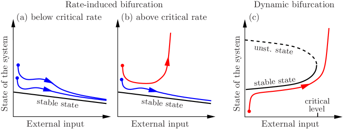
Figure 1: (Colour online) The conceptual difference between (a)–(b) a rate-induced bifurcation and (c) a dynamic bifurcation in systems with a time-varying external input. The “stable state” is an asymptotic stable state when the external input is fixed in time. In (a)–(b), a response to a varying external input is (red) non-adiabatic, meaning the system destabilises, or (blue) adiabatic, meaning the system tracks the moving stable state.

This paper conceptualises the failure to adapt to a changing environment as a rate-induced bifurcation Wieczorek2010 ; Ashwin2012 —a non-autonomous instability characterised by critical rates of external forcing Wieczorek2010 ; Ashwin2012 and instability thresholds Wieczorek2010 ; Mitry2013 . Rate-induced bifurcations can be counter-intuitive because they occur in systems where a stable state exists continuously for all fixed values of the external input [Fig. 1(a)–(b)]. When the external input varies in time, the position of the stable state changes and the system tries to keep pace with the changes. The forced system adiabatically follows or tracks the continuously changing stable state if the external input varies slowly enough [Fig. 1(a)]. However, many systems fail to track the changing stable state if the external input varies too fast. These systems have initial states that destabilise—move away to a different, distant state—above some critical rate of forcing [Fig. 1(b)]. This happens even though there is no obvious loss of stability. Moreover, in systems with multiple timescales there may be no obvious threshold separating the adiabatic and non-adiabatic responses in Fig. 1(b). This is in contrast to dynamic bifurcations Lobry1991 , which can be explained by classical bifurcations of the stable state at some critical level of external input [Fig. 1(c)]. In this case, the forced system destabilises totally predictably around the critical level, independently of the initial state and of the rate of change.

In the absence of an obvious threshold, scientists are often puzzled by the actual boundary separating initial states that adapt to changing external conditions from those that fail to adapt. The first non-obvious threshold was identified only recently, in the context of a rate-induced climate tipping point termed the “compost-bomb instability”, as a folded saddle canard Wieczorek2010 . This finding explained a sudden release of soil carbon from peat lands into the atmosphere above some critical rate of warming, which puzzled climate carbon-cycle scientists Luke2011 ; Wieczorek2010 . Subsequently, similar non-obvious “firing thresholds” explained the spiking behaviour of type III neurons Mitry2013 ; Wechselberger2014 .

Here, we reveal a non-obvious threshold with an intricate band structure, and discuss the underlying mathematical mechanism. The uncovered threshold is generic, and should explain the failure to adapt to a changing environment in a wide range of nonlinear multi-scale systems. Specifically, the intricate band structure is shown to arise from a combination of the complicated dynamics due to a folded node singularity Szmolyan2001 and the simple threshold behaviour due to a folded saddle singularity Wieczorek2010 near a folded saddle-node type I Krupa2010 ; Guckenheimer2008 ; Vo2014 . What is more, the threshold is identified with special composite canards—trajectories that follow canard segments of different folded singularities. More generally, we derive existence results for critical rates and non-obvious thresholds, and discuss our contribution in the context of canard theory and its applications.

II A general framework and existence results for non-obvious thresholds

Our general framework is based on geometric singular perturbation theory Fenichel1979 ; Jones1995 . It builds on the ideas developed in Wieczorek2010 , and extends the analysis to any type of smoothly varying external input. Specifically, we consider multi-scale dynamical systems akin to simple climate, neuron, and electrical circuit models Luke2011 ; Wieczorek2010 ; Roberts2013 ; Cessi1994 ; Mitry2013 ; Wechselberger2014 ; Pol1934 :

$$\delta\;dx/dt = f(x,y,\lambda(\epsilon t),\delta),$$ (1)

$$dy/dt = g(x,y,\lambda(\epsilon t),\delta),$$ (2)

with a fast variable $x$, slow variable $y$, and sufficiently smooth functions $f$ and $g$. The small parameter $0<\delta\ll 1$ quantifies the ratio of the $x$ and $y$ timescales. The time-varying external input $\lambda(\epsilon t)$ is bounded between $\lambda_{\min}$ and $\lambda_{\max}$, and evolves smoothly on a slow timescale

$$\tau=\epsilon t,$$

where $\tau\in(\tau_{\min},\tau_{\max})$ can be unbounded.

The system has two small parameters: $\delta$ and $\epsilon$. While the analysis of rate-induced bifurcations is greatly facilitated by the singular limit $\delta=0$, it requires nonzero $\epsilon$. The limit $\epsilon=0$ gives the conceptual starting point for the analysis.

When $\lambda$ does not vary in time, i.e. when $\epsilon=0$, Eqs. (1)–(2) define a dynamical system with one fast and one slow variable, and a parameter $\lambda$. In the singular limit $\delta=0$, the slow subsystem $dy/dt=g(x,y,\lambda,0)$ evolves on the one-dimensional critical manifold $S(\lambda)$, defined by $f(x,y,\lambda,0)=0$. Alternatively, $S(\lambda)$ consists of steady states of the fast subsystem $dx/dT=f(x,y,\lambda,0)$, where $T=t/\delta$ is the fast timescale, and $y$ acts as a second parameter. The critical manifold can have an attracting part $S^{a}(\lambda)$ and a repelling part $S^{r}(\lambda)$, which are separated by a fold point $F(\lambda)$ (Fig. 2). To give precise statements about non-obvious thresholds we assume for every fixed $\lambda$ between $\lambda_{\min}$ and $\lambda_{\max}$:
(A1) The system has a quadratic nonlinearity. The critical manifold $S(\lambda)$ is locally a graph over $x$ with a single fold $F(\lambda)$ tangent to the fast $x$-direction, defined by

$$\frac{\partial f}{\partial x}\Big{|}_{S}=0\quad\mbox{and}\quad\frac{\partial^{2}f}{\partial x^{2}}\Big{|}_{S}\neq 0.$$ (3)

(A2) The system has a stable state for all fixed external conditions. Near $F(\lambda)$, $S^{a}(\lambda)$ contains just one steady state $\tilde{x}(\lambda)$ which is asymptotically stable and varies continuously with $\lambda$.
The geometric structure of the phase space in the singular limit $\delta=0$ gives insight into the dynamics for $\delta$ small, but nonzero. Specifically, where steady states of the fast subsystem are hyperbolic (i.e. on $S^{a}(\lambda)$ and $S^{r}(\lambda)$ but not on $F$), system (1)–(2) with $0<\delta\ll 1$ has a slow attracting manifold $S^{a}_{\delta}(\lambda)$ and a slow repelling manifold $S^{r}_{\delta}(\lambda)$. Both $S^{a}_{\delta}(\lambda)$ and $S^{r}_{\delta}(\lambda)$ are locally invariant, lie close to, and have the same stability type as $S^{a}(\lambda)$ and $S^{r}(\lambda)$, respectively. This follows from Fenichel’s Theorem Fenichel1979 ; Jones1995 .

When $\lambda$ varies smoothly in time such that $0<\epsilon\lesssim 1$ and $0<\delta\ll 1$, Eqs. (1)–(2) define a dynamical system with one fast and two slow variables:

$$\delta\epsilon\;dx/d\tau = f(x,y,\lambda(\tau),\delta),$$ (4)

$$\epsilon\;dy/d\tau = g(x,y,\lambda(\tau),\delta),$$ (5)

$$d\tau/d\tau = 1.$$ (6)

Now the critical manifolds $S^{a}$ and $S^{r}$, as well as the slow manifolds $S^{a}_{\delta}$ and $S^{r}_{\delta}$ are two-dimensional, and $\tilde{x}$ and $F$ form curves (Fig. 2). When $\lambda(\tau)$ varies slowly enough, the forced system (1)–(2) tracks the continuously changing stable state $\tilde{x}(\lambda(\tau))$. However, the system may fail to track, and destabilise. To be more precise, we define:
Definition 1. For a given initial state on $S^{a}_{\delta}$, we say that system (1)–(2) destabilises if the trajectory leaves $S^{a}_{\delta}$ and moves away along the fast $x$-direction. Otherwise, we say that system (1)–(2) tracks the moving stable state $\tilde{x}(\lambda(\tau))$.
Definition 2. The critical rate $\epsilon_{c}$ is the largest $\epsilon$ below which there are no initial states on $S^{a}_{\delta}$ that destabilise.
Definition 3. The instability threshold is the boundary within $S^{a}_{\delta}$ separating initial states that track $\tilde{x}(\lambda(\tau))$ from those that destabilise.
Figure 2 (a)–(b) shows two trajectories of Eqs. (1)–(2) for different initial states on $S^{a}$. Below the critical rate, all trajectories track, and eventually converge to $\tilde{x}(\lambda(\tau))$ [Fig. 2(a)]. However, above the critical rate there are initial states near $\tilde{x}$ that fail to track $\tilde{x}(\lambda(\tau))$, and the system destabilises [red in Fig. 2(b)]. Interestingly, some trajectories leave $S^{a}_{\delta}$ but, instead of destabilising along the fast $x$-direction, return to $S^{a}_{\delta}$ and converge to $\tilde{x}$ [blue in Fig. 2(b)]. The two qualitatively different behaviours in Fig. 2(b) show there is an instability threshold within $S^{a}_{\delta}$. What is more, the threshold can be simple [Fig. 2(c)] as reported in Wieczorek2010 ; Mitry2013 , or can have an intriguing band structure [Fig. 2(d)] that has not been reported to date. In both cases, it is not immediately obvious what determines the threshold.

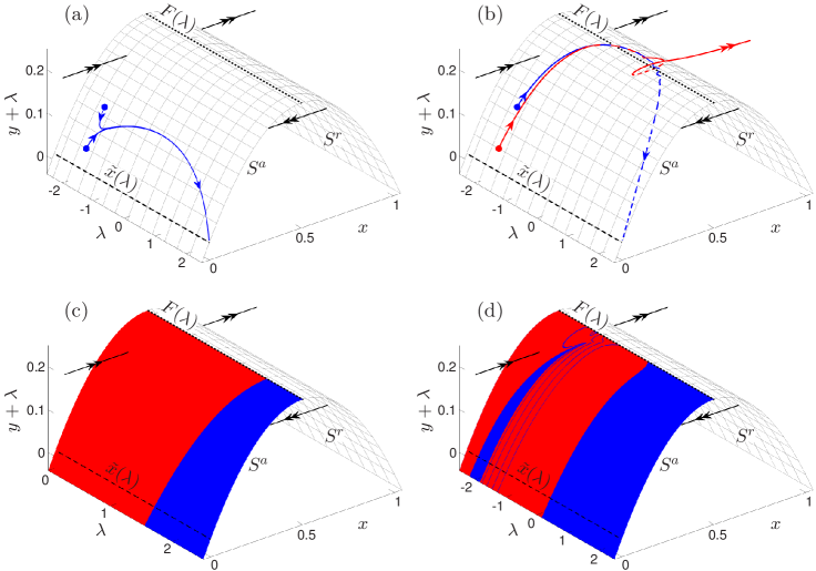
Figure 2: (Colour online) (a)–(b) Trajectories starting at two different initial states (dots) on $S^{a}$, near the changing stable state $\tilde{x}$, (a) below and (b) above the critical rate. (c)–(d) Above the critical rate, the initial states on $S^{a}$ that (red) destabilise or (blue) track $\tilde{x}(\lambda(\tau))$ highlight different threshold types. We used Eqs. (1)–(2), (13), and [(a), (b), (d)] Eq. (14) with (a) $\epsilon=0.06$ and [(b), (d)] $\epsilon=0.216$; and (c) Eq. (19) with $\epsilon=1$. Other parameters were $\delta=0.01$, $\lambda_{\max}=2.5$. For (a)–(d) the critical manifold $S(\lambda)$ is given by $y=-\lambda-x(x-1)$, has a fold $F(\lambda)$ at $(x,y)=(1/2,-\lambda+1/4)$ and a unique stable steady state $\tilde{x}(\lambda)$ at $(x,y)=(0,-\lambda)$. For clarity, the plots are shown in the co-moving coordinate system $(x,y+\lambda,\lambda)$. The $\lambda$ axis can be transformed into a slow time axis using [(a), (b), (d)] Eq. (14) or (c) Eq. (19).

The analysis of the mathematical mechanism for non-obvious thresholds is greatly facilitated by the singular limit $\delta=0$, where the fold and slow manifolds are unique and known exactly. System (4)–(6) is reduced to the slow dynamics on $S$ by setting $\delta=0$, and then projected onto the $(x,\tau)$-plane by differentiating Eq. (4) with respect to slow time $\tau$:

$$dx/d\tau = -\frac{g\,\partial f/\partial y+\epsilon(\partial f/\partial\lambda)(d\lambda/d\tau)}{\epsilon\,\partial f/\partial x}\Big{|}_{S},$$ (7)

$$d\tau/d\tau = 1.$$ (8)

It now becomes clear that if a trajectory deviates too much from $\tilde{x}$ and approaches a typical point on $F$ then, according to fold condition (3), $\partial f/\partial x$ in Eq. (7) approaches zero, and $x$ diverges off to infinity in finite slow time $\tau$. However, there may be special points on $F$ where

$$\left[g\,\partial f/\partial y+\epsilon(\partial f/\partial\lambda)(d\lambda/d\tau)\right]|_{F}=0,$$ (9)

and $dx/d\tau$ remains finite. Such special points are referred to as folded singularities Takens1976 ; Szmolyan2001 . The corresponding trajectories, that cross from $S^{a}$ along the eigendirections of a folded singularity onto $S^{r}$, are referred to as singular canards Szmolyan2001 . The distinction between systems that have a critical rate and those that do not appears to be whether there are trajectories started on $S^{a}$ that reach $F$ away from a folded singularity, or whether all trajectories started on $F$ flow onto $S^{a}$. Furthermore, canard trajectories, being solutions that separate these two behaviours, are candidates for non-obvious thresholds.

An obstacle to the analysis of critical rates and instability thresholds is that the flow on $F$, specifically the right hand side of Eq. (7), is not well defined. This obstacle can be overcome by a special time rescaling Dumortier1996 :

$$d\tau=-ds\;\epsilon\,\left.(\partial f/\partial x)\right|_{S},$$

where the new time $s$ passes infinitely faster on $F$, and reverses direction on $S^{r}$:

$$\lim_{(x,\tau)\to F}\frac{ds}{d\tau}=\left\{\begin{array}[]{r l}\infty&\text{ if }(x,\tau)\in S^{a},\\ -\infty&\text{ if }(x,\tau)\in S^{r}.\end{array}\right.$$

This gives the desingularised system

$$dx/ds = \left.[g\,\partial f/\partial y+\epsilon\,(\partial f/\partial\lambda)(d\lambda/d\tau)]\right|_{S},$$ (10)

$$d\tau/ds = -\epsilon\,\left.(\partial f/\partial x)\right|_{S},$$ (11)

where trajectories remain the same as in Eqs. (7)–(8), the vector field on $F$ becomes well defined, folded singularities become regular steady states, and singular canards become trajectories tangent to an eigenspace of a steady state. One speaks of “folded nodes”, “folded saddles” and “folded foci” for Eqs. (7)–(8) if a steady state for Eqs. (10)–(11) has real eigenvalues with the same sign, real eigenvalues with opposite signs, and complex eigenvalues with nonzero real parts, respectively. Most importantly, the difference between tracking and destabilising can easily be analysed using Eqs. (10)–(11). Specifically, we derive conditions for the existence of critical rates and non-obvious thresholds:
Theorem 1. Existence of critical rates: a dissipative Adiabatic Theorem. Suppose the forced system (1)–(2) with assumptions (A1)–(A2) satisfies the folded singularity condition (9) for some $\tau\in(\tau_{\min},\tau_{\max})$ and $\epsilon>0$. Then, system (1)–(2) has a critical rate $\epsilon_{c}$. The critical rate is approximately the largest $\epsilon$ below which (9) is never satisfied within $(\tau_{\min},\tau_{\max})$:

$$\epsilon_{c}\approx\inf\left\{\epsilon>0:\left[g\,\partial f/\partial y+\epsilon(\partial f/\partial\lambda)(d\lambda/d\tau)\right]|_{F}=0\right\}.$$

Theorem 2. Existence of non-obvious thresholds. The forced system (1)–(2) with assumptions (A1)–(A2) is guaranteed to have an instability threshold if a folded saddle is the only folded singularity within $(\tau_{\min},\tau_{\max})$. Then, the threshold is given by the folded saddle maximal canard. If $\tau_{\max}=\infty$ and $\lambda(\tau)$ is asymptotically constant

$$\lim_{\tau\to\infty}\frac{d\lambda}{d\tau}=0,$$ (12)

then the system has an instability threshold if, and only if, there is a folded saddle singularity.
Note. Often in real-life applications the changing external conditions $\lambda$ are expressed as a prescribed function of time $t$, but not $\epsilon$ or $\tau$. Specifying $\epsilon$ is not necessary. If one replaces $\tau$ with $\epsilon t$ in Eqs. (4)–(11) the dependence on $\epsilon$ disappears. However, $\epsilon$ and $\tau$ are useful for defining critical rates of change, and facilitate the derivation of the statements in Theorems 1 and 2.

The proofs, given in the Appendix, are based on two steps. In the first step, a qualitative analysis of Eqs. (10)–(11) identifies the appearance of a folded singularity with a critical rate, and certain singular canards as candidates for an instability threshold. In the second step, recent results from canard theory Szmolyan2001 ; Wechselberger2005 ; Vo2014 are used that state singular canards due to folded saddles, folded nodes, and folded saddle-nodes of type I, perturb to maximal canards in (4)–(6) with $0<\delta\ll 1$. Maximal canards are those trajectories crossing from $S^{a}_{\delta}$ onto $S^{r}_{\delta}$, which remain on $S^{r}_{\delta}$ for the longest time. In this paper, we numerically compute both maximal canards $\gamma_{\delta}$, shown in Fig. 4, and their approximations by singular canards $\gamma$, shown in Figs. 3 and 5.

III Two cases of a non-obvious threshold

Guided by the proof of Theorem 2, specifically the analysis of the phase portraits containing a folded saddle [Appendix, Fig. 6(a)–(b)], we distinguish two cases of a non-obvious threshold. Furthermore, we identify one case with the complicated threshold shown in Fig. 2(d), and uncover the underlying mechanism.

We illustrate the two cases using an example of (1)–(2) with

$$f=x(x-1)+y+\lambda(\tau)\;\;\;\mbox{and}\;\;\;g=-x,$$ (13)

and two different aperiodic forcing functions $\lambda(\tau)$ satisfying (12).

Case 1: Complicated threshold due to a folded saddle-node type I singularity. Consider example (13) subject to logistic growth at a rate $\epsilon$:

$$\lambda(\tau)=\lambda_{\max}\,\tanh\!\left(\tau\right),$$ (14)

where $\lambda\in(-\lambda_{\max},\lambda_{\max})$, $\tau\in(-\infty,\infty)$ and $\tau=\epsilon t$. The desingularised system (10)–(11) becomes

$$dx/ds = -x+\frac{\epsilon}{\lambda_{\max}}\left(\lambda_{\max}^{2}-\lambda^{2}(\tau)\right),$$ (15)

$$d\tau/ds = \epsilon(1-2x).$$ (16)

Steady states of (15)–(16) lie on the fold $x=1/2$, at $\lambda(\tau)$ satisfying the folded singularity condition (9):

$$\lambda^{2}(\tau)-\lambda_{\max}\left(\lambda_{\max}-\frac{1}{2\epsilon}\right)=0,$$ (17)

and their eigenvalues $\xi$ are found from the characteristic polynomial

$$\xi^{2}+\xi-4\epsilon^{2}\lambda(\tau)\left[1-\left(\frac{\lambda(\tau)}{\lambda_{\max}}\right)^{2}\right]=0.$$ (18)

The folded singularity condition (17) has no real roots when $\epsilon<(2\lambda_{\max})^{-1}$. When $\epsilon=(2\lambda_{\max})^{-1}$, there is a double root within $(\tau_{\min},\tau_{\max})$, corresponding to a folded saddle-node type I Krupa2010 at $(x,\lambda(\tau))=(1/2,\,0)$. When $\epsilon>(2\lambda_{\max})^{-1}$, there are two distinct roots within $(\tau_{\min},\tau_{\max})$, corresponding to a stable folded node (focus) $FN(FF)$ at $(x,\lambda(\tau))=(1/2,\,-\sqrt{\lambda_{\max}(\lambda_{\max}-(2\epsilon)^{-1})}\,)$ and a folded saddle $FS$ at $(x,\lambda(\tau))=(1/2,\,\sqrt{\lambda_{\max}(\lambda_{\max}-(2\epsilon)^{-1})}\,)$. This means that, upon increasing $\epsilon$, there is a generic saddle node bifurcation of folded singularities at $\epsilon_{SN}=(2\lambda_{\max})^{-1}$, which by Theorem 1 is approximately the critical rate $\epsilon_{c}$ for $0<\delta\ll 1$. According to Theorem 2, condition (12) and the presence of a folded saddle guarantee an instability threshold. However, unlike the case of an isolated folded saddle whose threshold is specified by Theorem 2, it is not immediately clear what forms the threshold near a folded saddle-node type I Vo2014 . Nonetheless, this can be established numerically.

The instability threshold is defined on the attracting slow manifold $S^{a}_{\delta}$, which is difficult to compute near the fold $F$. To facilitate numerical computations, we consider initial states on the critical manifold $S^{a}$, which is known exactly. The results are shown in Fig. 3, where the white regions indicate destabilising, and the grey regions indicate tracking. Away from $F$, the critical manifold $S^{a}$ closely approximates the slow manifold $S^{a}_{\delta}$. Here, the instability threshold is well approximated by the boundaries between the white and grey regions. However, caution is required near $F$, especially around $FN$, where $S^{a}_{\delta}$ twists in a complicated manner (Desroches2012, , Fig. 6), and the chosen surface of initial conditions, $S^{a}$, intersects these twists. There, the boundaries between the white and grey regions deviate from the instability threshold due to the choice of initial states. We also show what happens to initial states on $S^{r}$ just to the right of $F$, as some are mapped along the fast flow onto $S^{a}_{\delta}$ and converge to $\tilde{x}$. This is why a “reflection” of the band structure from $S^{a}$ can be seen on $S^{r}$.

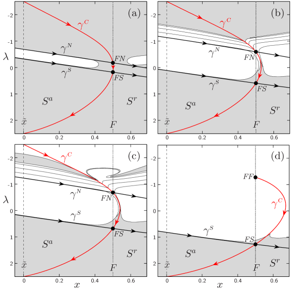
Figure 3: (Colour online) Initial states on the critical manifold $S$ that (white) destabilise or (grey) track $\tilde{x}(\lambda(\tau))$ in Eqs. (1)–(2) and (13)–(14) with $\delta=0.01$, $\lambda_{\max}=2.5$, and $\epsilon=\mbox{(a)}\,0.201,\,\mbox{(b)}\,0.212,\,\mbox{(c)}\,0.216,\,\mbox{and (d)}\,0.270$, shown projected onto the $(x,\lambda)$ plane. Away from $F$, the instability threshold in $S^{a}_{\delta}$ is well approximated by the white-grey boundary in $S^{a}$. Points $FN$, $FS$, and $FF$ are folded node, folded saddle, and folded focus singularities, respectively; the strong folded node singular canard $\gamma^{N}$ and the folded saddle singular canard $\gamma^{S}$ approximate projections of the maximal canards $\gamma^{N}_{\delta}$ and $\gamma^{S}_{\delta}$, respectively, onto $S$. The projection of the maximal canard $\gamma^{C}_{\delta}$ onto $S$ is approximated by the weak folded node/faux saddle singular canard $\gamma^{C}$ when $\lambda>-1$, but lies below $\gamma^{C}$ for $-2.5<\lambda<-1$, e.g. within the wide grey band around $\lambda=-2$ in (c). Although it is difficult to see, $\gamma^{C}$ terminates on $F$ just above $FF$. Compare (c) with Fig. 2(d).

Shortly past the saddle-node bifurcation, there are three bands of initial states on $S^{a}$ [Fig. 3(a)]. The threshold separating these bands is formed by two canard trajectories: the folded saddle maximal canard $\gamma^{S}_{\delta}$, and the strong folded node maximal canard $\gamma^{N}_{\delta}$. On $S^{a}$, trajectories started in the white band enclosed by $\gamma^{S}_{\delta}$ and $\gamma^{N}_{\delta}$ move directly towards the fold, then leave the attracting slow manifold $S^{a}_{\delta}$ and destabilise along the fast $x$-direction. Trajectories started in the grey band below $\gamma^{S}_{\delta}$ approach the faux saddle maximal canard $\gamma^{C}_{\delta}$ straight away, thereby staying on the attracting slow manifold $S^{a}_{\delta}$ and tracking $\tilde{x}$. This is in contrast to trajectories started in the other grey band on $S^{a}$, the one above $\gamma^{N}_{\delta}$. These trajectories initially approach and twist around the weak folded node maximal canard $\gamma^{C}_{\delta}$, and leave $S^{a}_{\delta}$. However, rather than destabilising, they are fed back along $\gamma^{C}_{\delta}$, onto $S^{a}_{\delta}$, and eventually remain on $S^{a}_{\delta}$ [Fig. 2(b), blue trajectory]. Finally, grey initial states on $S^{r}$ are mapped along the fast flow onto the grey bands on $S^{a}_{\delta}$.

As $\epsilon$ increases, the threshold becomes more complicated due to the presence of the stable folded node $FN$. Additional threshold curves appear successively above $\gamma^{N}_{\delta}$, giving up to five white bands of initial states above $\gamma^{N}_{\delta}$ that destabilise [Fig. 3(b)]. Trajectories started within these additional white bands twist around $\gamma^{C}_{\delta}$ before destabilising, [Fig. 2(b), red trajectory]. These white bands are separated by narrow grey bands which are difficult to see in Fig. 3; see the narrow grey band in the inset of Fig. 4, or narrow blue bands in Fig. 2(d). Trajectories started within these narrow grey bands leave $S^{a}_{\delta}$, follow a maximal canard on $S^{r}_{\delta}$ for some time, but then return to $S^{a}_{\delta}$ into the grey region below $\gamma^{S}_{\delta}$, and converge to $\tilde{x}$. The white bands expand with $\epsilon$ and approach the weak folded node maximal canard $\gamma^{C}_{\delta}$ on both sides [Fig. 3(c)]. When the folded node $FN$ turns into a folded focus $FF$ at $\epsilon=(2+\sqrt{4+\lambda_{\max}^{2}}\,)/8\lambda_{\max}$, its canards disappear Szmolyan2001 and so does the band structure [Fig. 3(d)]. We are left with a simple threshold, given just by $\gamma^{S}_{\delta}$ as in Ref. Wechselberger2014 .

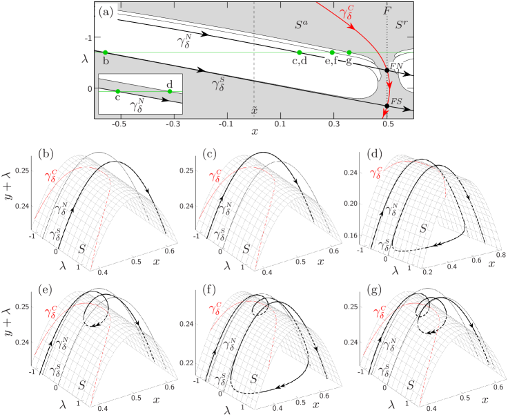
Figure 4: (Colour online) (a) Initial states on the critical manifold $S$ that (white) destabilise or (grey) track $\tilde{x}(\lambda(\tau))$ in Eqs. (1)–(2) and (13)–(14) with $\delta=0.01$ and $\epsilon=0.204$. Inset shows grey band between c and d; a similar band exists between e and f. Labels b–g at $\lambda=-0.7$, or $\tau=-\tanh^{-1}(0.28)$, denote different threshold components including: (b) the folded saddle maximal canard $\gamma^{S}_{\delta}$, (c) the strong folded node maximal canard $\gamma^{N}_{\delta}$, (d) a composite canard that follows $\gamma^{N}_{\delta}$ and $\gamma^{S}_{\delta}$, (e) a secondary folded node maximal canard, (f) a composite canard that follows a secondary maximal canard and $\gamma^{S}_{\delta}$, (g) a secondary folded node maximal canard.

The key mechanism for complicated thresholds is the phenomenon whereby trajectories leave $S^{a}_{\delta}$ through the folded node region and then, rather than destabilising, are fed back to $S^{a}_{\delta}$ through the folded saddle region. This phenomenon has two consequences. Firstly, not all initial states on $S^{a}_{\delta}$ and above $\gamma^{N}_{\delta}$ destabilise. Secondly, the initial states on $S^{a}_{\delta}$ that destabilise or track $\tilde{x}$ form alternating bands, and these bands have not been identified before. More generally, the alternating bands are related to the known rotational sectors of a folded node; see Wechselberger2005 for a detailed discussion of rotational sectors. However, whilst rotational sectors are separated by a single canard trajectory Desroches2012 ; Wechselberger2005 , our white bands are separated by a narrow grey band bounded by two different canard trajectories.

Figure 4 identifies the different components of the complicated threshold. They consist of known maximal canards such as (b) $\gamma^{S}_{\delta}$, (c) $\gamma^{N}_{\delta}$, and [(e) and (g)] secondary folded node maximal canards that bifurcate off $\gamma^{C}_{\delta}$ Wechselberger2005 . These canards form the lower boundaries of the narrow grey bands. Most interestingly, they also consist of new composite canards that follow canard segments of different folded singularities. These canards form the upper boundaries of the narrow grey bands. Figure 4 shows composite canards which initially (d) follow $\gamma^{N}_{\delta}$, or (f) follow the first secondary folded node maximal canard, and then [(d) and (f)] follow $\gamma^{S}_{\delta}$. This explains the intriguing band structure with intermingled regions of white and grey in Figs. 3(b)-(c) and 4(a), or red and blue in Fig. 2(d). The composite canards in Fig. 4(d) and (f) are reminiscent of trajectories that switch between different primary and secondary canards of the same folded node in a stellate cell model Wechselberger2009 and in a reduced Hodgkin-Huxley model (Desroches2010, , Fig. 9).

Case 2: Simple threshold due to an isolated folded saddle singularity. Consider example (13) subject to an exponential approach at a rate $\epsilon$:

$$\lambda(\tau)=\lambda_{\max}\left(1-e^{-\tau}\right),$$ (19)

where $\lambda\in(0,\lambda_{\max})$, $\tau\in(0,\infty)$ and $\tau=\epsilon t$. The desingularised system (10)–(11) becomes

$$dx/ds = -x+\epsilon\left(\lambda_{\max}-\lambda(\tau)\right),$$ (20)

$$d\tau/ds = \epsilon(1-2x).$$ (21)

The steady state of (20)-(21) lies on the fold $x=1/2$, at $\lambda(\tau)$ satisfying the folded singularity condition (9):

$$\lambda(\tau)=\lambda_{\max}-\frac{1}{2\epsilon},$$ (22)

and its eigenvalues $\xi$ are found from the characteristic polynomial

$$\xi^{2}+\xi+2\epsilon^{2}\left(\lambda(\tau)-\lambda_{\max}\right)=0.$$ (23)

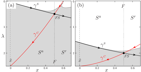
Figure 5: (Colour online) Initial states on the critical manifold $S$ that (white) destabilise or (grey) track $\tilde{x}(\lambda(\tau))$ for Eqs. (1)–(2), (13), and (19) with $\delta=0.01$, $\lambda_{\max}=2.5$, and (a) $\epsilon=0.25$, (b) $\epsilon=1$, shown projected onto the $(x,\lambda)$ plane. Away from $F$ the instability threshold in $S^{a}_{\delta}$ is well approximated by the white-grey boundary in $S^{a}$. Compare (b) with Fig. 2(c). For labels see Fig. 3.

The main difference from Case 1 is that the different forcing $\lambda(\tau)$ in (19) gives a folded singularity condition (22) with just a single root, corresponding to an isolated folded saddle $FS$ at $(x,\lambda(\tau))=(1/2,\,\lambda_{\max}-(2\epsilon)^{-1})$. Upon increasing $\epsilon$, the folded saddle enters $(\tau_{\min},\tau_{\max})$ via its lower boundary when $\epsilon=(2\lambda_{\max})^{-1}$, which by Theorem 1 is approximately the critical rate $\epsilon_{c}$ for $0<\delta\ll 1$. According to Theorem 2, there is an instability threshold given by the folded saddle maximal canard $\gamma^{S}_{\delta}$, as in the compost-bomb and the type III neuron examples Wieczorek2010 ; Mitry2013 . Numerical computations in Fig. 5 confirm that for $\delta=0.01$, and away from $F$, the threshold is well approximated by the singular canard $\gamma^{S}$. It is interesting to note, the threshold in Fig. 5 is very similar to that in Fig. 3(d).

Note on types of non-obvious thresholds. Theorem 2 in conjunction with numerical investigations in this section show that which case of a non-obvious threshold occurs, if any at all, depends both on the system (1)–(2) and the form of the external input $\lambda(\tau)$. Specifically, the threshold is determined by the number, type and stability of the folded singularities. What is more, our simple example (13) demonstrates that both cases of a non-obvious threshold can occur for the same system when subject to different $\lambda(\tau)$.

In both cases, the external input $\lambda(\tau)$ satisfies (12). When $\lambda(\tau)$ does not satisfy (12), there can be an instability threshold that is not associated with a folded saddle [Appendix, Fig. 6(d)]. However, it follows from the proof of Theorem 2 in the Appendix that such a threshold is simple, akin to the case of an isolated folded saddle.

IV Conclusions

In summary, we analysed multiple timescale systems subject to an aperiodically changing environment, identified nonlinear mechanisms for the failure to adapt, and derived conditions for the existence of these mechanisms. Specifically, we discussed instability thresholds where a system fails to adiabatically follow a continuously changing stable state. Despite their cross-disciplinary nature, these thresholds are largely unexplored because they are “non-obvious”, meaning they cannot, in general, be revealed by traditional stability theory. Thus, they require an alternative approach. We presented a framework, based on geometric singular perturbation theory, that led us to a novel type of threshold with an intriguing band structure. The threshold has alternating bands, where the system tracks the moving stable state, or destabilises. We showed that this structure is organised by a folded saddle-node type I singularity. Intuitively, it arises from an interplay of the complicated dynamics of twisting canard trajectories due to a folded node singularity, and the simple threshold behaviour illustrated for a folded saddle singularity. Most importantly, trajectories which leave the attracting slow manifold through the folded node region can be fed back to the attracting slow manifold through the folded saddle region. In more technical terms, the band structure is related to the rotational sectors of a folded node, but also differs from them in one key aspect. Whereas the rotational sectors are separated by a single canard trajectory, namely the maximal canard Desroches2012 ; Wechselberger2005 , the corresponding wide bands are separated by a narrow band. These separating narrow bands are bounded by two different canard trajectories. One of them is a known maximal canard, and the other is a composite canard that follows maximal-canard segments of different folded singularities.

Whilst non-obvious thresholds can be complicated, they are generic, and should explain counter-intuitive responses to a changing environment in a wide range of multi-scale systems. We highlighted their importance by examples of climate and ecosystems failing to adapt to a rapidly changing environment Wieczorek2010 ; Ashwin2012 ; Luke2011 , and type III excitable cells “firing” only if the voltage stimulus rises fast enough Mitry2013 ; Hill1936 . More generally, our results give new insight into non-adiabatic processes in multi-scale dissipative systems, and should stimulate further work in canard theory.

Appendix

Consider system (1)–(2) with assumptions (A1)–(A2), and restrict the discussion to $\tau\in(\tau_{\min},\tau_{\max})$, which can be unbounded.

Proof of Theorem 1.

Let $p$ be a point on the fold $F$ in the desingularised system (10)–(11). By (A1) the vector field at $p$ only has a component in the $x$-direction. When $\epsilon=0$, by assumption (A2) the vector field points towards the attracting critical manifold $S^{a}$ at every $p\in F$. This means all trajectories starting on $F$ flow onto $S^{a}$, and no trajectories starting on $S^{a}$ reach $F$. When $\epsilon>0$, there may be trajectories that reach $F$ from $S^{a}$. This happens if, and only if, the vector field changes sign at some $p\in F$ as $\epsilon$ is varied:

$$(dx/ds)|_{p} = \left.[g\,\partial f/\partial y+\epsilon\,(\partial f/\partial\lambda)(d\lambda/d\tau)]\right|_{p}=0,$$ (24)

$$\frac{d}{d\epsilon}(dx/ds)\Big{|}_{p} = [(\partial f/\partial\lambda)(d\lambda/d\tau)]|_{p}\neq 0.$$ (25)

Furthermore, by assumption (A1) $S$ can be expressed as a graph over $y$ meaning $(\partial f/\partial y)|_{p}\neq 0$, and by assumption (A2) there are no steady states on $F$ in the full system meaning $g|_{p}\neq 0$, so (24) already implies (25).

By (Jones1995, , Th. 1), if system (10)–(11) has no trajectories started on $S^{a}$ that reach $F$, then system (4)–(6) has no trajectories that leave $S^{a}_{\delta}$ for $0<\delta\ll 1$. Furthermore, by (Szmolyan2004, , Th. 1), if system (4)–(6) has trajectories starting on $S^{a}$ that reach $F$ away from a folded singularity, then system (4)–(6) has trajectories that leave $S^{a}_{\delta}$ and move away along the fast $x$-direction for $0<\delta\ll 1$. Hence, the folded singularity condition (24) implies a critical rate for system (4)–(6), and for the original system (1)–(2).

By Definition 2, in the singular limit $\delta=0$ the critical rate is the largest $\epsilon$ below which (24) is never satisfied within $(\tau_{\min},\tau_{\max})$. When $\delta$ is small but nonzero, the critical rate is given by

$$\epsilon_{c}\approx\inf\left\{\epsilon>0:\left[g\,\partial f/\partial y+\epsilon(\partial f/\partial\lambda)(d\lambda/d\tau)\right]|_{F}=0\right\}+E_{\delta},$$

where $E_{\delta}$ is a correction for nonzero $\delta$. For $\delta$ small enough, the correction term $E_{\delta}$ is $O({\delta}^{\frac{1}{2}})$ if the folded singularity at $\epsilon_{c}$ is a saddle, node, or folded saddle-node type II Szmolyan2001 ; Krupa2010 , and is $O({\delta}^{\frac{1}{4}})$ if the folded singularity at $\epsilon_{c}$ is a folded-saddle node type I Vo2014 .

Proof of Theorem 2.

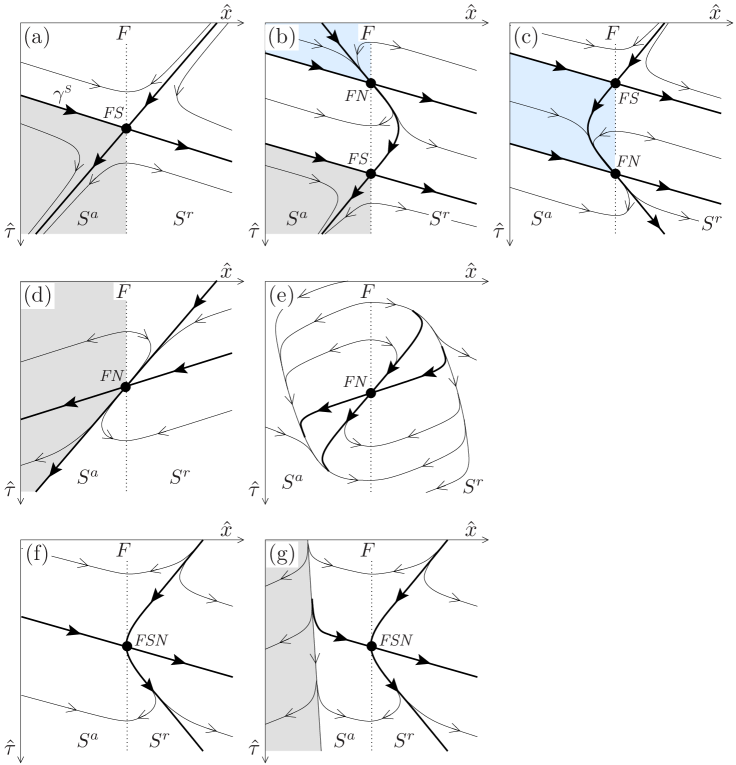
Figure 6: (Colour online) Sketches of selected phase portraits for system (7)-(8), containing folded saddles ($FS$), folded nodes ($FN$), and folded saddle-nodes ($FSN$). Singular canards are shown in bold. On $S^{a}$, there are trajectories that (white) approach $F$ away from a folded singularity, (blue) leave $S^{a}$ via a folded singularity, and (grey) never reach $F$.

Consider a fixed value of $\epsilon>\epsilon_{c}$. We are interested in phase portraits of system (7)–(8) which have two types of trajectories starting on $S^{a}$: those that reach $F$ away from a folded singularity, and those that never reach $F$ and remain on $S^{a}$. We refer to the separatrix dividing these two types of trajectories as the singular threshold. Phase portraits of system (7)–(8) that may contain a singular threshold are identified as follows. We keep in mind that $d\tau/dt>0$, construct possible phase portraits of the desingularised system (10)–(11), reverse the flow on $S^{r}$, and keep those portraits that allow a singular threshold.

The proof consists of three parts. Firstly, we analyse an arbitrary external input $\lambda(\tau)$ to show that an isolated folded saddle guarantees a singular threshold. Secondly, we analyse an asymptotically constant external input, i.e. $\lambda(\tau)$ satisfies condition (12), to show there is a singular threshold if, and only if, there is a folded saddle. Lastly, we use recent results from canard theory to show that singular thresholds persist as instability thresholds for $\delta$ small, but nonzero.

Part 1

Firstly, assume condition (9) is satisfied, meaning there is a folded singularity $p$. Without loss of generality, suppose $p$ is at the origin. According to (Szmolyan2001, , Prop. 2.1), under assumption (A1) and condition (9), there is a smooth change of coordinates that projects the fold curve $F$ orthogonally onto the $\tau$-axis and, in the neighbourhood of $p$, brings the desingularised system (10)–(11) to the normal form

$$\frac{d\hat{x}}{d\hat{s}} = b\hat{\tau}+c\hat{x}+O(\hat{x}^{2},\hat{x}\hat{\tau},\hat{\tau}^{2}),$$ (26)

$$\frac{d\hat{\tau}}{d\hat{s}} = -2\epsilon\hat{x}+O(\hat{x}^{2},\hat{x}\hat{\tau}),$$ (27)

where $\hat{x}$ and $\hat{\tau}$ are the new coordinates, the fold $F$ is defined by $\hat{x}=0$, and the attracting critical manifold $S^{a}$ is defined by $\hat{x}<0$. The eigenvalues of $p$:

$$\xi_{1,2}=(c\pm\sqrt{c^{2}-8\epsilon b}\,)/2,$$

determine the type of the folded singularity in system (7)–(8). In particular, $p$ is a folded saddle if $b<0$, a folded saddle-node if $b=0$, and a folded node, focus or centre if $b>0$. The key observation for our purposes is that $b\neq 0$ determines the direction of the flow on $F$ where $d\hat{\tau}/d\hat{s}=0$ and $d\hat{x}/d\hat{s}=b\hat{\tau}+O(\hat{\tau}^{2})$.

In the case of a folded saddle ($b<0$), trajectories starting on $S^{a}$ and near $F$ reach $F$ when $-1\ll\hat{\tau}<0$, or flow away from $F$ onto $S^{a}$ when $0<\hat{\tau}\ll 1$ [Fig. 6(a)]. If a folded saddle is the only folded singularity, then there are no additional changes in the direction of the flow on $F$. The local behaviour for $0<\hat{\tau}\ll 1$ extends to $0<\hat{\tau}<\hat{\tau}_{\max}$, meaning no trajectories started on $S^{a}$ for $\hat{\tau}>0$ ever reach $F$. Hence, an isolated folded saddle implies a singular threshold. What is more, the threshold is given by the singular folded saddle canard. This can be seen by noting that, in the desingularised system (10)–(11), the separatrix between trajectories starting on $S^{a}$ that reach $F$ and those that never reach $F$ is the stable manifold of the saddle equilibrium. This stable manifold becomes the singular folded saddle canard $\gamma_{\delta}^{S}$ in system (7)–(8) [Fig. 6(a)]. If, in addition to a folded saddle, there are other folded singularities, a singular threshold can no longer be guaranteed [e.g. Fig. 6(c)], nor excluded [e.g. Fig. 6(b)]. To obtain the threshold, one needs to study the behaviour of trajectories started on $S^{a}$; see the analysis of Case 1 in Section 3.

In the special case of a folded saddle-node ($b=0$), the flow on $F$ in system (26)–(27) is determined by $d\hat{x}/d\hat{s}=O(\hat{\tau}^{2})$. This means there is no change in the sign of the flow at $p$ [e.g. Fig. 6(f)]. A folded saddle-node is structurally unstable. Under arbitrarily small variation of system parameters, it unfolds into a folded saddle at positive $\hat{\tau}$ and a folded node at negative $\hat{\tau}$ (multiple singularities discussed in the paragraph above), or into no singularities. In the case of a folded node, focus or centre ($b>0$), trajectories starting on $S^{a}$ and sufficiently close to $F$ flow away from $F$ onto $S^{a}$ when $-1\ll\hat{\tau}<0$, or reach $F$ when $0<\hat{\tau}\ll 1$; see an example of an unstable folded node in Fig. 6(d). For $b\geq 0$, a singular threshold cannot be guaranteed [e.g. Fig. 6(f)–(g)], nor excluded [e.g. Fig. 6(d)–(e)].

Secondly, assume there are no folded singularities. If the flow on $F$ in system (26)–(27) points towards $S^{a}$, a singular threshold can be excluded. If the flow on $F$ points towards $S^{r}$, a singular threshold cannot be guaranteed, nor excluded [restricting the $(\hat{\tau}_{\min},\hat{\tau}_{\max})$ interval to the lower part of the phase portrait in Fig. 6(d) gives a singular threshold without a folded singularity].

Finally, if $\hat{\tau}_{\max}$ is positive and finite, there may be ‘spurious’ singular thresholds in phase portraits with a folded singularity and $b\geq 0$, or with no folded singularities, where all trajectories starting on $S^{a}$ and near $F$ for $\hat{\tau}>0$ flow towards $F$. However, because $\hat{\tau}_{\max}$ is finite, some of these trajectories will simply fail to reach $F$ by $\hat{\tau}_{\max}$.

It turns out that many examples of a singular threshold described above, including the ‘spurious’ singular threshold, can be eliminated with a sensible assumption about $\lambda(\tau)$.

Part 2

A more definitive statement about instability thresholds can be made when $\tau_{\max}=\infty$, and the external input is asymptotically constant, i.e. $\lambda(\tau)$ satisfies condition (12).

Assume there is a singular threshold. On the one hand, it follows from assumption (A1) and from condition (12) that, for sufficiently large ${\tau}$, trajectories started on $S^{a}$ and near $F$ must flow onto $S^{a}$ and approach $\tilde{x}$. On the other hand, a singular threshold requires trajectories that start on $S^{a}$ and reach $F$. Hence, the flow on $F$ in the desingularised system (10)–(11) must point towards $S^{a}$ for large values of $\tau$, and towards $S^{r}$ for lower values of $\tau$. Such a change in the direction of the flow on $F$ requires a folded singularity with $b>0$ in (26)–(27). Hence, a folded saddle is necessary for a singular threshold.

Assume there is a folded saddle singularity. There are two possible situations. First, a folded saddle is the only folded singularity. Second, a folded saddle is one of many folded singularities. In the second situation, assumption (A1) and condition (12) require that, typically, the folded singularity with the largest $\tau$-component is a folded saddle. “Typically” excludes a folded saddle-node which is not structurally stable. In both situations, there is a singular threshold by the argument used for an isolated folded saddle in Part 1 of this proof. Hence, a folded saddle is sufficient for a singular threshold.

Part 3

In the last step of the proof we use theorems from canard theory stating that the singular canards due to a folded saddle (Szmolyan2001, , Th. 4.1), a folded node (Szmolyan2001, , Th. 4.1)(Wechselberger2005, , Prop. 4.1), and a folded saddle-node type I (Vo2014, , Ths. 4.1 and 4.4), perturb to maximal canards in (4)–(6) with $0<\delta\ll 1$. Maximal canards are transverse, robust intersections of two-dimensional attracting $S_{\delta}^{a}$ and repelling $S_{\delta}^{r}$ slow manifolds Szmolyan2001 ; Wechselberger2005 . Such intersections are possible in system (4)–(6) because the slow manifolds $S_{\delta}^{a}$ and $S_{\delta}^{r}$ can be extended across the fold Desroches2012 . Starting on $S_{\delta}^{a}$ and near the fold, trajectories jump off $S_{\delta}^{a}$ in the fast $x$-direction on one side of such intersections, and flow onto $S_{\delta}^{a}$ on the other side (Szmolyan2001, , Fig. 13). Thus, a singular threshold in system (7)–(8) implies an instability threshold in system (4)–(6), and in the original system (1)–(2).

References

- (1)
- (2) Wieczorek S, Ashwin P, Luke CM, Cox PM. 2010 Excitability in ramped systems: the compost-bomb instability. Proc. R. Soc. A 467, 1243–1269. (doi:10.1098/rspa.2010.0485)
- (3) Lenton T, Held H, Kriegler E, Hall J, Lucht W, Rahmstorf S, Schellnhuber H. 2008 Tipping elements in the Earth’s climate system. PNAS 105, 1786–1793. (doi:10.1073/pnas.0705414105)
- (4) Stocker TF, Schmittner A. 1997 Influence of CO2 emission rates on the stability of the thermohaline circulation. Nature 388, 862–865.
- (5) Leemans R, Eickhout B. 2004 Another reason for concern: regional and global impacts on ecosystems for different levels of climate change. Global Envtl Change 14, 219–228. (doi:10.1016/j.gloenvcha.2004.04.009)
- (6) Scheffer M, van Nes E, Holmgren M, Hughes T. 2008 Pulse-driven loss of top-down control: the critical-rate hypothesis. Ecosystems 11, 226–237. (doi:10.1007/s10021-007-9118-8)
- (7) Bridle JR, Vines TH. 2007 Limits to evolution at range margins: when and why does adaptation fail? Trends Ecol. Evol. 22, 140–147. (doi:10.1016/j.tree.2006.11.002)
- (8) Izhikevich E. 2007 Dynamical Systems in Neuroscience. Computational Neuroscience. MIT Press.
- (9) Hill AV. 1936 Excitation and accommodation in nerve. Proc. R. Soc. Lond. B 119, 305–355. (doi:10.1098/rspb.1936.0012)
- (10) Biktashev VN. 2002 Dissipation of the excitation wave fronts. Phys. Rev. Lett. 89, 168102. (doi:10.1103/PhysRevLett.89.168102)
- (11) Nene N, Garca-Ojalvo J, Zaikin A. 2012 Speed-dependent cellular decision making in nonequilibrium genetic circuits. PLoS ONE 7, 32779. (doi:10.1371/journal.pone.0032779)
- (12) Ashwin P, Wieczorek S, Vitolo R, Cox PM. 2012 Tipping points in open systems: bifurcation, noise-induced and rate-dependent examples in the climate system. Phil. Trans. R. Soc. A 370, 1166–1184. (doi:10.1098/rsta.2011.0306)
- (13) Mitry J, McCarthy M, Kopell N, Wechselberger M. 2013 Excitable neurons, firing threshold manifolds and canards. J. Math. Neuro. 3, 12. (doi:10.1186/2190-8567-3-12)
- (14) Benoît E. (ed) 1991 Dynamic Bifurcations. Lecture Notes in Mathematics, vol. 1493. Berlin, Germany: Springer.
- (15) Luke CM, Cox PM. 2011 Soil carbon and climate change: from the Jenkinson effect to the compost-bomb instability. Eur. J. Soil Sci. 62, 5–12. (doi:10.1111/j.1365-2389.2010.01312.x)
- (16) Wechselberger M, Mitry J, Rinzel J. 2013 Canard theory and excitability. In Nonautonomous Dynamical Systems in the Life Sciences, (eds PE Kloeden, C Poetzsche) pp. 89–132. Lecture Notes in Mathematics, vol. 2102. Springer International Publishing. (doi:10.1007/978-3-319-03080-7˙3)
- (17) Szmolyan P, Wechselberger M. 2001 Canards in R3. J. of Diff. Eqn. 177, 419–453. (doi:10.1006/jdeq.2001.4001)
- (18) Krupa M, Wechselberger M. 2010 Local analysis near a folded saddle-node singularity. J. Diff. Eqn. 248, 2841–2888. (doi:10.1016/j.jde.2010.02.006)
- (19) Guckenheimer J. 2008 Return maps of folded nodes and folded saddle-nodes. Chaos 18, 015108. (doi:10.1063/1.2790372)
- (20) Vo T, Wechselberger M. Canards of folded saddle-node type. Preprint submitted to SIAM J. Math. Anal..
- (21) Fenichel N. 1979 Geometric singular perturbation theory for ordinary differential equations. J. Diff. Eqn. 31, 53–98. (doi:10.1016/0022-0396(79)90152-9)
- (22) Jones C. 1995 Geometric singular perturbation theory. In Dynamical Systems, (ed R Johnson) pp. 44–118. Lecture Notes in Mathematics, vol. 1609. Berlin, Germany: Springer. (doi:10.1007/BFb0095239)
- (23) Roberts A, Widiasih E, Jones CKRT, Wechselberger M. Mixed mode oscillations in a conceptual climate model. 2013. ArXiv:1311.5182.
- (24) Cessi P. 1994 A simple box model of stochastically forced thermohaline flow. J. Phys. Oceanogr. 24, 1911–1920. (doi:10.1175/1520-0485(1994)024¡1911:ASBMOS¿2.0.CO;2)
- (25) van der Pol B. 1934 The nonlinear theory of electric oscillations. Proc. IRE 22, 1051–1086. (doi:10.1109/JRPROC.1934.226781)
- (26) Takens F. 1976 Constrained equations; a study of implicit differential equations and their discontinuous solutions. In Structural Stability, the Theory of Catastrophes, and Applications in the Sciences, (ed P Hilton) pp. 143–234. Lecture Notes in Mathematics, vol. 525. Berlin, Germany: Springer. (doi:10.1007/BFb0077850)
- (27) Dumortier F, Roussarie RH. 1996 Canard Cycles and Center Manifolds. Mem. Amer. Math. Soc. No. 577.
- (28) Wechselberger M. 2005 Existence and bifurcations of canards in R3 in the case of a folded node. SIAM J. App. Dy. Sys. 4, 101–139. (doi:10.1137/030601995)
- (29) Desroches M, Guckenheimer J, Krauskopf B, Kuehn C, Osinga HM, Wechselberger M. 2012 Mixed mode oscillations with multiple timescales. SIAM Review 54, 211–288. (doi:10.1137/100791233)
- (30) Wechselberger M, Weckesser W. 2009 Bifurcations of mixed-mode oscillations in a stellate cell model. Phys. D 238, 1598–1614. (doi:10.1016/j.physd.2009.04.017)
- (31) Desroches M, Krauskopf B, Osinga HM. 2010 Numerical continuation of canard orbits in slow-fast dynamical systems. Nonlinearity 23, 739–765. (doi:10.1088/0951-7715/23/3/017)
- (32) Szmolyan P, Wechselberger M. 2004 Relaxation oscillation in R3. J. Diff. Eqn. 200, 69–104. (doi:10.1016/j.jde.2003.09.010)