Why bouncing droplets are a pretty good model
of quantum mechanics

Abstract

In 2005, Couder, Protière, Fort and Badouad showed that oil droplets bouncing on a vibrating tray of oil can display nonlocal interactions reminiscent of the particle-wave associations in quantum mechanics; in particular they can move, attract, repel and orbit each other. Subsequent experimental work by Couder, Fort, Protière, Eddi, Sultan, Moukhtar, Rossi, Moláček, Bush and Sbitnev has established that bouncing drops exhibit single-slit and double-slit diffraction, tunnelling, quantised energy levels, Anderson localisation and the creation/annihilation of droplet/bubble pairs.

In this paper we explain why. We show first that the surface waves guiding the droplets are Lorentz covariant with the characteristic speed $c$ of the surface waves; second, that pairs of bouncing droplets experience an inverse-square force of attraction or repulsion according to their relative phase, and an analogue of the magnetic force; third, that bouncing droplets are governed by an analogue of Schrödinger’s equation where Planck’s constant is replaced by an appropriate constant of the motion; and fourth, that orbiting droplet pairs exhibit spin-half symmetry and align antisymmetrically as in the Pauli exclusion principle. Our analysis explains the similarities between bouncing-droplet experiments and the behaviour of quantum-mechanical particles. It also enables us to highlight some differences, and to predict some surprising phenomena that can be tested in feasible experiments.

1 Introduction

In 1978 Walker reported that a droplet of soapy water could bounce for several minutes on a vibrating dish of the same fluid [1]. In 2005 Couder, Protière, Fort and Badouad started the systematic study of this phenomenon using droplets of silicone oil; the droplets can be made to bounce indefinitely on an oil surface that is vibrated vertically, and with the right amplitude and frequency of vibration, droplets can move laterally or ‘walk’ [2]. A thin film of air between the droplet and the surface prevents coalescence.

Figure 1 illustrates the apparatus, figure 2 has six photographs of a bouncing droplet, and figure 3 illustrates the vertical motion as a function of time. Here the droplet touches down every other cycle; at lower driving amplitudes there are less interesting modes of bouncing, where the droplet grazes off the peak near $f$ in the figure or touches down every cycle.

These experiments have since been reproduced in laboratories around the world, such as by Moláček and Bush [3], and have appeared on TV [4]. They are of interest because the droplets exhibit much of the behaviour that had previously been thought unique to quantum-mechanical particles.

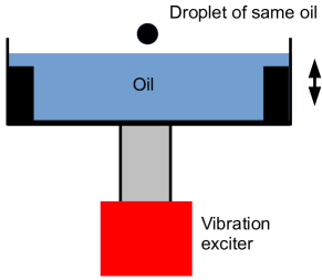
Figure 1: The experimental apparatus. The shape of the container reduces unwanted waves from the edge.

2 Basic mechanism

Figure 2: A droplet of silicone oil bouncing on the surface of the same liquid which is vibrated vertically. (courtesy Suzie Protière, Arezki Boudaoud and Yves Couder [5])

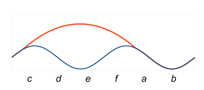
Figure 3: The height of the droplet (red) and the surface (blue) as it oscillates vertically with time. Surface waves are neglected. The labels cdefab refer to the photograph in figure 2.

To first order the height of the surface $h$ above the ambient level obeys the wave equation

$$\frac{1}{c^{2}}\frac{\partial^{2}h}{\partial t^{2}}~{}-~{}\frac{\partial^{2}h}{\partial x^{2}}~{}-~{}\frac{\partial^{2}h}{\partial y^{2}}~{}=~{}0$$ (1)

where $c$ is the wave speed. Figures 2 indicates that the waves are predominantly standing waves rather than propagating ones (note the reduced amplitude in photographs b and e). The relevant circularly symmetric solution is

$$h~{}~{}=~{}~{}-h_{o}~{}\cos(\omega_{o}t)~{}J_{o}(\omega_{o}\>r/c)$$ (2)

where $h_{o}$ is the maximum height and $J_{o}$ is a Bessel function of the first kind.

2.1 Parametric reinforcement

The standing waves in (2) are reinforced parametrically. See Figure 4. When the oil tray is at its greatest height it is accelerating downwards, typically at 3.3 – 4.3 g. This reverses the effective force of gravity, lifting the wave crests and enlarging the waves.

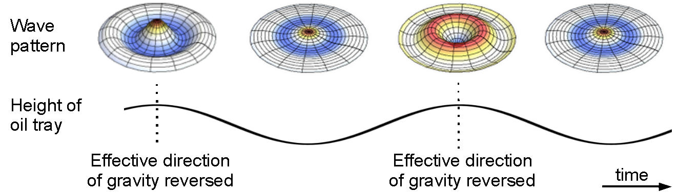
Figure 4: Parametric reinforcement of the standing waves in (2).

This can also be understood in terms of propagating waves as shown in figure 5. Like a pebble thrown into a pond, a droplet creates outgoing propagating waves when it lands. They are reinforced and reflected back when the oil tray is at its greatest height. The combination of outgoing and incoming waves forms the standing waves.

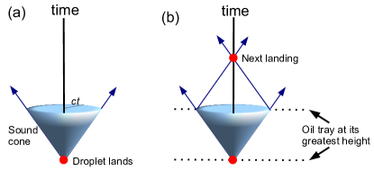
Figure 5: Bragg reflection. (a) When a droplet lands it creates a trough in the surface which propagates outwards (marked ‘sound cone’). (b) When the oil tray is at its greatest height it accelerates downwards. This reverses the effective direction of gravity, reinforcing the wave and forming an inward-directed trough that reaches the centre when the droplet next lands.

When the parametric driving is large enough, each bounce of the droplet influences the next through this mechanism. The system behaves as if it had a memory of previous bounces; this is called the ‘high memory’ regime.

2.2 Wave speed

The speed $c$ in (1) depends on frequency. We do not pursue this complication since the frequency was not varied in the experiments.

Consider an isolated propagating wave. If it oscillates in-phase with the forcing acceleration (similar to figure 4) at one position, it will have the opposite phase a quarter of a wavelength away. Thus, any effect on the wave speed will approximately cancel and the phase velocity is largely unaffected.

But the standing wave (2) near the droplet is always in-phase with the forcing acceleration. The restoring force on the wave is proportional to $h\{g-a_{m}\cos(2\omega_{o}t)\}$ where $a_{m}$ is the maximum vertical acceleration, so the net change of momentum on a half-cycle is proportional to

$$\int_{-\frac{\pi}{2}}^{\frac{\pi}{2}}\cos(\omega_{o}t)\{g-a_{m}\cos(2\omega_{o}t)\}dt\propto g-\frac{a_{m}}{3}$$

Since $a_{m}>3g$ in all the relevant experiments, the parametric driving outweighs the net restoring force of gravity and reverses it, leaving only surface tension to restore the waves. This substantially reduces the speed $c$. Surface tension is less effective in restoring larger waves, which are slowed the most. These standing waves are the ones that interact with the droplet and determine its motion, so we will need a reduced value of $c$ in the equations that follow.

If the forcing acceleration is increased further, eventually it overcomes the restoring force of surface tension and $c$ approaches zero, resulting in a Faraday instability [6].

3 Lorentz symmetry

The droplet in figure 2 moves to the right as it bounces. Its speed depends on the vertical driving acceleration as shown in Figure 6.

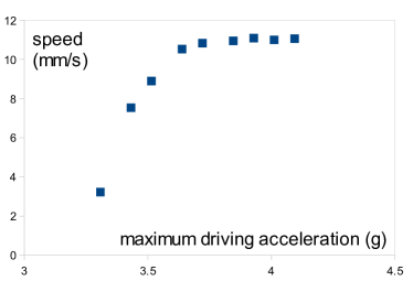
Figure 6: The speed of a walker depends on the maximum vertical driving acceleration, graphed as a multiple of the acceleration $g$ due to gravity. (Data courtesy Antonin Eddi, published in [7])

As we can see in figure 7, at low speed the droplet merely appears to be displaced slightly to the right, but as the parametric driving and the droplet speed increase, the wave field supporting the droplet becomes more complex. See Oza, Rosales and Bush for a detailed treatment [8].

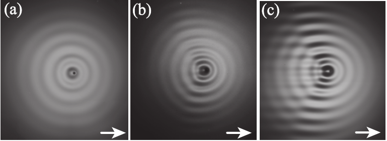
Figure 7: A droplet moving to the right. At low speed (left) it has been displaced from the centre; at higher speeds the wave field becomes more complex. (Courtesy Antonin Eddi, Eric Sultan, Julien Moukhtar, Emmanual Fort, Maurice Rossi and Yves Couder [7])

3.1 Simplified model

We now derive a simplified model of this motion using the symmetries of the wave equation, and test its predictions against the experimental data.

If $h(x,y,t)$ obeys the wave equation (1), then so does $h(x^{\prime},y^{\prime},t^{\prime})$ where

$$x^{\prime}~{}~{} =~{}~{}\gamma~{}(x-vt)$$

$$y^{\prime}~{}~{} =~{}~{}y$$

$$t^{\prime}~{}~{} =~{}~{}\gamma\left(t-\frac{vx}{c^{2}}\right)$$

$$\gamma~{}~{} =~{}~{}\frac{1}{\sqrt{1-\frac{v^{2}}{c^{2}}}}$$ (3)

This is the Lorentz transformation familiar from electromagnetism; it also applies to solutions of the wave equation in fluids, and is used in aerodynamics and acoustics (e.g. [9]). Applying it to (2) for the waves near a stationary droplet gives $\cos(\omega_{o}t^{\prime})J_{o}(\omega_{o}r^{\prime}/c)$ where $r^{\prime 2}=x^{\prime 2}+y^{\prime 2}$, which is illustrated in Figure 8.

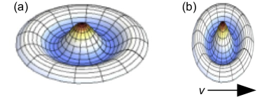
Figure 8: (a) The waves near a stationary droplet $\cos(\omega_{o}t)J_{o}(\omega_{o}r/c)$ (b) The Lorentz-boosted wave field $\cos(\omega_{o}t^{\prime})J_{o}(\omega_{o}r^{\prime}/c)$ moves at speed $v$.

In the moving solution, all lengths in the direction of travel have contracted by the factor $1/\gamma$ (substitute $t=0$ into (3)), while all time periods have dilated by the factor $\gamma$ (substitute $x=vt$).

The driving frequency is fixed, so the wave field of the droplet must adapt to compensate. If $h(x^{\prime},y^{\prime},t^{\prime})$ obeys the wave equation then so does $h(\alpha x^{\prime},\alpha y^{\prime},\alpha t^{\prime})$ where $\alpha$ is a scale factor. Choosing $\alpha=\gamma$ gives

$$x^{\prime\prime}~{}~{} =~{}~{}\gamma^{2}(x-vt)$$

$$y^{\prime\prime}~{}~{} =~{}~{}\gamma~{}y$$

$$t^{\prime\prime}~{}~{} =~{}~{}\gamma^{2}\left(t-\frac{vx}{c^{2}}\right)$$

Applying this coordinate transformation to (2) gives

$$h=-h_{o}\>\cos\left(\omega_{o}t-\frac{\gamma^{2}\omega_{o}v}{c^{2}}\Delta x\right)J_{o}\left(\frac{\omega_{o}}{c}r^{\prime\prime}\right)$$ (4)

where $\Delta x=x-vt$. This may be a reasonable approximation to the waves near a walker because it obeys the wave equation, it moves at speed $v$, and it bounces at constant frequency.

As the vertical acceleration increases, the droplet is thrown higher and lands later in the cycle (see figure 3). Suppose it lands at $t=n\tau+T$ where $\omega_{o}\tau=2\pi$. From (4) with $(\Delta x,y,t)=(0,0,T)$,

$$\frac{\partial h}{\partial x} =-h_{o}~{}\frac{\gamma^{2}\>\omega_{o}}{c}~{}\left(\frac{v}{c}\>\sin(\omega_{o}T)\right)$$

$$\frac{\partial^{2}h}{\partial x^{2}} =h_{o}~{}\frac{\gamma^{4}\>\omega_{o}^{2}}{c^{2}}\>\left(\frac{v^{2}}{c^{2}}\cos(\omega_{o}T)+\frac{1}{2}\right)$$ (5)

The sloping surface displaces the droplet from the centre, as we can see in figure 7. It will settle near $\partial h/\partial x=0$, where, from (5),

$$\gamma^{2}\omega_{o}\left(\frac{v^{2}}{c^{2}}+\frac{1}{2}\right)\>\Delta x~{}~{}=~{}~{}vT$$

where we have approximated $\sin(\omega_{o}T)=\omega_{o}T$ and $\cos(\omega_{o}T)=1$. Subsequent waves will always be generated at this displaced position, with the net result that the wave pattern moves at speed $v\propto\Delta x$ to first order, and

$$\gamma^{2}\left(\frac{v^{2}}{c^{2}}+\frac{1}{2}\right)~{}~{}\propto~{}~{}T$$ (6)

3.2 Comparison with experiment

The test for such a simplified model can only come from the experimental data, and we see in Figure 9 that the linear relationship we derive between $\gamma^{2}(v^{2}/c^{2}+\tfrac{1}{2})$ and $T/\tau$ is remarkably accurate out to an acoustic Lorentz factor of $\gamma=2.6$. The landing time $T$ was obtained from the intersection between the path of the droplet, for which $\ddot{h}=-g$, and the vertical oscillation of the oil tray (see figure 3 where the maximum acceleration was 3.5g). The characteristic speed $c$ of the standing waves near the droplet was taken to be $11.95$ mm/s, which is 8% larger than the maximum speed measured.

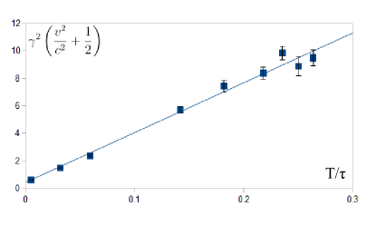
Figure 9: The experimental data in figure 6 plotted on new axes. $T$ is the landing time. Compare equation 6.

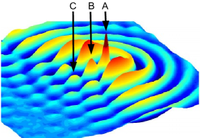
Figure 10: The wave field near a walker at large driving amplitude. Courtesy Antonin Eddi, Eric Sultan, Julien Moukhtar, Emmanual Fort, Maurice Rossi and Yves Couder [7]

There is further information in detailed velocimetry studies, reported by Eddi, Sultan, Moukhtar, Fort and Couder in [7]. Figure 10 is the wave field measured near a walker at high parametric driving. Successive bounces of the droplet can be seen in the peaks marked $A,B$ and $C$. We can obtain an approximation to the wave field by treating these three peaks as the centres of three wave fields given by (4). This is approximate because it neglects viscosity and nonlinearities such as those introduced by the parametric driving.

The three waves reinforce nearly perpendicular to the direction of motion, as can be seen from the taller waves there. They interfere destructively at an angle behind them, producing the wake-like lines with nearly zero amplitude.

Taller waves have a reduced wave speed, due to the parametric driving, which will compress the wave pattern perpendicular to the direction of motion. At the same time, the wave pattern is elongated parallel to the direction of travel because the source ($A,B,C$) is elongated. However, there is a counteracting effect. The Lorentz contraction in (4) compresses the wave pattern in the direction of motion. As we can see in figure 11, the resulting waves are roughly circular. See [7, 10] for further studies of the wave field.

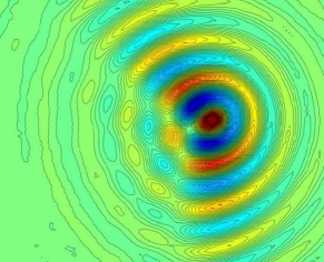
Figure 11: Contours of the waves in figure 10.

We conclude that bouncing droplets can be considered to be Lorentz covariant, to a good approximation, up to a Lorentz factor of 2.6.

We now turn to experiments conducted at constant forcing frequency and amplitude, where the velocity of the droplet is constant and the perturbations inflicted by the parametric driving on the Lorentz symmetry can largely be treated as constant and neglected.

4 Force between droplets

When a walker approaches the edge of the container, it does not actually touch the edge but is deflected away. The stroboscopic photograph in figure 12 shows a droplet travelling three times round a rectangular dish. This experiment gives deep insight into one type of interaction between droplets.

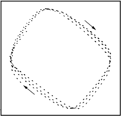
Figure 12: Stroboscopic photograph of a droplet’s path (dots) deflected near the walls of the container (solid). (Courtesy Suzie Protière, Arezki Badaoud and Yves Couder) [5]

4.1 Velocity normal to the boundary

The velocity normal to the boundary, $V_{\perp}$, can be measured from the photograph in figure 12, where an equal time passes between each stroboscopic image. Figure 13 plots $V_{\perp}^{2}$ as a function of the inverse distance $\frac{1}{r}$ from the boundary.

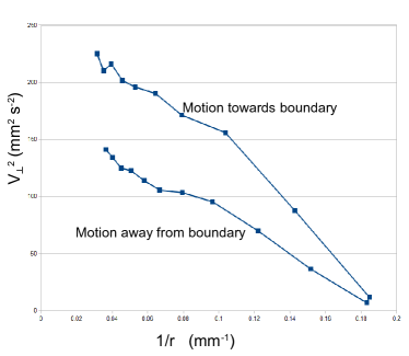
Figure 13: The square of the velocity normal to the boundary, $V_{\perp}^{2}$, as a function of inverse distance from the boundary. The data are extracted from the stroboscopic images near the bottom of figure 12.

For each branch in figure 13, the data near the boundary (towards the right of the graph) fall very nearly on a straight line, before deviating at greater distances. This straight line can be written

$$V_{\perp}^{2}~{}~{}=~{}~{}V_{o}^{2}~{}-~{}\frac{B}{r}$$ (7)

where the slope of the graph is $-B$ and it depends on the branch. Extrapolating to $1/r=0$ on the upper branch gives $V_{o}\approx~{}$18mm/s, which is the same as the speed of the droplet to the accuracy of measurement. The lower branch has $V_{o}\approx 14$mm/s.

4.2 Inverse square force

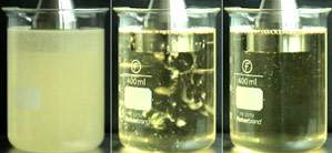
Figure 14: Degassing oil by applying ultrasonic vibration. The process takes about 5 seconds. (courtesy Hielscher Ultrasonics GmbH)

These experimental results show there is an inverse square force of repulsion near the boundary. The mechanism responsible for it is in fact well known [11]. It is used for removing unwanted bubbles of gas from oils and other liquids using ultrasonic vibration, as in figure 14. Ultrasonic pressure waves cause nearby bubbles to expand and contract in phase with one another, inducing oscillatory radial flows in the liquid. Near the mirror plane equidistant from two bubbles, the flows reinforce as illustrated in figure 15. The increased velocity results in a reduced Bernoulli pressure, giving rise to a force of attraction between the bubbles which merge and rise to the surface.

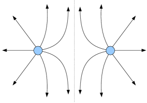
Figure 15: Schematic of the flow from two sources.

The exact same mechanism causes a bouncing droplet to avoid the boundary of the dish, which has the same effect as an imaginary image droplet on the other side, at the same distance, and bouncing antiphase. Each droplet drives radial flows in the liquid, just like those near the bubbles in the degasser – except that the bouncing droplets are antiphase, so the force is one of repulsion rather than attraction.

4.3 Size of the bubble force

In Figure 16, a vacuum cleaner nozzle ingests volume $Q_{1}$ of air per unit time. If the flow is spherically symmetric then the air speed at radius $r$ will be $U=-Q_{1}/(4\pi r^{2})$. A second nozzle at this radius, with volume $Q_{2}$ per unit time, will ingest momentum along with the air particles

$$\frac{dp}{dt}~{}=~{}\rho_{o}UQ_{2}~{}=~{}-\rho_{o}~{}\frac{Q_{1}Q_{2}}{4\pi r^{2}}$$ (8)

where $\rho_{o}$ is the density. This is an inverse square force of attraction between the nozzles.

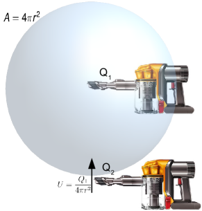
Figure 16: The flow near two vacuum cleaner nozzles, neglecting exhaust.

The direction of flow, and hence of the force, will be reversed if one of them is set to blow; then the force will be reversed for both hoses, by conservation of momentum (we assume the flow remains spherically symmetric, which might be achieved using a baffle on the end of the hose). More generally, oscillatory motion results in an attractive force if it is in-phase, and a repulsion if it is antiphase. The magnitude of the force is given by (8) averaged over a cycle.

4.4 Size of the droplet force

In the droplet experiments, the force in (8) must be doubled due to the hemispherical geometry but halved to average over a cycle, leaving its magnitude unchanged.

Suppose a droplet of volume $V$ bounces at frequency $f$. It will induce a flow $fV$ directly, which will be enhanced by secondary flows due to entrained fluid and the reinforced waves, giving $Q=\beta fV$ where $\beta$ is a factor into which we will also incorporate the effects of higher harmonics. Substituting into (8) and remembering to invert the sign, the acceleration of a droplet is

$$a~{}=~{}-\frac{F}{\rho_{o}V}~{}=~{}\frac{V\beta^{2}f^{2}}{4\pi r^{2}}$$

Using $f=25$Hz and a droplet radius of 0.35mm (which was reported for a different run), the acceleration measured in the upper branch of figure 13 gives $\beta\approx 5$.

4.5 Bubble force in conventional form

An inverse square force can always be written in the form

$$F~{}~{}=~{}~{}\alpha~{}\frac{\mathchar 22\relax\mkern-9.0mub\mkern 2.0muc}{r^{2}}$$ (9)

where $\alpha$ is a dimensionless constant and $\mathchar 22\relax\mkern-9.0mub\mkern 2.0mu$ is a constant with the dimensions of energy $\times$ time.

Suppose the radius of a bubble is given by

$$r_{b}~{}~{}=~{}~{}r_{o}(1+A\sin\omega t)$$

We will simplify the calculation by assuming that $A$ is small. The flow speed at the surface is

$$v_{s}~{}~{}=~{}~{}\frac{dr_{b}}{dt}~{}~{}=~{}~{}A~{}r_{o}\omega\cos(\omega t)$$

Multiplying by the area, the flow is $Q=4\pi r_{o}^{2}v_{s}$. Substituting into (8) gives

$$F~{}~{} =~{}~{}4\pi\rho_{o}r_{o}^{3}.r_{o}^{3}A^{2}\omega^{2}\cos^{2}(\omega t)\frac{1}{r^{2}}$$

$$=~{}~{}3m_{d}.r_{o}^{3}A^{2}\omega^{2}\frac{1}{2r^{2}}$$

where $m_{d}$ is the displaced mass of the bubble and we have replaced $\cos^{2}(\omega t)$ by its average value, $\frac{1}{2}$.

This can be rearranged into the conventional form (9) using the fact that the inertial mass of the bubble, due to the motion of the displaced fluid around it, is approximately $m=\frac{1}{2}m_{d}$ [11]. Thus

$$\alpha~{}~{} =~{}~{}3A^{2}~{}\left(\frac{r_{o}\omega}{c}\right)^{3}$$

$$\mathchar 22\relax\mkern-9.0mub\mkern 2.0mu~{}~{} =~{}~{}\frac{mc^{2}}{\omega}$$ (10)

The dimensionless constant $\alpha$ depends on whether the bubbles are resonant or not. Consider the resonant case. Neglecting geometric factors (which are of order 1), the bubble radius will vary from a small value to $2r_{o}$, giving $A\approx 1$. The maximum surface speed $r_{o}\omega$ will also increase, but it cannot much exceed the speed of sound in the fluid since the pressure would reduce to zero due to the Bernoulli effect. Therefore, if the bubbles are resonant then both $A$ and the ratio $r_{o}\omega_{o}/c$ will be of order 1, and so $\alpha$ is also of order 1.

4.6 Constant of the motion

If an unperturbed acoustic Lorentz transformation (3) could be realized experimentally, $\mathchar 22\relax\mkern-9.0mub\mkern 2.0mu$ would be a constant of the motion. The effective mass $m$ of a wave is proportional to its volume, so the Lorentz contraction multiplies it by $1/\gamma$, whilst the angular frequency is multiplied by the same factor, so $\mathchar 22\relax\mkern-9.0mub\mkern 2.0mu\propto m/\omega$ is independent of velocity. More formally, its dimensions, energy $\times$ time, are Lorentz invariant.

The droplet’s speed was not varied during the experiments. One way to achieve this might be to adjust the forcing amplitude and frequency (correcting for the perturbation to the wave speed and height). Alternatively a droplet of ferrofluid might be de-weighted magnetically so it lands later in the cycle and travels faster. The forcing frequency might be adjusted to avoid the additional factor $(1-v^{2}/c^{2})$ from the scale enlargement in (4). The mass of the droplet itself must be treated separately from that of the waves.

4.7 Comparison to the force between electrons

The electrostatic force between electrons is

$$F~{}~{} =~{}~{}\alpha~{}\frac{\hbar c}{r^{2}}$$

$$\alpha~{}~{} \approx~{}~{}\frac{1}{137.036}$$

$$\hbar~{}~{} =~{}~{}\frac{mc^{2}}{\omega}$$

where $m$ is the mass of the electron, $\omega$ its angular frequency, $c$ is the speed of light, and $\hbar$ = $h/2\pi$ where $h$ is Planck’s constant.

Notice the analogy to (9) and (10), where $\mathchar 22\relax\mkern-9.0mub\mkern 2.0mu$ is defined in the same way as $\hbar$.

From the value of $\alpha$, it seems that the electrostatic force is about two orders of magnitude weaker than the mechanical force between resonant bubbles. This suggests one limitation of the bouncing-droplet experiment as a model of quantum mechanics, namely that spherically-symmetric resonant solutions are not a good model for the electron. We will explore higher-order solutions that are not spherically symmetric below.

4.8 Maxwell’s equations

When the droplets or bubbles are stationary, we have seen there is an inverse square force between them (when averaged over a cycle). This obeys the same equations as the electrostatic field near a charged particle, since both are inverse square.

These equations can be extended to the case of moving droplets by noting that the solutions are acoustically Lorentz covariant to a reasonable approximation. So we need equations that are Lorentz covariant and that reduce to the equations of electrostatics when stationary.

These conditions are met by Maxwell’s equations with an acoustic value of $c$. In fact, they are unique in that Maxwell’s equations (more strictly, equations that are equivalent to them when they are averaged over a cycle) are the only ones that satisfy them. Suppose the contrary, that there existed a different set of Lorentz covariant equations that produce the same electric field with the same boundary conditions. The only difference between the two solutions can be in the magnetic field. But a Lorentz transformation turns a pure magnetic field into one with an electrical component, and so the electrical fields differ in the new reference frame. This is a contradiction. Thus the interaction between the droplets obeys Maxwell’s equations when it is averaged over a cycle.

This model predicts an interaction obeying the equations of magnetism, which is observed experimentally as follows.

4.9 Magnetic interaction

We now turn to the lower branch of figure 13.

A walker’s speed is fixed by the driving amplitude as discussed above. As the walker’s velocity normal to the boundary slows down and reverses in the experiment, it must accelerate parallel to the wall to maintain constant speed. The velocity boost is observed in the experiment. The researchers estimated the angle of incidence (relative to the normal to the boundary) at about $38^{\circ}$, and of reflection at about $53^{\circ}$.

In addition to the force of repulsion between the droplets, which obeys the same equations as those of electrostatics, there is a force of attraction when they are moving at a common velocity $v$ parallel to the boundary. This obeys the equations of magnetism. It is like the magnetic force of attraction between two electrons moving at a common velocity parallel to one another.

The magnetic force reduces the total force by a factor $1-v^{2}/c^{2}$, which accounts for the reduced slope of the lower graph in figure 13. We will take the approximation that the upper branch in figure 13 has no velocity perpendicular to the direction of travel, but by the time the droplet has reached the lower branch it has been accelerated to the full perpendicular speed, $v$ = 18 mm s^-1 by the tangential force. The force is proportional to the slope of the graph, whose ratio is 14/18. Equating these two gives $v=0.47c$, which suggests the droplets were moving at about half the wave speed.

4.10 Propagating waves

Maxwell’s equations tell us that if a source is accelerated, propagating waves will be emitted. We are not aware of attempts to test for these waves experimentally with droplets. This might be possible by accelerating droplets of a ferrofluid horizontally using magnetics. The period of the acceleration should be longer than that of the droplets.

We predict that propagating waves will be observed that are modulations of the standing waves surrounding the source (not ordinary longitudinal or transverse waves). They obey Maxwell’s equations with an acoustic value of $c$.

The force obeying Maxwell’s equations is only one of the interactions between droplets. To see another we must turn to coherent motion.

5 Diffraction

We saw how a droplet is repelled from a barrier. When the barrier has one or more slits in it, some droplets pass through as we can see in figure 17.

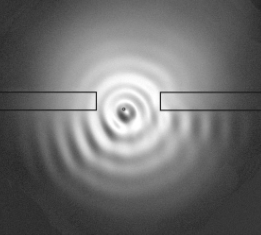
Figure 17: A droplet passing through an aperture in a submerged barrier.

When the Paris team measured which direction they went, they found classical diffraction patterns as you see for light waves, water waves or quantum mechanical particles, as in figure 18.

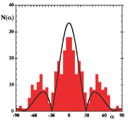
Figure 18: Histogram showing the number $N$ of droplets (out of 125) that emerge at angle $\alpha$ to the normal at large distance. The solid line is a single-slit diffraction pattern. Courtesy Yves Couder and Emmanuel Fort [12].

Diffraction is only observed in the high memory regime. In the low memory regime the waves from a droplet have little effect because they propagate away and are lost to viscosity.

In these experiments the forcing frequency and amplitude, and hence the walker velocity $|v|$, were kept constant. The variation was in $v_{x}$ and $v_{y}$.

5.1 Wavelength

We saw (equation 2) that the surface height near a stationary droplet has two component factors which we will now write $\psi$ and $\chi$ where

$$h~{}~{} =~{}~{}\psi~{}\chi$$

$$\psi~{}~{} =~{}~{}\cos(-\omega_{o}t)$$

$$\chi~{}~{} =~{}~{}~{}-h_{o}~{}J_{0}(k_{r}r)$$ (11)

We are interested in how the wave field of a moving droplet varies in the $x$ direction, neglecting $v_{y}$. An acoustic Lorentz transformation (3) gives the approximate solution

$$\psi~{}~{} =~{}~{}\cos(-\omega_{o}t^{\prime})$$

$$\chi~{}~{} =~{}~{}~{}-h_{o}~{}J_{0}(k_{r}r^{\prime})$$

where for simplicity we have neglected the scale enlargement in (4), which is just a constant since $|v|$ is constant. In this moving solution, the wave field $\chi$ advances with the droplet at speed $v_{x}$, and $\psi$ has become a planar wave which can be written

$$\psi~{}~{}=~{}~{}\cos(kx-\omega t)$$ (12)

The values of $k$ and $\omega$ can be obtained by defining $S=-\omega_{o}t^{\prime}$ and noting, from (3),

$$k~{}~{} =~{}~{}\frac{\partial S}{\partial x}~{}~{}=~{}~{}\frac{\partial S}{\partial t^{\prime}}\frac{\partial t^{\prime}}{\partial x}~{}~{}=~{}~{}\frac{\gamma\omega_{o}}{c^{2}}~{}v_{x}$$

$$\omega~{}~{} =-\frac{\partial S}{\partial t}~{}~{}=-\frac{\partial S}{\partial t^{\prime}}\frac{\partial t^{\prime}}{\partial t}~{}~{}=~{}~{}\gamma\omega_{o}$$ (13)

The wavelength of $\psi$ is $\lambda=2\pi/k$, or

$$\lambda~{}~{}=~{}~{}\frac{2\pi c^{2}}{\omega v_{x}}~{}~{}=~{}~{}\frac{b}{p}$$ (14)

where $p=mv_{x}$ is the momentum of the wave and $b=2\pi\mathchar 22\relax\mkern-9.0mub\mkern 2.0mu$ where $\mathchar 22\relax\mkern-9.0mub\mkern 2.0mu=mc^{2}/\omega$.

If we choose $m$ to be the effective mass of the wave (as discussed in section 4.6), then the parameter $\mathchar 22\relax\mkern-9.0mub\mkern 2.0mu$ that determines the wavelength of a droplet is the same as the constant in (10) that determines its deflection from the boundary by the inverse square force.

Equation (14) is the same as the de Broglie wavelength of a quantum mechanical particle with $b$ instead of Planck’s constant $h$. It can be extended to arbitrary axes. If the velocity in the direction of interest is ${\bf v}=(v_{x},v_{y})$ then $\psi$ in (12) becomes

$$\psi~{}~{}=~{}~{}\cos({\bf k}.{\bf x}-\omega t)$$ (15)

where

$${\bf p}~{}~{}=~{}~{}\mathchar 22\relax\mkern-9.0mub\mkern 2.0mu{\bf k}$$ (16)

and ${\bf p}=(p_{x},p_{y})$ is the momentum.

5.2 The diffraction pattern

We now show that the histogram in figure 18 agrees with the diffraction pattern of $\psi$ through the aperture.

The width of the aperture was 14.8 mm and, based on measuring the vertical distance from the barrier to the first node (measured near the corner to the right of the aperture), the wavelength of $\psi$ near the aperture was $\lambda=$ 7.3 mm. When waves of wavelength $\lambda$ diffract through a single aperture of width $L$, the first minimum of amplitude is at angle $\theta$ where $\lambda=L\sin\theta$. The above measurements predict this will occur at $\theta=30^{\circ}$. The minimum in the experimental histogram occurs between $30^{\circ}$ and $35^{\circ}$.

So we observe that the minimum in the histogram occurs where the waves of $\psi$ interfere destructively. It is as if the droplet were repelled from these regions. This can be understood as follows. Bigger waves have deeper wave troughs, so a droplet bouncing in them will be physically lower than one bouncing elsewhere. Consequently it will be attracted towards them by the force of gravity. Thus droplets move away from the regions of destructive interference of $\psi$ where the waves are smaller.

5.3 Double-slit diffraction

In another experiment, the droplet was made to diffract through two slits.

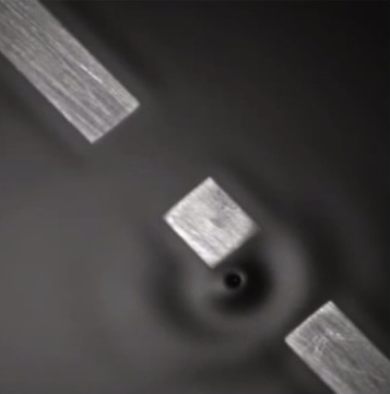
Figure 19: Droplet passing through a double slit

The histogram of the directions taken by the droplets after they had passed through one or other of the slits is shown in figure 20.

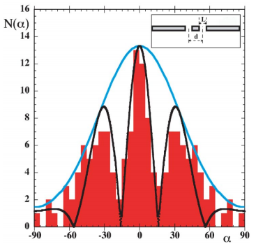
Figure 20: Histogram of the deflection angle for 75 droplets that have passed through one of two slits. The solid lines show a possible fit to a double-slit diffraction pattern. Courtesy Yves Couder and Emmanuel Fort [12].

The distance between the slits was 14.3mm. Using the above parameters we would expect the first diffraction minimum to be at approximately $15^{\circ}$, and this is what the researchers observed.

5.4 Classical approximation

Defining a quantity with the dimensions of energy

$$E~{}~{}=~{}~{}\mathchar 22\relax\mkern-9.0mub\mkern 2.0mu\omega$$

then, from (13),

$$\omega^{2}-c^{2}k^{2}~{}~{} =~{}~{}\omega_{o}^{2}$$

$$E^{2}-p^{2}c^{2}~{}~{} =~{}~{}m_{o}^{2}c^{4}$$

where we have used $p^{2}=\mathchar 22\relax\mkern-9.0mub\mkern 2.0mu^{2}k^{2}$ from (16) and the definition of $\mathchar 22\relax\mkern-9.0mub\mkern 2.0mu$ in (10). This will be recognised as the relativistic equation of motion for a classical particle of rest mass $m_{o}$ and energy $E$. It has a low-velocity approximation

$$E~{}~{}=~{}~{}E_{o}\left(1+\frac{p^{2}c^{2}}{E_{o}^{2}}\right)^{\frac{1}{2}}~{}~{}\approx~{}~{}E_{o}+\frac{p^{2}}{2m_{o}}$$

which is the Newtonian equation of motion.

In order to include the inverse square force discussed above, it suffices to add a term to the energy, namely

$$\mathchar 22\relax\mkern-9.0mub\mkern 2.0mu\omega~{}~{}=~{}~{}E~{}~{}=~{}~{}mc^{2}~{}-~{}V$$ (17)

where $V$ is the potential energy associated with the interaction.

Revisiting the experimental constraints, in principle it might be possible to adjust the forcing frequency in accordance with (17) during the experiment, but this was not done. The fixed forcing frequency constrained $|v|$ to be constant. As we saw in figure 12, the velocity perpendicular to the direction of interest will adjust to compensate. The experimenters observed an increased tangential speed when the droplets were near the diffraction slits, but the perturbation to the expected diffraction patterns, if any, was small.

5.5 Klein-Gordon equation

From (11), the factor $\psi$ for a stationary particle obeys the equation

$$\frac{\partial^{2}\psi}{\partial t^{2}}~{}~{}=~{}~{}-\omega_{o}^{2}\psi$$ (18)

In order to extend this to the case of a moving particle, we need a Lorentz covariant equation that reduces to (18) in the stationary case, namely

$$\frac{\partial^{2}\psi}{\partial t^{2}}~{}-~{}c^{2}\nabla^{2}\psi~{}~{}=~{}~{}\omega_{o}^{2}\psi$$ (19)

since the left hand side is Lorentz invariant.

Equation (19) is the same as the Klein-Gordon equation of quantum mechanics for a relativistic particle. The only difference is that the characteristic speed in the experiment is the speed of surface waves in the oil rather than the speed of light.

5.6 Schrödinger equation

If (11) receives a Lorentz boost with a small velocity $v$ in the $x$ direction then we get $\psi=\cos(-\omega_{o}t^{\prime})=\cos(vx\omega_{o}/c^{2}-\omega_{o}t)$ where we have approximated $\gamma=1$. Writing this in the form

$$\psi~{}~{}=~{}~{}R\cos(\theta-\omega_{o}t)$$ (20)

gives $\theta=vx\omega_{o}/c^{2}$. Extending to arbitrary axes gives the velocity of the droplet as determined by the local waves

$${\bf v}~{}~{}=~{}~{}\frac{c^{2}}{\omega_{o}}\>\nabla\theta$$ (21)

The function in (20) can be analytically continued into the complex plane by defining

$$\psi_{s}~{}~{}=~{}~{}R\>e^{i\theta}$$ (22)

so that $\psi=\Re(e^{-i\omega_{o}t}\psi_{s})$ where $\Re$ means the real part. Now, $\psi$ obeys the Klein-Gordon equation (19), and we will seek a solution where both the real and imaginary parts of $e^{-i\omega_{o}t}\psi_{s}$ obey this same equation, which is satisfied when

$$i\>\frac{\partial\psi_{s}}{\partial t}~{}~{}=~{}~{}-\frac{c^{2}}{2\omega_{o}}\>\nabla^{2}\psi_{s}$$ (23)

where we have neglected the term in $\partial^{2}\psi_{s}/\partial t^{2}$, which is small when the velocity is small.

Substituting (17) in the form $\mathchar 22\relax\mkern-9.0mub\mkern 2.0mu\omega_{o}=m_{o}c^{2}-V$ gives

$$i\>\mathchar 22\relax\mkern-9.0mub\mkern 2.0mu\>\frac{\partial\psi_{s}}{\partial t}~{}~{}=~{}~{}\left(-\frac{\mathchar 22\relax\mkern-9.0mub\mkern 2.0mu^{2}}{2m_{o}}\nabla^{2}+V\right)\psi_{s}$$ (24)

This is the same as the Schrödinger equation for the wavefunction of a quantum mechanical particle. The only difference is that the constant of motion in the experiment is $\mathchar 22\relax\mkern-9.0mub\mkern 2.0mu$ rather than Planck’s reduced constant $\hbar$ (although they are defined in the same way and they are both constants of the motion).

5.7 Probability density

If the starting position of a droplet is not known precisely, and it is allowed to evolve over time, then there will be a range of final positions, which can be calculated probabilistically. Our treatment will follow the reasoning of David Bohm [13], who solved this problem in 1952.

Substituting the definition $\psi_{s}=Re^{i\theta}$ (equation 22) back into (23), and taking the imaginary part when $\theta=0$ gives

$$\frac{\partial R}{\partial t}~{}~{}=~{}~{}-\frac{c^{2}}{2\omega_{o}}~{}(R\>\nabla^{2}\theta-2\>\nabla R\>\nabla\theta)$$

which can be rearranged into

$$\frac{\partial R^{2}}{\partial t}~{}+~{}\nabla(R^{2}~{}{\bf v})~{}~{}=~{}~{}0$$ (25)

where v is the velocity of the droplet in (21).

This equation has a simple interpretation. When the velocity ${\bf v}$ of a compressible fluid, such as the air, varies with position, its density $\rho$ obeys the continuity equation $\frac{\partial\rho}{\partial t}+\nabla(\rho~{}{\bf v})=0$, which is the same as (25) with $R^{2}$ replaced by $\rho$. Since the velocity of the droplets is v, it follows that the probability density for the position of the droplet, averaged over nearby trajectories, must be $R^{2}=|\psi_{s}|^{2}$ (provided the initial value of $|\psi_{s}|^{2}$ is appropriately calibrated, or ‘normalised’). This is confirmed by the experimental results in figure 21. The graph shows that the probability a droplet crosses the barrier (or ‘tunnels’) reduces exponentially with its width. If you solve Schrödinger’s equation with a barrier, you get the same exponential decay of $|\psi^{2}|$ with the width of the barrier. The same probability density $|\psi_{s}^{2}|$ is assumed as a postulate in the Copenhagen interpretation of quantum mechanics.

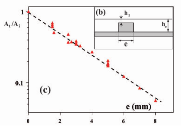
Figure 21: Droplets encounter a region of reduced depth, which repels them. The $x$ axis is the width of the barrier, and the $y$ axis is the probability the droplet tunnels through the barrier, plotted on a logarithmic scale. Courtesy Antonin Eddi [14]

The foregoing calculation was performed in 1952, more than 50 years before the first droplet experiments. It led Bohm to hypothesise the existence of a tiny particle which moves at the velocity v in (21), guided by waves that obey Schrödinger’s equation (23), whose probability density is $|\psi_{s}^{2}|$. These are exactly the equations for a bouncing droplet at low velocity. His insight is remarkable. For him, this was a purely abstract exercise; he did not have the droplet model to inspire him to derive these relationships from Euler’s equation.

Based on these equations, Bohm showed the resulting mechanics to be indistinguishable from the Copenhagen interpretation of quantum mechanics. He subsequently found that Louis de Broglie had suggested a similar idea in the 1920s; the model is now called the de Broglie-Bohm interpretation of quantum mechanics.

5.8 Same equations, same solutions

Given that we have the same mathematics up to a constant factor, we expect the calculations of quantum mechanics to carry over to other droplet experiments, and can start to understand why bouncing droplets are a pretty good model of the quantum world.

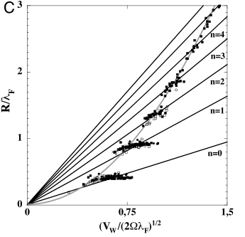
Figure 22: A droplet in a rotating bath is attracted towards the centre, and exhibits quantized orbits. Courtesy Emmanual Fort [15]

In figure 22, the experiment was conducted in a rotating bath, where the droplet was attracted towards the centre. The droplets exhibited quantized orbits.

Other experimentalists have discovered further evocative results. For example, Valeriy Sbitnev has recently reported that a droplet and an antidroplet (a bubble) can be created when two suitably-shaped soliton waves collide on the surface of the fluid [16]. The droplet and antidroplet move apart, just as when a particle and antiparticle are created in quantum mechanics. However, before we approach the domain of field theory, we first have to discuss spin.

6 Rotational motion

We have so far only considered waves with circular and spherical symmetry. The photographs in figure 23 suggest we also have to think about solutions to the wave equation which depend on angle.

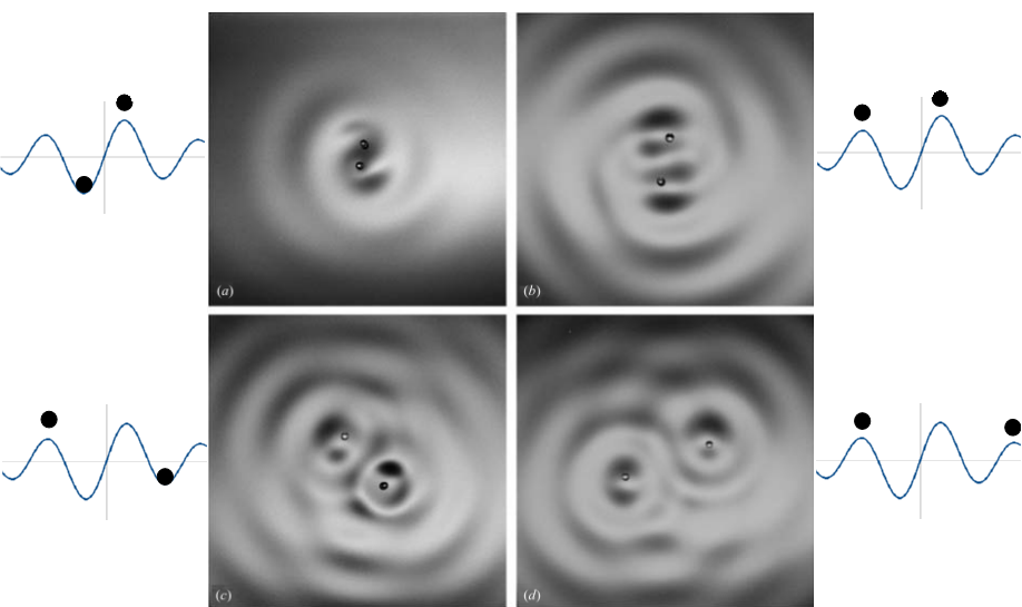
Figure 23: The waves with two droplets. The side drawings show a Bessel function $J_{1}$, which is the lowest rotating component of the standing waves between the droplets. The bouncing is antiphase in (a) and (c) and in sympathy in (b) and (d). (Photograph courtesy Suzie Protière, Arezki Boudaoud and Yves Couder [5])

In this experiment, the droplets orbit around one another with a period of approximately 20 bouncing periods in (a), and longer in (b)-(d). Their velocity is approximately that of an ordinary walker driven with the same vertical acceleration, and the period increases with radius.

6.1 Harmonic solutions

The motion in the photographs can be described using the solutions to the wave equation in circular coordinates $(r,\theta)$, namely

$$h_{m}~{}~{}=~{}~{}h_{o}~{}\cos(\omega_{o}t-m\theta)~{}J_{m}(k_{r}r)$$ (26)

where $J_{m}$ is a cylindrical Bessel function of the first kind, $m$ is an integer whose sign is significant, and $\omega_{o}=c~{}k_{r}$. The waves near the two droplets contain components with various values of $m$, but the main experimental results can be understood from the lowest order rotating components, with $m=\pm 1$. We neglect higher harmonics as well as $J_{o}$ in (b) and (d).

Figure 23 shows the Bessel function $J_{1}$, which gives the wave height of the lowest rotating component on a line joining the droplets. As we have seen, the droplets prefer to land in the wave troughs, so they are in free flight over the crests, as shown. The rotating wave pattern is

$$h~{}~{}= ~{}~{}\tfrac{1}{2}h_{0}\>[\cos(\omega_{o}t+\Omega t-\theta)~{}J_{1}(k_{1}r)$$

$$+~{}\cos(\omega_{o}t-\Omega t+\theta)~{}J_{1}(k_{2}r)]$$

$$\approx ~{}~{}h_{o}\>\cos(\omega_{o}t)~{}\cos(\Omega~{}t-\theta)~{}J_{1}(k_{r}r)$$ (27)

where $ck_{1}=\omega_{o}+\Omega$ and $ck_{2}=\omega_{o}-\Omega$. In the second expression we have used the identity $\cos(A+B)+\cos(A-B)=2\cos A\cos B$, and have approximated $k_{1}\approx k_{2}\approx k_{r}$, which is valid at small $r$ and $\Omega$. This can be regarded as a standing wave that rotates with the droplets at angular frequency $\Omega$.

The factor $\cos(\Omega t-\theta)$ vanishes on the node line $\theta=\Omega t\pm\frac{1}{2}\pi$. On either side of this line, its sign reverses; we see in the photographs in figure 23(b) – (d) that the crests turn into troughs and the troughs crests. The node line is nearly normal to the line joining the droplets, indicating that they are bouncing close to the angle with the largest wave amplitude. The pattern is not so evident in (a), due to the greater angular velocity and the presence of higher-order components.

6.2 Angular momentum

Figure 24 shows how the wave height $h_{1}$ in (26) varies with angle. The wave propagates in the $+\theta$ direction. The flow velocity u is irrotational ($\oint{\bf u.dl}=0$) when the path of integration dl is on the submerged line $A$, but this does not mean the wave has no angular momentum since it is not irrotational at $B$. The elevations carry extra fluid around the centre.

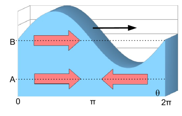
Figure 24: The wave $h_{1}$ in (26) at fixed radius at the instant $\omega_{o}t=\pi/2$. The flow speed (red arrows) is proportional to the wave height.

At large radius, the net flow around the centre approximates to that of a vortex when averaged over a period and a wavelength. The Bessel function in (26) approximates to a standing wave in the radial direction, whose amplitude reduces as $A\sim r^{-\frac{1}{2}}$. The flow speed is $u\propto A$ so the net flow is proportional to $uA\sim r^{-1}$, which is the same as a vortex.

At small radius the flow diverges from that of a vortex, and in particular there is no singularity. It is illustrated in figure 25.

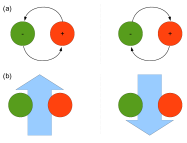
Figure 25: (a) Schematic drawing of the rotating droplet pair photographed in figure 23(a), and its image in the boundary. At the instant drawn, the green circles are the wave troughs (where the droplet lands) and the red circles are crests. (b) The fluid flow due to the rotational motion. The trough has negative volume and contributes to the flow in the same Cartesian direction as the crest.

6.3 Attraction to the boundary

Two vortices of opposite circulations are attracted towards one another because their flows reinforce in the region between them, giving a reduced Bernoulli pressure. The rotating pairs should similarly be attracted towards their images in the boundary, which rotate in the opposite direction. A protrusion on the boundary might be used to test for this.

The fine structure constant of the interaction is as follows. We saw that individual droplets are repelled from the boundary by an inverse square force. This static force obeys the equations of electrostatics, with a fine structure constant of $\alpha\sim 0.3$. We also saw evidence for a motion-dependent force which obeys the same equations as magnetism, in which a droplet and its image in the boundary are attracted towards one another when they both move in the same direction parallel to the boundary.

The static forces between a pair and its image in the boundary nearly cancel out, since if one droplet of a pair is attracted to the image then the other, being antiphase, will be repelled. However, the motion-dependent force is always attractive. For example, consider the interactions with the wave crest marked in red on the left of figure 25. It is moving in the same direction as the (green) trough in the image, an alignment which we saw produces a force of attraction (section 4.9). The crest in the image (red) moves in the opposite direction and with the opposite phase. Each of these individually reverses the direction of the interaction, so the combination leaves the sign unchanged.

We saw that the ratio of the moving to the static forces is $v^{2}/c^{2}$ (the same as the ratio of the magnetic to the electrostatic forces for particles moving at velocity $v$). The force on each droplet is doubled, since there are two images, but it must be averaged over a rotation, giving a factor of $\frac{1}{2}$. The fine structure constant of the interaction is thus

$$\alpha_{2}~{}~{}=~{}~{}\frac{v^{2}}{c^{2}}\>\alpha_{1}$$ (28)

where $\alpha_{1}$ is the fine structure constant for the static force between individual droplets. The strength of the interaction depends on the rotational speed, which can be varied in the experiment. A typical value might be $v=\frac{1}{4}c$ and $\alpha_{1}\sim 0.3$ giving $\alpha_{2}\sim 1/50$.

Our model predicts that an orbiting droplet pair will be attracted towards the boundary with this reduced fine structure constant. This phenomenon has been noted by the experimenters; orbiting pairs that approach a submerged boundary at a shallow angle can stick to it and then move along it, playing ‘hopscotch’ as each droplet takes it in turn to leapfrog the one in front. However an experiment with precise measurements has not yet been performed.

6.4 The emergence of spin-half behaviour

The rotating waves in (26) can be treated as independent because they are orthogonal in the sense that

$$\int_{0}^{2\pi}h_{m}~{}h_{n}~{}d\theta~{}~{} =~{}~{}0 (m\neq n)$$ (29)

as may be verified by direct substitution.

We have seen that the angular momentum of the wave $h_{1}$ in (23) is in the $+z$ direction (vertically upwards), and it is in the $-z$ direction for $h_{-1}$. The photograph in figure 23 shows the case where the waves have nearly equal amplitude. What if the amplitudes are not equal?

It simplifies the analysis to consider ‘degenerate’ solutions, that is, solutions that have the same energy. (Solutions of arbitrary energy can be obtained by scaling the wave height.) The degenerate solutions are

$$h~{}~{}=~{}~{}\cos(\alpha)\>h_{1}~{}+~{}\sin(\alpha)\>h_{-1}$$ (30)

where $\alpha$ is a real parameter. This is a solution to the wave equation because it is a sum of solutions. Its energy is proportional to $\cos^{2}\alpha+\sin^{2}\alpha$, which is constant, so the waves are degenerate. The angular momentum is

$$L~{}~{} =~{}~{}L_{o}(\cos^{2}\alpha-\sin^{2}\alpha)$$

$$=~{}~{}L_{o}\cos(2\alpha)$$ (31)

where $L_{o}$ is the angular momentum of $h_{1}$. The angular momentum and the wave pattern $h$ vary continuously with the parameter $\alpha$, as shown in the table below

$\alpha$	$L/L_{o}$	h
0	1	$h_{1}$
$\frac{\pi}{4}$	0	$\frac{1}{\sqrt{2}}(h_{-1}+h_{1})$
$\frac{\pi}{2}$	-1	$h_{-1}$
$\frac{3\pi}{4}$	0	$\frac{1}{\sqrt{2}}(h_{-1}-h_{1})$
$\pi$	1	$-h_{1}$

As we can see in the table, the wave field reverses sign after the direction of the angular momentum has gone through a complete cycle. Two cycles are needed to return to the starting position.

Fermions are like these waves, in that their wavefunctions reverse sign if the direction of their angular momentum is rotated through $360^{\circ}$. It is commonly believed that this behaviour cannot emerge from classical mechanics. However the rotating droplets show that this belief is wrong.

In fact, double symmetry is already known in systems that contain two harmonic sub-systems. Leroy, Bacri, Hocquet and Devaud provided another example in 2006 when they showed that two weakly coupled pendula with nearly the same frequency also have this symmetry [17].

6.5 Bloch sphere

The elementary waves in (26) are the real part of

$$\xi_{m}~{}~{}=~{}~{}A~{}e^{-i(\omega_{o}t-m\theta)}~{}J_{m}(k_{r}r)$$ (32)

where $A$ is the amplitude. This can be factored as before into

$$\xi~{}~{} =~{}~{}\psi\>\chi$$

$$\psi~{}~{} =~{}~{}e^{-i\omega_{o}t}$$

$$\chi~{}~{} =~{}~{}A~{}e^{im\theta}~{}J_{m}(k_{r}r)$$ (33)

The last section showed that $\psi$ obeys Schrödinger’s equation. Now let us examine the factor $\chi$.

When the wave height in (30) is extended into the complex plane as in (33), we get a simple way to provide an arbitrary origin of time for each of the two components

$$\chi=e^{iS}\left[\cos\left(\tfrac{1}{2}{\beta}\right)\chi_{1}+e^{i\varphi}~{}\sin\left(\tfrac{1}{2}\beta\right)\chi_{-1}\right]$$ (34)

where $S$ is an arbitrary overall phase, $\varphi$ is the relative phase of the two components, and we have defined $\beta=2\alpha$.

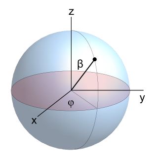
Figure 26: A Bloch sphere.

The parameters in this equation can be represented on a sphere as shown in figure 26. The angular momentum normal to the surface (in the z direction) is proportional to $\cos\beta$. When $\beta=\frac{1}{2}\pi$, the angular momentum vanishes and there are standing waves whose amplitude is greatest at angle $\varphi$ to the $x$ axis. However, this diagram should not be over-interpreted. It would be wrong to conclude that the system is physically oriented in the direction indicated in the figure. The existence of a simple geometrical way to picture the parameters in (34) should not blind us to the fact that we are describing ordinary surface waves which cannot rotate out of the plane of the surface.

Nonetheless, equation (34) is the same as that of a spin-half particle whose wavefunction is $\chi$ where $\chi_{1}$ is the spin-up state and $\chi_{-1}$ the spin-down state, which is usually represented on the ‘Bloch sphere’ in figure 26. By inspection, the sign of $\chi$ reverses when $\beta$ increases by $2\pi$, which is characteristic of spin-half systems.

6.6 Pauli spin matrices

The mapping of the wave height near a droplet onto the Bloch sphere can be shown more formally by writing (34) as a dot product of two vectors a and $\boldsymbol{\chi}$

$$\chi~{}~{}=~{}~{}{\bf a}.\boldsymbol{\chi}~{}~{}=~{}~{}(a_{1},a_{2}).(\chi_{1},\chi_{-1})$$

where the values of $a_{i}$ are obtained from (34). The angular momentum of the first component is proportional to $|a_{1}|^{2}$, and that of the second component is proportional to $-|a_{2}|^{2}$, so the normalised total is

$$\sigma_{z}~{}~{}=~{}~{}\frac{|a_{1}|^{2}-|a_{2}|^{2}}{|a_{1}|^{2}+|a_{2}|^{2}}$$ (35)

This can also be written

$$\sigma_{z}~{}~{}=~{}~{}\frac{{\bf a}^{*}.~{}\widehat{\sigma}_{z}\>{\bf a}}{{\bf a}^{*}.{\bf a}}$$ (36)

where $\widehat{\sigma}_{z}=(\begin{smallmatrix}1&0\\ 0&-1\end{smallmatrix})$ is the same as the Pauli spin matrix for the $z$ direction.

As in quantum mechanics, we can extend this as follows. The Pauli matrices are
$\widehat{\sigma}_{x}=(\begin{smallmatrix}0&1\\ 1&0\end{smallmatrix})$,  $\widehat{\sigma}_{y}=(\begin{smallmatrix}0&-i\\ i&0\end{smallmatrix})$,  $\widehat{\sigma}_{z}=(\begin{smallmatrix}1&0\\ 0&-1\end{smallmatrix})$, and spin projections $\sigma_{i}$ are defined by

$$\sigma_{i}~{}~{}=~{}~{}\frac{{\bf a}^{*}.~{}\widehat{\sigma}_{i}\>{\bf a}}{{\bf a}^{*}.{\bf a}}$$

where $i$ can be $x,y$ or $z$. The eigenvectors of $\widehat{\sigma}_{i}$ are

$\beta$	$\varphi$	$(a_{1},a_{2})$	$(\sigma_{x},\sigma_{y},\sigma_{z})$	Eigenvector of
$\frac{1}{2}\pi$	$0$	$\frac{1}{\sqrt{2}}(1,1)$	$(1,0,0)$	$\widehat{\sigma}_{x}$
$\frac{1}{2}\pi$	$\frac{1}{2}\pi$	$\frac{1}{\sqrt{2}}(-i,i)$	$(0,1,0)$	$\widehat{\sigma}_{y}$
$0$	$0$	$(1,0)$	$(0,0,1)$	$\widehat{\sigma}_{z}$

It will be noticed that $(\sigma_{x},\sigma_{y},\sigma_{z})$ correspond to the Cartesian coordinates of a unit vector at the spherical angle $(\beta,\varphi)$ in figure 26. This is the basis of the Bloch sphere, which maps between the two representations. The mapping is a double covering because $\chi$ reverses sign when $\beta$ increases by $2\pi$. The same mathematics is used to describe fermions in quantum mechanics.

6.7 Antisymmetry

When the driving amplitude is reduced, the rotation speed of the droplets photographed in figure 23 slows to zero. Figure 27 is a schematic of two droplet pairs near each other. $A$ is a solution to (34) with $(\beta,\varphi)=(\frac{1}{2}\pi,0)$ and $B$ has $(\frac{1}{2}\pi,\frac{1}{2}\pi)$.

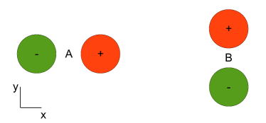
Figure 27: Schematic of two droplet pairs near each other. Elevations are marked red and depressions green.

The droplets in $B$ have opposite phases, so one will attract the other pair whilst the other repels and the net forces cancel. However, there is still an effect involving orientation. One droplet in $A$ is closer to $B$ than the other, which will cause $B$ to rotate anticlockwise. This prediction might be tested experimentally.

After $B$ has rotated into the preferred alignment, the solutions will be oriented in the $x$ direction and the wave height is the real part of

$$\xi~{}~{}=~{}~{}\xi_{a}({\bf x},t)~{}-~{}\xi_{a}({\bf x-d},t)$$ (37)

where $\xi_{a}$ is the wave due to $A$ and $\bf d$ is the separation of the pair, $B-A$.

Equation (37) is antisymmetric, and, in particular, exchanging $A$ and $B$ reverses the sign of the wave field. This may be compared to the principle, formulated by Wolfgang Pauli in 1925, that the total wave function for two identical fermions is anti-symmetric with respect to exchange of the particles.

7 Discussion

In this paper we have explained why the bouncing droplet experiments of Couder, Fort and colleagues are a pretty good model for quantum mechanics.

We have derived from first principles that bouncing droplets are, to a rather good approximation, Lorentz covariant, with $c$ being the speed of surface waves; that they obey an analogue of Schrödinger’s equation where Planck’s constant is replaced by an appropriate constant of the motion; that the force between them obeys Maxwell’s equations, with an inverse-square attraction and an analogue of the magnetic force; and finally that orbiting droplet pairs exhibit spin-half symmetry and align antisymmetrically as in the Pauli exclusion principle.

These results explain why droplets undergo single-slit and double-slit diffraction, tunnelling, Anderson localisation, and other behaviour normally associated with quantum mechanical systems. We make testable predictions for the behaviour of droplets near boundary intrusions, and for an analogue of polarised light.

The mathematical model described here may be useful as a teaching aid. Bouncing-droplet experiments have become popular with undergraduates; we show here that they can be explained with the mathematics routinely taught in a first undergraduate course in fluid mechanics. Indeed they are already sometimes one of the examples used to motivate such courses.

For an introductory course in quantum mechanics, droplet models might help students overcome the initial feeling of bewilderment at the quantum-mechanical wavefunction $\psi$. Here, $\psi$ emerges naturally from known physical principles. This should help explain how the wavefunction of several interacting particles can emerge as a function of their position, momentum and spin, yet still be defined as a single amplitude and a single phase at each point in space – helping students to avoid confusion over such concepts as configuration space and quantum entanglement. A vivid experimental model with a clear mathematical explanation should also help demystify spin-half behaviour and antisymmetry.

Finally, one might ask whether it is possible to extend this model from two dimensions to three. In separate work we show a model of rotons in liquid helium with similar properties to the droplets described here. Second sound in helium can be modelled as waves in a gas of quasiparticles, the lambda point as its Kosterlitz-Thouless transition, while transverse sound emerges as the polarised-light analogue whose existence we predict here for droplet experiments [18]. So there may be room for further research on even more complex and realistic analogue models of quantum mechanics.

References

- [1] J. Walker. Drops of liquid can be made to float on the liquid. What enables them to do so? Sci. Am, 238(6):123–129, 1978.
- [2] Y. Couder, S. Protière, E. Fort, and A. Boudaoud. Dynamical phenomena: Walking and orbiting droplets. Nature, 437(7056):208–208, 2005.
- [3] J. Moláček and J. W. M. Bush. Drops bouncing on a vibrating bath. Submitted to J. Fluid Mech., 2013.
- [4] Y. Couder. television programme. https://www.youtube.com/watch?v=W9yWv5dqSKk#t=14, cited January 2014.
- [5] S. Protière, A. Boudaoud, and Y. Couder. Particle-wave association on a fluid interface. Journal of Fluid Mechanics, 554(10):85–108, 2006.
- [6] T. B. Benjamin and F. Ursell. The stability of the plane free surface of a liquid in vertical periodic motion. Proc. Roy. Soc. London. A., 225(1163):505–515, 1954.
- [7] A. Eddi, E. Sultan, J. Moukhtar, E. Fort, M. Rossi, and Y. Couder. Information stored in faraday waves: the origin of a path memory. Journal of Fluid Mechanics, 674:433, 2011.
- [8] A. U. Oza, R. R. Rosales, and J. W. M. Bush. A trajectory equation for walking droplets: hydrodynamic pilot-wave theory. Journal of Fluid Mechanics, 737:552–570, 2013.
- [9] F. Dubois, E. Duceau, F. Maréchal, and I. Terrasse. Lorentz transform and staggered finite differences for advective acoustics. arXiv:1105.1485v1, 2011.
- [10] J. Moláček and J. W. M. Bush. Drops walking on a vibrating bath: towards a hydrodynamic pilot-wave theory. Submitted to J. Fluid Mech., 2013.
- [11] T. E. Faber. Fluid dynamics for physicists. Cambridge University press, Cambridge, UK, 1995.
- [12] Y. Couder and E. Fort. Single-particle diffraction and interference at a macroscopic scale. Phy. Rev. Lett., 97(15):154101, 2006.
- [13] D. Bohm. A suggested interpretation of the quantum theory in terms of ‘hidden’ variables. Physical Review, 85(2):166, 1952.
- [14] A. Eddi, E. Fort, F. Moisy, and Y. Couder. Unpredictable tunneling of a classical wave-particle association. Physical review letters, 102(24):240401, 2009.
- [15] E. Fort, A. Eddi, A. Boudaoud, J. Moukhtar, and Y. Couder. Path-memory induced quantization of classical orbits. Proceedings of the National Academy of Sciences, 107(41):17515–17520, 2010.
- [16] V. I. Sbitnev. Droplets moving on a fluid surface: interference pattern from two slits. arXiv:1307.6920v1, 2013.
- [17] V. Leroy, J. C. Bacri, T. Hocquet, and M. Devaud. Simulating a one-half spin with two coupled pendula: the free larmor precession. European journal of Physics, 27(6):1363, 2006.
- [18] R. Brady and R. Anderson. Emergent Quantum Mechanics. In preparation, 2014.