Numerical simulation of oscillating magnetospheres with resistive electrodynamics

Abstract

We present a model of the magnetosphere around an oscillating neutron star. The electromagnetic fields are numerically solved by modeling electric charge and current induced by the stellar torsional mode, with particular emphasis on outgoing radiation passing through the magnetosphere. The current is modeled using Ohm’s law, whereby an increase in conductivity results in an increase in the induced current. As a result, the fields are drastically modified, and energy flux is thereby enhanced. This behavior is however localized in the vicinity of the surface since the induced current disappears outwardly in our model, in which the exterior is assumed to gradually approach a vacuum.

1 Introduction

Giant flares in Soft Gamma-ray Repeaters (SGRs) are some of the most energetic astrophysical events. The total energy released during a flare is $\sim 10^{46}$ ergs, and flares are considered to be powered by a global reconfiguration of magnetic field $>10^{14}$ G in a magnetar (Mereghetti (2008) for a review). Global seismic oscillations of the stellar crust are likely to be associated with flares(Duncan, 1998). Quasi-Periodic Oscillations (QPOs) are observed in the decaying tails of the flares of SGR 1900+14 and SGR 1806-20, and their frequencies are in the range of 10-$10^{3}$ Hz, which are interpreted as the frequencies of torsional oscillations with some harmonic numbers (e.g., Israel et al. (2005); Strohmayer & Watts (2006)). The typical frequency of the torsional shear mode is $\sim 10$Hz, which is estimated from the shear modulus, density at the crust and stellar radius. More realistic treatment is necessary for the actual fitting. In particular, considering the effects of strong magnetic fields, which couple core and crust, is essential. A number of researchers have been exploring the oscillations of strongly magnetized stars (Piro (2005); Levin (2007); Lee (2008); Sotani et al. (2008); Cerdá-Durán et al. (2009); Colaiuda & Kokkotas (2011); van Hoven & Levin (2012); Gabler et al. (2012) and references therein).

In spite of substantial improvements in oscillation theory, there is considerable uncertainty about the processes behind X- and gamma-ray radiation phenomena. Main peaks in the power spectrum may correspond to the oscillation frequency, but their amplitudes and decays should be affected by the surrounding magnetosphere. Timokhin et al. (2000) showed that an oscillating magnetized star should have a magnetosphere filled with charge-separated plasma so that the longitudinal electric field (parallel to the magnetic field) in vacuum is screened. This situation resembles that of a pulsar magnetosphere. Rotation in pulsars is replaced by oscillation in magnetized stars. The induced charge density has been calculated as a generalization of the well-known Goldreich-Julian density for pulsars (Goldreich & Julian, 1969). In the almost analytic treatment in Timokhin et al. (2000), the current is assumed to be zero everywhere. In magnetar flares, large current associated with a magnetic twist $\vec{\nabla}\times\vec{B}\neq 0$ is expected to flow out from the surface. Therefore, it is necessary to consider the effects of flowing current on the magnetosphere. The calculations necessary to consistently determine the charge and current densities induced by the oscillation are more complex, requiring time-dependent numerical simulations. One approach is to perform relativistic magnetohydrodynamics (MHD) simulations. However, this approach is rather difficult in the case of strong magnetic regimes, such as that in magnetars, since plasma effects are less important. Recently, a new numerical approach was proposed for the construction of pulsar magnetospheres(Gruzinov, 2011; Li et al., 2012; Kalapotharakos et al., 2012). In this approach, the Maxwell equations are solved for the current modeled using Ohm’s law, and particle acceleration as well as the generation of radiation are relevant to the electric field component parallel to the magnetic field, that is, $\vec{B}\cdot\vec{E}\neq 0$. Thus, such dissipative effects of non-ideal MHD are taken into account in the model, which differs from the force-free electrodynamics approach, in which plasma can be approximated as massless and ideal MHD conditions are assumed to hold everywhere.

We adopt the same resistive electrodynamics approach in order to simulate global structures in the flares. The electromagnetic fields outside a star are disturbed by periodic torsional motion, which is horizontal at the surface. There is no justification for the use of resistive electrodynamics since the portion of plasma energy with respect to electromagnetic energy ejected from the surface is unknown. Moreover, the physical conditions relevant to QPO phenomena of the flares is uncertain. Non-thermal X- and gamma-rays in pulsars originate from the effects of non-ideal MHD, namely accelerating electric fields. It is therefore a reasonable first step to simulate the disturbances in the magnetosphere by analogy with pulsars, in whose framework non-ideal MHD is allowed. The results are expected to provide useful insight into observed phenomena and to lead to further improvement of theoretical models. This paper is organized as follows. In Section 2, we discuss the proposed numerical method for the evolution of electromagnetic fields in two-dimensional axially symmetric space. We adopt spherical coordinates $(r,\theta,\phi)$ and assume axial symmetry ($\partial/\partial\phi=0$). However, in general, the azimuthal component of a vector is nonzero. For example, a toroidal magnetic field $B_{\phi}$ can be produced by a poloidal current $(j_{r},j_{\theta})$. Disturbances associated with shear oscillations are assumed at the inner boundary. In Section 3, we present the results of a numerical simulation based on the proposed model, and Section 4 presents a discussion of the results.

2 Assumptions and Equations

2.1 Electromagnetic fields

Maxwell’s equations are solved by assuming a charge density $\rho_{e}$ and a current density $\vec{j}$:

$$\frac{1}{c}\frac{\partial\vec{B}}{\partial t}=-\vec{\nabla}\times\vec{E},$$ (1)

$$\frac{1}{c}\frac{\partial\vec{E}}{\partial t}=\vec{\nabla}\times\vec{B}-\frac{4\pi\vec{j}}{c},$$ (2)

$$\vec{\nabla}\cdot\vec{B}=0,$$ (3)

$$\vec{\nabla}\cdot\vec{E}=4\pi\rho_{e}.$$ (4)

To solve these equations, we use a scalar potential $\Phi$ and a vector potential $\vec{A}$ satisfying the Coulomb gauge, $\vec{\nabla}\cdot\vec{A}=0$. For axially symmetric fields, the following form given by two functions, $F(t,r,\theta)$ and $G(t,r,\theta)$, is automatically satisfied with the gauge condition:

$$\vec{A}=\frac{1}{r\sin\theta}\vec{\nabla}F\times\vec{e}_{\phi}+\left(\frac{G}{r\sin\theta}\right)\vec{e}_{\phi},$$ (5)

where $\vec{e}_{\phi}$ is a unit vector in the azimuthal direction. One of the advantages in the potential formalism is that the constraint Eq.(3) is automatically satisfied. Helmholtz’s vector decomposition due to the divergence and rotation of $\vec{j}$ is also clear for these functions as discussed below. The electric field $\vec{E}$ and magnetic field $\vec{B}$ are given by the derivatives of the potentials:

$$\vec{E}=-\vec{\nabla}\Phi-\frac{1}{r\sin\theta}\vec{\nabla}\left(\frac{\partial F}{c\partial t}\right)\times\vec{e}_{\phi}-\left(\frac{1}{r\sin\theta}\frac{\partial G}{c\partial t}\right)\vec{e}_{\phi},$$ (6)

$$\vec{B}=\frac{1}{r\sin\theta}\vec{\nabla}G\times\vec{e}_{\phi}+\left(\frac{S}{r\sin\theta}\right)\vec{e}_{\phi}.$$ (7)

The function $S$ in $B_{\phi}$ is given by

$$S=-{\mathcal{D}}F,$$ (8)

where the differential operator $\mathcal{D}$ is defined as

$${\mathcal{D}}\equiv\left(\frac{\partial^{2}}{\partial r^{2}}+\frac{\sin\theta}{r^{2}}\frac{\partial}{\partial\theta}\left(\frac{1}{\sin\theta}\frac{\partial}{\partial\theta}\right)\right).$$ (9)

The electric field (Eq. (6)) given by the time derivative of $F$ is used to facilitate solving the time derivative of Eq. (8), i.e.,

$${\mathcal{D}}\left(\frac{\partial F}{\partial t}\right)=-\frac{\partial S}{\partial t}.$$ (10)

Substituting these forms (Eqs. (6) and (7)) into Maxwell’s equations, we obtain two wave equations for $G$ and $S$, and a Poisson equation for $\Phi$:

$$\left(\frac{1}{c^{2}}\frac{\partial^{2}}{\partial t^{2}}-{\mathcal{D}}\right)G=\frac{4\pi}{c}j_{\phi}r\sin\theta,$$ (11)

$$\left(\frac{1}{c^{2}}\frac{\partial^{2}}{\partial t^{2}}-{\mathcal{D}}\right)S=\frac{4\pi}{c}\left(\frac{\partial(rj_{\theta})}{\partial r}-\frac{\partial j_{r}}{\partial\theta}\right)\sin\theta,$$ (12)

$$\left(\frac{1}{r^{2}}\frac{\partial}{\partial r}\left(r^{2}\frac{\partial}{\partial r}\right)+\frac{1}{r^{2}\sin\theta}\frac{\partial}{\partial\theta}\left(\sin\theta\frac{\partial}{\partial\theta}\right)\right)\Phi=-4\pi\rho_{e}.$$ (13)

The evolution of these functions is based on a model of current density. We briefly introduce the model presented in Li et al. (2012). Ohm’s law relating the current and the electric field is

$$\vec{j}_{fluid}=\sigma\vec{E}_{fluid},$$ (14)

where $\sigma$ denotes electric conductivity and Eq. (14) is a representation in the fluid rest frame. Upon performing transformation into quantities in some inertial frame, the general form of the current model is given by

$$\vec{j}=\rho_{e}\vec{v}_{D}+\Gamma(B_{0}\vec{B}+E_{0}\vec{E}),$$ (15)

where $\vec{v}_{D}$ is generalized ‘$\vec{E}\times\vec{B}$ drift velocity’

$$\vec{v}_{D}=\frac{\vec{E}\times\vec{B}}{B^{2}+E_{0}^{2}}c,$$ (16)

and $E_{0},B_{0}$ are given by the two Lorentz invariants $E_{0}^{2}-B_{0}^{2}=|\vec{E}|^{2}-|\vec{B}|^{2}$, $E_{0}B_{0}=\vec{E}\cdot\vec{B}$, and $E_{0}\geq 0.$ The drift velocity contains the term $E_{0}^{2}$ in the denominator to account for the non-zero electric field in the fluid rest frame. This correction ensures $|\vec{v}_{D}|\leq c$, even if the magnetic field vanishes. The term $\Gamma$ in Eq. (15) represents the effects of non-ideal MHD. Various model prescriptions are possible since there is ambiguity concerning the plasma velocity, in which frame Ohm’s law holds. For a choice of ‘minimal velocity’, $\Gamma$ is given by(Li et al., 2012),

$$\Gamma=\frac{\sigma E_{0}}{(B_{0}^{2}+E_{0}^{2})^{1/2}(B^{2}+E_{0}^{2})^{1/2}}.$$ (17)

For comparison, the expression $\Gamma_{G}$ proposed by Gruzinov (2011) is

$$\Gamma_{G}=\Gamma\times\left(1+\frac{(\rho_{e}c)^{2}}{(\sigma E_{0})^{2}}\frac{B_{0}^{2}+E_{0}^{2}}{B^{2}+E_{0}^{2}}\right)^{1/2},$$ (18)

where the charge density is assumed to vanish in the fluid rest frame. In addition, note that $\Gamma$ is not necessarily positive, and it is possible to model the energy transfer to electromagnetic fields in the region where $\Gamma<0$. Thus, at present there is no unique form for non-ideal dissipation. We adopt Eq. (17), which is the simplest form, and easily compare our results with those in the pulsar magnetosphere by(Li et al., 2012). In more general cases, the plasma velocity should vary temporally and spatially, and would provide some complicated structure. Obtaining a realistic form of $\sigma$ strongly depends on the spatial position. The conductivity is likely to decrease to zero with the radius $r$ since the plasma number density decreases. To derive the behavior toward the vacuum region, we use the simple power law form

$$\sigma=\sigma_{0}(r/r_{0})^{-1}$$ (19)

where $\sigma_{0}$ is a constant and $r_{0}$ is the inner boundary radius.

Finally, the time evolution of $\rho_{e}$ is given by the charge density conservation law

$$\frac{\partial\rho_{e}}{\partial t}=-\vec{\nabla}\cdot\vec{j}.$$ (20)

The numerical procedure for calculating the electromagnetic fields is summarized here. Once the charge density $\rho_{e}$ and current density $\vec{j}$ are given at a particular time, the time evolutions of $G$, $S$ and $\rho_{e}$ are found by solving Eqs. (11),(12) and (20) with appropriate boundary conditions. The evolution of these functions is separately governed by the nature of vector field $\vec{j}$. More specifically, $G$ is governed by the toroidal component $j_{\phi}$, $S$ is governed by the rotation of poloidal components $\vec{\nabla}\times\vec{j}_{p}$, and $\rho_{e}$ is governed by their divergence $\vec{\nabla}\cdot\vec{j}_{p}$. The elliptic equation (13) is solved at each time step for the function $\Phi$ with $\rho_{e}$. There is another elliptic equation (10) for the function $\partial F/\partial t$. Thus, the electromagnetic fields are given by Eqs. (6) and (7) in terms of the functions $G$, $S$, $\Phi$ and $\partial F/\partial t$, and the current $\vec{j}$ is also updated by Eq. (15).

2.2 Torsional oscillation

We consider disturbances in the electromagnetic fields in the presence of torsional oscillation within a star. Before the onset, the exterior fields are in the form of a purely magnetic dipole given by

$$\vec{B}_{d}=[B_{r},B_{\theta},B_{\phi}]=\left[\frac{2\mu\cos\theta}{r^{3}},\frac{\mu\sin\theta}{r^{3}},0\right],$$ (21)

where $\mu$ is the dipole moment and the typical field strength $B_{s}$ at the surface $r_{0}$ is $B_{s}=\mu/r_{0}^{3}$. The magnetic flux function is

$$G=\frac{\mu\sin^{2}\theta}{r}.$$ (22)

We examine the axially symmetric torsional oscillation, whose motion is horizontal in the azimuthal direction at the surface. In general, the velocity associated with the sinusoidal oscillation with angular frequency $\omega$ is given by (Unno et al., 1989)

$$v_{\phi}=-\epsilon c\sin(\omega t)\frac{\partial P_{l}}{\partial\theta},$$ (23)

where $P_{l}(\theta)$ is a Legendre function of order $l$, and $\epsilon$ denotes the dimensionless amplitude of the oscillation. The frozen-in condition, $\vec{E}+\vec{v}\times\vec{B}/c=0$, results in a poloidal electric field $\vec{E}_{p}$ at the surface:

$$\vec{E}_{p}=[E_{r}^{(0)},E_{\theta}^{(0)}]=\left[-\epsilon B_{s}\sin(\omega t)\sin\theta\frac{\partial P_{l}}{\partial\theta},2\epsilon B_{s}\sin(\omega t)\cos\theta\frac{\partial P_{l}}{\partial\theta}\right].$$ (24)

In the exterior vacuum region, the torsional mode with $l$ in general induces outgoing radiation with $l\pm 1$(McDermott et al., 1984). Below, we consider oscillation with $l=2$ only in order to examine dipole radiation, in which case the damping is most effective. The azimuthal component $E_{\phi}$ is not induced since it belongs to a different type of mode. Electromagnetic wave solutions in vacuum are classified into two modes: the TE mode $(\vec{E}_{p},B_{\phi})$ and the TM mode $(\vec{B}_{p},E_{\phi})$(Jackson, 1975). The latter is described solely by the function $G$, which is given by the continuity of $B_{r}$. That is, $G$ at $r_{0}$ is always fixed as a dipolar function (Eq. (22)). The azimuthal component of the electric field ($E_{\phi}=0$) also satisfies the continuity across the surface. On the other hand, $B_{\theta}$ is not specified at the surface, since it is described by the derivative $\partial G/\partial r$, and it is not in general continuous due to the surface currents.

We discuss the boundary conditions of TE part $(\vec{E}_{p},B_{\phi})$. The tangential component $E_{\theta}$ should be continuous. Using $E_{\theta}^{(0)}$ ( Eq. (24) ) for $l=2$, the explicit forms of $\Phi$ and $F$ in Eq. (6) can be chosen at $r_{0}$ as

$$\Phi=-2\epsilon r_{0}B_{s}\sin(\omega t)\cos^{3}\theta,~{}~{}~{}\frac{\partial F}{\partial r}=0.$$ (25)

The radial component $E_{r}$ is not continuous to $E_{r}^{(0)}$ ( Eq.(24) ) due to the surface charges. Remaining boundary condition for $B_{\phi}(=S/(r\sin\theta))$ is specified by a physical argument. The derivative $\partial B_{\phi}/\partial r$ is related with $\partial E_{\theta}^{(0)}/\partial t$ and $j_{\theta}$ in Eq.(2). By assuming that the tangential component $j_{\theta}$ vanishes, the explicit form of $S$ at $r_{0}$ can be described by

$$\frac{\partial S}{\partial r}=\frac{6\epsilon\omega r_{0}B_{s}}{c}\cos(\omega t)\cos^{2}\theta\sin^{2}\theta.$$ (26)

The assumption $j_{\theta}=0$ is good at least in the polar regions, since the currents flow along the magnetic field, which is radial near the poles. The boundary condition (26) is not a unique one, since there exist a number of models for the out-flowing currents at $r_{0}$. In exterior vacuum, i.e., $\vec{j}=0$ everywhere, the condition (Eq. (26)) provides some amount of outgoing energy power, which is analytically calculated. The model with Eq.(26) is therefore useful for comparison. We consider the response of the magnetosphere to the disturbances, which are caused with the same boundary value as that for the vacuum. In this paper, we discuss how and where the ideal MHD condition is broken and the resistive effect works in the magnetosphere.

Here, we estimate the outgoing energy flux for the boundary condition (Eq. (26)). The time-averaged Poynting flux at the wave zone contains dipole ($l=1$) and octupole ($l=3$) radiation. By matching $B_{\phi}$ at $r_{0}$ with the wave solution of $l=1$(Jackson, 1975; McDermott et al., 1984), we obtain the luminosity as

$$L=\frac{12}{25}(\epsilon r_{0}B_{s})^{2}c\frac{x_{0}^{4}}{x_{0}^{4}-x_{0}^{2}+1},$$ (27)

where $x_{0}=\omega r_{0}/c$. At the low frequency limit, this is reduced to $L\propto(\omega r_{0}/c)^{4}(\epsilon r_{0}B_{s})^{2}c$. The dependence on $\omega$ is due to dipole radiation. Similarly, the luminosity of octupole radiation is of the order of $(\omega r_{0}/c)^{8}(\epsilon r_{0}B_{s})^{2}c$, and is negligibly small for $\omega r_{0}/c\leq 1$.

2.3 Numerical method and model parameters

We adopt the finite difference method in order to solve the partial differential equations. The numerical domain of the spherical coordinates is $1\leq r/r_{0}\leq 150$ and $0\leq\theta\leq\pi$. The typical number of cells on the grid is $300$ and $180$ in the directions of $r$ and $\theta$, respectively. The grid cell spacing in the radial direction is taken as $\Delta r\propto r^{1/2}$ to obtain fine resolution near the inner region, whereas the spacing in the angular direction is constant. The boundary conditions at the inner boundary are already discussed in the previous subsection. The other conditions are regularity conditions at the polar axis ($\theta=0,\pi$) and outgoing wave conditions at the outer boundary. The initial conditions assume a pure dipole, that is, the function $G$ is given by Eq. (22), and the other functions are zero: $S=$ $\Phi=$ $\partial F/\partial t=$ $\rho_{e}=$ $\vec{j}=0$.

In the numerical simulations, the oscillation frequency and amplitude are chosen to be larger than realistic values. The QPO frequencies observed in magnetar flares are of the order of $\nu=10^{1}$-$10^{3}$Hz. In particular, 30 Hz QPOs can be interpreted as nodeless shear oscillations with $l=2$(Strohmayer & Watts, 2006), for which the frequency is written as $\nu\sim 10^{-3}c/R_{s}$ using the stellar radius $R_{s}$ and $c$. In our numerical model, the frequency is chosen as $\nu=\omega/(2\pi)=0.1c/r_{0}$ (wavelength $\lambda=10r_{0}$) in order to reduce the model size and facilitate the evaluation of the luminosity, which is typically given by Eq. (27). The frequency is scaled up by a factor of $10^{2}$ if the inner radius $r_{0}$ is taken as the stellar surface radius $R_{s}$. The scaling of $\nu$ does not hold exactly since the conductivity depends on the spatial position. The dynamics of our simple model is governed by a dimensionless parameter (the ratio of electric conductivity to the frequency), as described below. In future research, it would be necessary to study the dynamics by devising a more realistic conductivity model. The oscillation amplitude is also slightly higher, where $\epsilon=0.1$ is used in the numerical calculations, whereas the actual amplitude of flares is $\epsilon\ll 1$ in Eq. (23). The scaling of $\epsilon$ is confirmed up to $\epsilon\leq{\mathcal{O}}(1)$.

The electric conductivity $\sigma$ is key to determining the electromagnetic field structure. For example, in the case of $\sigma=0$ everywhere, the electric current always vanishes when the initial conditions assume a purely magnetic dipole, and hence the state is stationary. The magnitude $\sigma_{0}$ in the form of the power law in Eq. (19) is normalized as $p\equiv\sigma_{0}(4\pi/c)(c/\omega)$ $=2\sigma_{0}/\nu$, where $4\pi/c\approx 377{\rm ohms}$ is the characteristic impedance of vacuum. The dimensionless parameter $p=2\sigma_{0}/\nu$ denotes the ratio of the current to the displacement current: $p=4\pi j/(\omega E)$ $=4\pi\sigma_{0}/\omega$. If $p\gg 1$, the displacement current is negligible, whereas the limit of $p=0$ corresponds to vacuum. In magnetar flares, a sufficient amount of electron-positron pair plasma may be produced, which fills the magnetosphere(Beloborodov & Thompson, 2007). Therefore, the case of extremely small $p$ is not applicable, although it is still useful for comparison.

3 Results

Figure 1 shows the luminosity, which is the radial component of the Poynting flux through a surface. From Eq. (27), for our numerical values ($\nu r_{0}/c=\epsilon=0.1$), the typical value of the luminosity is $L/((r_{0}B_{s})^{2}c)\sim 10^{-3}$ . The luminosities for $\sigma_{0}/\nu=5$(top panel) and $0.5$ (bottom panel) are shown. They are estimated at two different radii ($r=\lambda(=10r_{0})$ and $4\lambda$). Outgoing waves are modified in the presence of resistivity. Similar sinusoidal curves with a period of $5r_{0}/c$ can be seen in the figure. The amplitudes of the waves depend on both the estimated radius and the parameter $\sigma_{0}$. Regarding the flux at $r=\lambda$, the oscillating amplitude for higher conductivity is slightly larger than that for lower conductivity. The amplitudes decrease with the radius. Large current is temporarily induced within the inner region and tends to zero in our model with $\sigma\propto r^{-1}$. The current significantly modifies the electromagnetic fields and allows for a greater Poynting flux. With the increase of the parameter $\sigma_{0}$, the induced current also increases. The curves in Fig. 1 are almost completely described by a single Fourier component, and are therefore different from the X-ray light curve corresponding to flares. The complexity in the observed power spectrum, such as broad peak width and rapid time variation in the QPO, is likely to reflect the nonlinearity of the dynamical system and/or the emission mechanism. In the numerical simulation, a more complex profile can be produced, for example, by further increasing the current. The parameter range $\sigma_{0}/\nu>10$ is more interesting. Actually, we tried and found that the fluctuations in the small scale are easily excited, and sometimes grow. This local instability may originate from our numerical scheme or the current model. Performing a comparison also becomes difficult since care should be taken to ensure the validity and efficiency of analysis in the case of highly complex and time-dependent data. This regime is beyond the scope of this paper, and the parameters are limited to certain values $\sigma_{0}/\nu=p/2\leq{\mathcal{O}}(10)$.

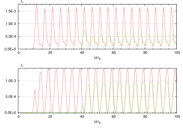
Figure 1: Luminosity as a function of normalized time $ct/r_{0}$. The top panel shows $L/(r_{0}B_{s})^{2}c$ for $\sigma_{0}/\nu=5$, and the bottom panel for $\sigma_{0}/\nu=0.5$. The two sinusoidal curves correspond to the values integrated at $r/r_{0}=10$ and $r/r_{0}=40$.

We examine the dependence of $\sigma_{0}$ on the luminosity in Fig. 2. Time-averaged values integrated at the surface corresponding to $r=\lambda$, $4\lambda$ and $8\lambda$ are denoted by $L_{1}$, $L_{4}$ and $L_{8}$ ($L_{1}>L_{4}>L_{8}$). The luminosities irrespective to the position ($r>\lambda$) approach $L_{*}\equiv 9.8\times 10^{-4}(r_{0}B_{s})^{2}c$ in the limit of small $\sigma_{0}$, where $L_{*}$ is the value of dipole radiation in vacuum, estimated in Eq. (27). All the values $L_{k}$ $(k=1,4,8)$ slightly decrease with increasing $\sigma_{0}$, but tend to increase for $\sigma_{0}/\nu>2$. The luminosity minimum is located near $\sigma_{0}/\nu\sim 2$. The dependence of $\sigma_{0}$ can be explained by two effects. One is the Ohmic dissipation:the decay timescale increases with it. The other is flowing currents produced in our model:the magnitude generally increases with $\sigma_{0}$. In the vacuum limit, $\sigma\equiv 0$, there are no currents and no dissipation of the electromagnetic energy. In the small region, the energy is quickly dissipated, and the reduction of the flux is more evident at great distances. With increase of $\sigma_{0}$, the Ohmic dissipation becomes less effective, and the amount of flowing currents increases. They produce electro-magnetic field structure different from that of vacuum in large $\sigma_{0}$ region. The induced fields dominate, and the outgoing flux is independent of the inner boundary condition as long as it is estimated outside the induction region.

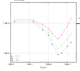
Figure 2: Time-averaged luminosity $L/(r_{0}B_{s})^{2}c$ as a function of parameter $2\sigma_{0}/\nu$. The arrow near the right-hand axis denotes the typical value $L_{*}$ by Eq.(27).

Figure 3 shows time evolution of electromagnetic fields. It is almost periodic, and the evolution during half of the oscillation period ($0.5\nu^{-1}=5r_{0}/c$) is shown. The top and bottom panels show the results for low conductivity ($\sigma_{0}/\nu=0.5$) and high conductivity ($\sigma_{0}/\nu=5$), respectively. The contours of the function $S(=B_{\phi}r\sin\theta)$ clearly represents a wave propagating at speed $c$. The oscillation behavior becomes apparent in the wave zone $r>\lambda=10r_{0}$. The angular dependence at which the amplitude is maximum on the equator forms a dipolar radiation pattern. Although octupole radiation may be involved, its effects are rather small. The magnetic flux function $G$ describing poloidal magnetic fields is also plotted. The pattern is dipolar in the inner region $r<10r_{0}$ but gradually deviates from this as the radius increases. This fact becomes much clearer at high conductivity. The contour of $G$ in Fig. 3 shows remarkable topological changes, i.e., reconnection due to resistivity: a small oval becomes detached from the outer part ($r\sim 15r_{0},\theta\sim\pi/2$) and shrinks beyond that region. In addition to the interesting behavior of poloidal fields, the magnitude of $B_{\phi}$ is considerably increased. Thus, poloidal and toroidal components of the magnetic fields are effectively coupled with each other through induced current at high conductivity. The induced current disappears at larger radii in our model ($\sigma\to 0$), and the magnetic field eventually becomes dipolar with some radiative component at infinity.

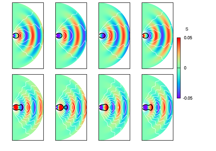
Figure 3: Time evolution of toroidal and poloidal magnetic fields in meridional plane ($0\leq\theta\leq\pi$ and $r\leq 25r_{0}=2.5\lambda$). Color contour represents $S(=B_{\phi}r\sin\theta)$ normalized by $B_{s}r_{0}$. Lines represent the level of the magnetic function $G/(B_{0}r_{0}^{2}$) for $0.03\times n(n=1,2,\cdots,7)$. The innermost contour line is written in black. Contours of larger $G$ within it, which are almost unchanged, are omitted. The top and bottom panels show the results for low conductivity ($\sigma_{0}/\nu=0.5$), and high conductivity ($\sigma_{0}/\nu=5$), respectively. From left to right, the panels correspond to $ct/r_{0}=$ 50.0, 51.7, 53.3 and 55.0.

4 Discussion

We studied time variation in a magnetosphere disturbed by torsional shear oscillation by using resistive electrodynamics. In this formalism, the current is described by Ohm’s law and the conductivity, and the electromagnetic fields are solved numerically. The results indicate that the induced current increases with the increase in conductivity, the fields are substantially modified, and the energy flux is thereby increased. Beyond a certain critical value of the conductivity $\sigma_{0}/\nu\sim{\mathcal{O}}(1)$, induced components dominate, and the inner boundary condition becomes less important. The behavior is however localized since the induced current disappears in the outer part. The exterior is assumed to approach vacuum in our model, in which the conductivity approaches zero. The extent of energy loss in the form of radiation is almost the same as that in vacuum. It is interesting to compare our results with those for a pulsar magnetosphere by Li et al. (2012), where the conductivity is assumed to be uniform everywhere. The results in Li et al. (2012) show that the luminosity increases with conductivity and approaches that of force-free calculation in the limit of high conductivity ($\sigma_{0}/\nu\gg 1$). Mathematically, the force-free limit is written as $\sigma\to\infty$ and $E_{0}\to 0$, but $\sigma E_{0}$ is finite in Eq. (17). In our numerical simulation, we found that $E_{0}$ does not necessarily approach zero everywhere ($E_{0}B_{0}=\vec{E}\cdot\vec{B}\neq 0$). The electromagnetic wave components $\vec{E}_{w}$ and $\vec{B}_{w}$ satisfy $\vec{E}_{w}\cdot\vec{B}_{w}=0$, however, there is another dipole component $\vec{B}_{d}$, for which $\vec{E}_{w}\cdot\vec{B}_{d}\neq 0$. It is not clear whether the problem arising in the limit of high conductivity depends on the spatial distribution model or on the numerical method.

The electric conductivity differs depending on the direction in the strongly magnetized regime, in which case the isotropic form of Ohm’s law (14) may be replaced by a tensor. As a brief discussion of directional differences, the conductivity is assumed to arise from collisions, and some terms in the generalized Ohm’s law are ignored. The conductivity parallel to the magnetic field is given by $\sigma_{\parallel}=e^{2}n_{e}/(m_{e}\nu_{c})$, and that in perpendicular direction is given by $\sigma_{\perp}=\sigma_{\parallel}/(1+(\omega_{B}/\nu_{c})^{2})$, where $\omega_{B}=eB/(m_{e}c)$ is the magnetic gyro-frequency and $\nu_{c}$ is the collision frequency (e.g., Somov (2006)). Using the Goldreich-Julian number density $n_{e}=B\nu/(ec)$, the ratio is reduced to $\sigma_{\perp}/\sigma_{\parallel}$ $=(1+(\sigma_{\parallel}/\nu)^{2})^{-1}$. The isotropic form may be no longer valid in the limit of $\sigma_{\parallel}/\nu\gg 1$, where $\sigma_{\parallel}\gg\sigma_{\perp}$. In our numerical simulation, the parameter is limited to $\sigma_{0}/\nu<10$. The anisotropic form of Ohm’s law would be adequate for larger values of to $\sigma_{0}/\nu$. Thus, conductivity is an important factor, but its magnitude and spatial distribution are poorly understood at present. A more elaborate treatment is necessary for constructing a more realistic model.

The outgoing energy flux is essential for estimating the damping mechanism of the oscillations. The luminosity $L$ calculated in this paper is of the same order as that in vacuum, although it depends on the conductivity. Appropriate scaling of the shear oscillation with $l=2$ leads to $L\sim 2\times 10^{37}$ $(\nu/30{\rm Hz})^{4}(\epsilon/10^{-2})^{2}(B/10^{14}{\rm G})^{2}$ ergs s^-1. The damping timescale for the energy $E\sim 10^{45}$ergs is $t_{d}=E/L$ $\sim$ a few years. This is a rather long period. It is difficult to significantly increase radiation loss, even if there exists a magnetosphere. The loss to infinity is not so efficient in the exterior vacuum region. The oscillation energy slowly escapes into the radiative zone, which is located beyond the region corresponding to a few wavelengths. In the presence of a magnetosphere, both ingoing and outgoing fluxes are likely to be produced due to interaction inside that zone, and current flows also change direction there. The inward energy flux and return current flows may be non-negligible in magnitude and may be dissipated as Joule heating in the region with higher resistance. Thus, the problem is extended to a globally coupled system between a neutron star/crust and a magnetosphere, which is more complex to model. The dynamics of coupled oscillations is an interesting topic for future research.

A model of a twisted magnetosphere would be more realistic since global electric current flows through the stellar surface(Thompson et al., 2002; Beloborodov & Thompson, 2007). The exterior of a star before flares is modeled by a purely dipole field, and in the present model current flows are allowed only during the oscillations. However, the effects of twisting may be significant. An interesting simulation by using a time-dependent force-free electrodynamics model was recently presented in Parfrey et al. (2012), where the evolution of the twisted magnetosphere was calculated. It was found that slow shearing at the surface leads to twisting and an abrupt reconnection. The evolutionary time scale ($\gg 1$ s) of that model is longer than that of ours ($<1$ s). Such a gradual twisting process would also be an interesting topic for future research.

References

- Abdikamalov et al. (2009) Abdikamalov E. B., Ahmedov B. J., Miller J. C., 2009, MNRAS, 395, 443
- Beloborodov & Thompson (2007) Beloborodov A. M., Thompson C., 2007, ApJ, 657, 967
- Cerdá-Durán et al. (2009) Cerdá-Durán P., Stergioulas N., Font J. A., 2009, MNRAS, 397, 1607
- Colaiuda & Kokkotas (2011) Colaiuda A., Kokkotas K. D., 2011, MNRAS, 414, 3014
- Duncan (1998) Duncan R. C., 1998, ApJ, 498, L45
- Gabler et al. (2012) Gabler M., Cerdá-Durán P., Stergioulas N., Font J. A., Müller E., 2012, MNRAS, 421, 2054
- Goldreich & Julian (1969) Goldreich P., Julian W. H., 1969, ApJ, 157, 869
- Gruzinov (2011) Gruzinov A., 2011, arXiv:1101.3100
- Israel et al. (2005) Israel G. L., Belloni T., Stella L., Rephaeli Y., Gruber D. E., Casella P., Dall’Osso S., Rea N., Persic M., Rothschild R. E., 2005, ApJ, 628, L53
- Jackson (1975) Jackson J. D., 1975, Classical electrodynamics
- Kalapotharakos et al. (2012) Kalapotharakos C., Kazanas D., Harding A., Contopoulos I., 2012, ApJ, 749, 2
- Lee (2008) Lee U., 2008, MNRAS, 385, 2069
- Levin (2007) Levin Y., 2007, MNRAS, 377, 159
- Li et al. (2012) Li J., Spitkovsky A., Tchekhovskoy A., 2012, ApJ, 746, 60
- McDermott et al. (1984) McDermott P. N., Savedoff M. P., van Horn H. M., Zweibel E. G., Hansen C. J., 1984, ApJ, 281, 746
- Mereghetti (2008) Mereghetti S., 2008, A&AR, 15, 225
- Morozova et al. (2010) Morozova V. S., Ahmedov B. J., Zanotti O., 2010, MNRAS, 408, 490
- Parfrey et al. (2012) Parfrey K., Beloborodov A. M., Hui L., 2012, ApJ, 754, L12
- Piro (2005) Piro A. L., 2005, ApJ, 634, L153
- Somov (2006) Somov B. V., ed. 2006, Plasma astrophysics, part I : fundamentals and practice Vol. 340 of Astrophysics and Space Science Library
- Sotani et al. (2008) Sotani H., Kokkotas K. D., Stergioulas N., 2008, MNRAS, 385, L5
- Strohmayer & Watts (2006) Strohmayer T. E., Watts A. L., 2006, ApJ, 653, 593
- Thompson et al. (2002) Thompson C., Lyutikov M., Kulkarni S. R., 2002, ApJ, 574, 332
- Timokhin et al. (2000) Timokhin A. N., Bisnovatyi-Kogan G. S., Spruit H. C., 2000, MNRAS, 316, 734
- Unno et al. (1989) Unno W., Osaki Y., Ando H., Saio H., Shibahashi H., 1989, Nonradial oscillations of stars
- van Hoven & Levin (2012) van Hoven M., Levin Y., 2012, MNRAS, 420, 3035