Autocorrelation function of velocity increments time series in fully developed turbulence

Abstract

In fully developed turbulence, the velocity field possesses long-range correlations, denoted by a scaling power spectrum or structure functions. Here we consider the autocorrelation function of velocity increment ${\Delta u_{\ell}(t)}$ at separation time $\ell$. Anselmet et al. [Anselmet et al. J. Fluid Mech. 140, 63 (1984)] have found that the autocorrelation function of velocity increment has a minimum value, whose location is approximately equal to $\ell$. Taking statistical stationary assumption, we link the velocity increment and the autocorrelation function with the power spectrum of the original variable. We then propose an analytical model of the autocorrelation function. With this model, we prove that the location of the minimum autocorrelation function is exactly equal to the separation time $\ell$ when the scaling of the power spectrum of the original variable belongs to the range $0<\beta<2$. This model also suggests a power law expression for the minimum autocorrelation. Considering the cumulative function of the autocorrelation function, it is shown that the main contribution to the autocorrelation function comes from the large scale part. Finally we argue that the autocorrelation function is a better indicator of the inertial range than the second order structure function.

1 Introduction

Turbulence is characterized by power law of the velocity spectrum [1] and structure functions in the inertial range [2, 3]. This is associated to long-range power-law correlations for the dissipation or absolute value of the velocity increment. Here we consider the autocorrelation of velocity increments (without absolute value), inspired by a remark found in Anselmet et al. (1984) [4]. In this reference, it is found that the location of the minimum value of the autocorrelation function $\Gamma(\tau)$ of velocity increment $\Delta u_{\ell}(t)$, defined as

$$\Delta u_{\ell}(t)=u(t+\ell)-u(t)$$ (1)

of fully developed turbulence with time separation $\ell$ is approximately equal to $\ell$. The autocorrelation function of this time series is defined as

$$\Gamma(\tau)={\langle(V_{\ell}(t)-\mu)(V_{\ell}(t-\tau)-\mu)\rangle}$$ (2)

where $V_{\ell}(t)=\Delta u_{\ell}(t)$, $\mu$ is the mean value of $V$, and $\tau>0$ is the time lag.

This paper mainly presents analytical results. In first section we present the database considered here as an illustration of the property which is studied. The next section presents theoretical studies. The last section provides a discussion.

Figure 1: Compensated spectrum $E(f)f^{\beta}$ of streamwise (longitudinal) ($\beta\simeq 1.63$) and spanwise (transverse)($\beta\simeq 1.62$) velocity, where $\beta$ is the corresponding power law estimated from the power spectrum. The plateau is observed on the range $20<f<2000$ Hz and $40<f<4000$ Hz for streamwise (longitudinal) and spanwise (transverse) velocity, respectively.

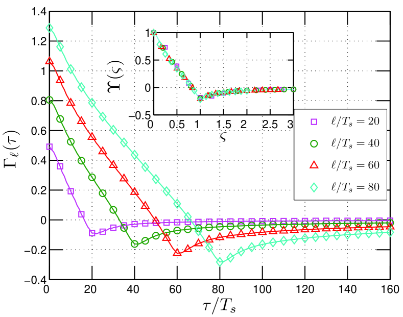
Figure 2: Autocorrelation function $\Gamma_{\ell}(\tau)$ of the velocity increment $\Delta u_{\ell}(t)$ estimated from an experimental homogeneous and nearly isotropy turbulence time series with various increments $\ell$. The location of the minimum value is very close to the separation time $\ell$. The inset shows the rescaled autocorrelation function $\Upsilon(\varsigma)$.

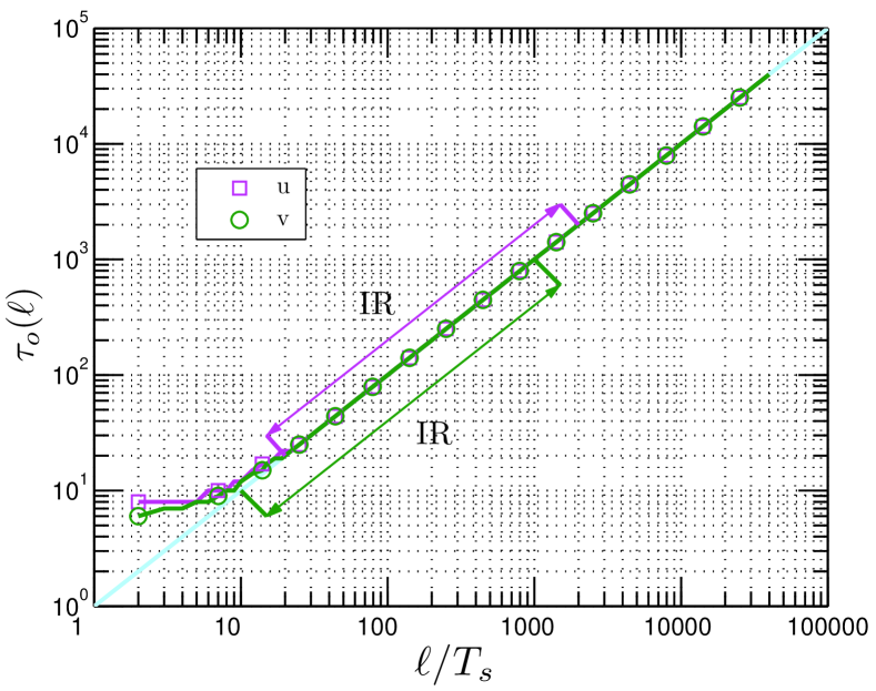
Figure 3: Location $\tau_{o}(\ell)$ of the minimum value of the autocorrelation function estimated from experimental data, where the inertial range is marked as IR. The solid line indicates $\tau_{o}(\ell)=\ell$.

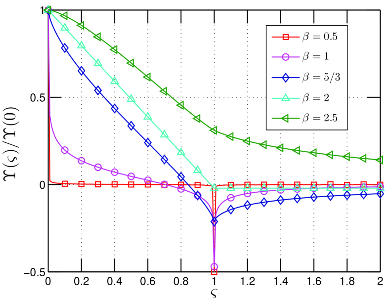
Figure 4: Numerical solution of the rescaled autocorrelation function $\Upsilon(\varsigma)$ with various $\beta$ from 0.5 to 2.5 estimated from eq. (10).

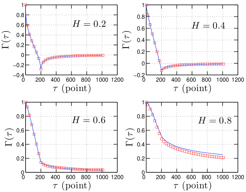
Figure 5: Comparison of the autocorrelation function, which is predicted by eq. (20) (solid line) and estimated from fBm simulation ($\square$) with $\ell=200$ points.

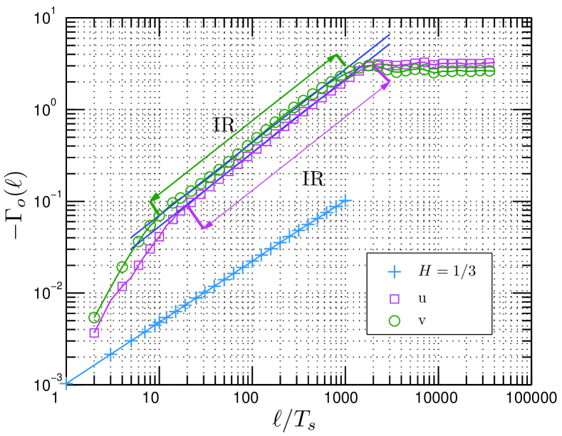
Figure 6: Representation of the minima value $\Gamma_{o}(\ell)$ of the autocorrelation function estimated from synthesized fBm time series with $H=1/3$ ($+$), and the experimental data for streamwise (longitudinal) ($\square$) and spanwise (transverse) ($\ocircle$) turbulent velocity components, where the corresponding inertial range is denoted as IR. Power law behaviour is observed with scaling exponent $\beta-1=2/3$ and $\beta-1=0.78\pm 0.04$ for fBm and turbulent velocity, respectively.

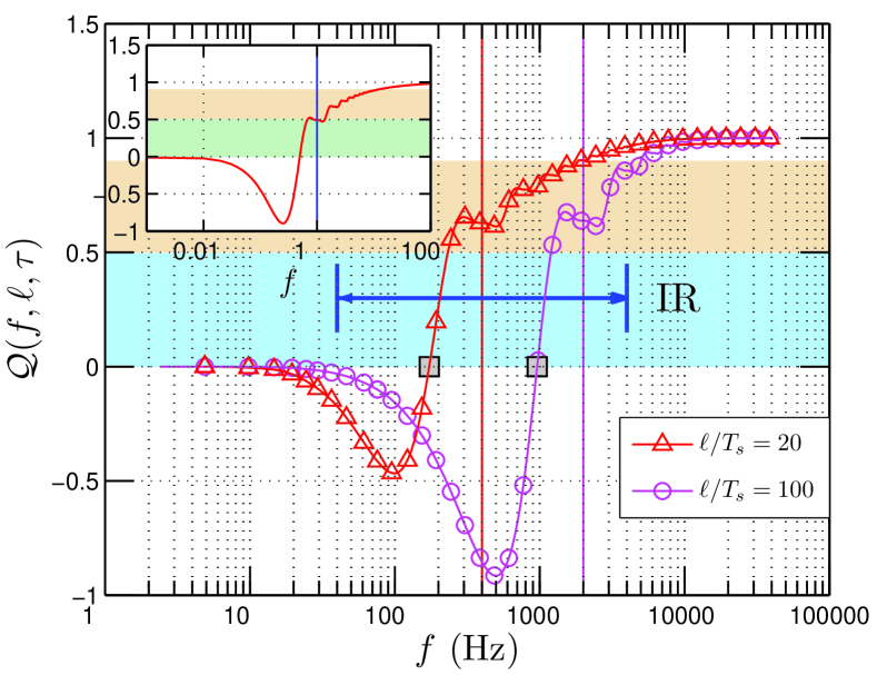
Figure 7: Cumulative function $\mathcal{Q}(f,\ell,\tau)$ estimated from turbulent experimental data for spanwise (transverse) velocity with $\tau=\ell$ in the inertial range, where the numerical solution is shown as inset with $\ell=1$. The inertial range is denoted as IR. Vertical solid lines demonstrate the corresponding scale in spectral space.

Figure 8: Cumulative function $\mathcal{Q}_{1}(f)$ estimated from turbulent experimental data for both streamwise (longitudinal) and spanwise (transverse) velocity with various $\ell$. The numerical solution is $\mathcal{Q}_{1}\simeq 0.5$.

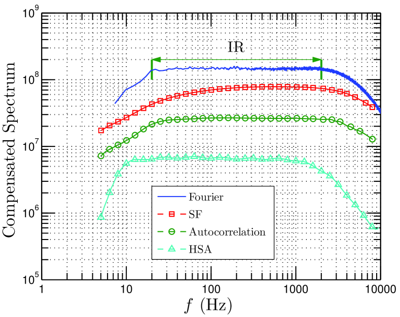
Figure 9: Comparison of the inertial range for the streamwise (longitudinal) velocity. They are estimated directly by the Fourier power spectrum, the second order structure function,the Hilbert spectral analysis and the autocorrelation function.

2 Experimental analysis of the autocorrelation function of velocity increments

We consider here a turbulence velocity time series obtained from an experimental homogeneous and nearly isotropic turbulent flow at downstream $x/M=20$, where $M$ is the mesh size. The flow is characterized by the Taylor microscale based Reynolds number $Re_{\lambda}=720$[5]. The sampling frequency is $f_{s}=40\,$kHz and a low-pass filter at a frequency $20\,$kHz is applied on the experimental data. The sampling time is $30\,$s, and the number of data points per channel for each measurement is $1.2\times 10^{6}$. We have 120 realizations with four channels. The total number of data points at this location is $5.76\times 10^{8}$. The mean velocity is $12\,\mathrm{ms^{-1}}$. The rms velocity is 1.85 and $1.64\,\mathrm{ms^{-1}}$ for streamwise (longitudinal) and spanwise (transverse) velocity component. The Kolmogorov scale $\eta$ and the Taylor microscale $\lambda$ are 0.11 mm and 5.84 mm respectively. Let us note here $T_{s}=1/f_{s}$ time resolution of these measurements. This data demonstrates an inertial range over two decades [5], see a compensated spectrum $E(f)f^{\beta}$ in fig. 1, where $\beta\simeq 1.63$ and $\beta\simeq 1.62$ for streamwise (longitudinal) and spanwise (transverse) velocity respectively. We show the autocorrelation function $\Gamma_{\ell}(\tau)$ directly estimated from these data in fig. 2. Graphically, the location $\tau_{o}$ of the minimum value of each curve is very close to $\ell$, which confirms Anselmet’s observation [4]. Let us define

$$\Gamma_{o}(\ell)=\min_{\tau}\{\Gamma_{\ell}(\tau)\}$$ (3)

and $\tau_{o}$ the location of the minimum value

$$\Gamma_{o}(\ell)=\Gamma_{\ell}(\tau_{o}(\ell))$$ (4)

We show the estimated $\tau_{o}(\ell)$ on the range $2<\ell/T_{s}<40000$ in fig. 3, where the inertial range is indicated by IR. It shows that when $\ell$ is greater than $20T_{s}$, $\tau_{o}$ is very close to $\ell$ even when $\ell$ is in the forcing range, in agreement with the remark of Anselmet et al. [4]. In the following, we show this analytically.

3 Autocorrelation function

Considering the statistical stationary assumption[3], we represent $u(t)$ in Fourier space, which is written as

$$\hat{U}(f)=\mathcal{F}(u(t))=\int_{-\infty}^{+\infty}u(t)e^{-2\pi ift}\upd t$$ (5)

where $\mathcal{F}$ means Fourier transform and $f$ is the frequency. Thus, the Fourier transform of the velocity increment $\Delta u_{\ell}(t)$ is written as

$${S}_{\ell}(f)=\mathcal{F}({\Delta u_{\ell}(t)})=\hat{U}(f)(e^{2\pi if\ell}-1)$$ (6)

where $\Delta u_{\ell}(t)=u(t+\ell)-u(t)$. Hence, the 1D power spectral density function of velocity increments $E_{\Delta}(f)$ is expressed as

$$E_{\Delta}(f)=|S_{\ell}(f)|^{2}=E_{v}(f)(1-\cos(2\pi f\ell))$$ (7)

where $E_{v}(f)=2|\hat{U}(f)|^{2}$ is the velocity power spectrum [3]. It is clear that the velocity increment operator acts a kind of filter, where the frequencies $f_{\Delta}=n/\ell$, $n=0,1,2\cdots$, are filtered.

Let us consider now the autocorrelation function of the increment. The Wiener-Khinchin theorem relates the autocorrelation function to the power spectral density via the Fourier transform[6, 3]

$$\Gamma_{\ell}(\tau)=\int_{0}^{+\infty}E_{\Delta}(f)\cos(2\pi f\tau)\upd f$$ (8)

The theorem can be applied to wide-sense-stationary random processes, signals whose Fourier transforms may not exist, using the definition of autocorrelation function in terms of expected value rather than an infinite integral[6]. Substituting eq. (7) into the above equation, and assuming a power law for the spectrum (a hypothesis of similarity)

$$E_{v}(f)=cf^{-\beta},\quad c>0$$ (9)

we obtain

$$\Gamma_{\ell}(\tau)=c\int_{0}^{+\infty}f^{-\beta}(1-\cos(2\pi f\ell))\cos(2\pi f\tau)\upd f$$ (10)

The convergence condition requires $0<\beta<3$. It implies a rescaled relation, using scaling transformation inside the integral. This can be estimated by taking $\ell^{\prime}=\lambda\ell$, $f^{\prime}=f\lambda$, $\tau^{\prime}=\tau/\lambda$ for $\lambda>0$, providing the identity

$$\Gamma_{\lambda\ell}(\tau)=\Gamma_{\ell}(\tau/\lambda)\lambda^{\beta-1}$$ (11)

If we take $\ell=1$ and replace $\lambda$ by $\ell$, we then have

$$\Gamma_{\ell}(\tau)=\Gamma_{1}(\tau/\ell)\ell^{\beta-1}$$ (12)

Thus, we have a universal autocorrelation function

$${\Gamma_{\ell}(\ell\varsigma)}{\ell^{1-\beta}}=\Upsilon(\varsigma)=\Gamma_{1}(\varsigma)$$ (13)

This rescaled universal autocorrelation function is shown as inset in fig. 2. A derivative of eq. (11) gives $\Gamma^{\prime}_{\lambda\ell}(\tau)=\Gamma^{\prime}_{\ell}(\tau/\lambda)\lambda^{\beta-2}$. The minimum value of the left-hand side is $\tau=\tau_{o}(\lambda\ell)$, verifying $\Gamma^{\prime}_{\lambda\ell}(\tau_{o}(\lambda\ell))=0$ and for this value we have also $\Gamma^{\prime}_{\ell}(\tau_{o}(\lambda\ell)/\lambda)=0$. This shows that $\tau_{o}(\ell)=\tau_{o}(\lambda\ell)/\lambda$. Taking again $\ell=1$ and $\lambda=\ell$, we have

$$\tau_{o}(\ell)=\ell\tau_{o}(1)$$ (14)

Showing that $\tau_{o}(\ell)$ is proportional to $\ell$ in the scaling range (when $\ell$ belongs to the inertial range). With the definition of $\Gamma_{o}(\ell)=\Gamma_{\ell}(\tau_{o}(\ell))$ we have, also using eq. (11), for $\tau=\tau_{o}(\lambda\ell)$:

$$\begin{array}[]{ll}\Gamma_{\lambda\ell}(\tau_{o}(\lambda\ell))&=\Gamma_{\ell}(\tau_{o}(\lambda\ell)/\lambda)\lambda^{\beta-1}\\ &=\Gamma_{\ell}(\tau_{o}(\ell))\lambda^{\beta-1}\end{array}$$ (15)

Hence $\Gamma_{o}(\lambda\ell)=\lambda^{\beta-1}\Gamma_{o}(\ell)$ or

$$\Gamma_{o}(\ell)=\Gamma_{o}(1)\ell^{\beta-1}$$ (16)

We now consider the location $\tau_{o}(1)$ of the autocorrelation function for $\ell=1$. We take the first derivative of eq. (10), written for $\ell=1$

$$\mathcal{P}(\tau)=\frac{\upd\Gamma_{1}(\tau)}{\upd\tau}=-\int_{0}^{+\infty}f^{1-\beta}(1-\cos(2\pi f))\sin(2\pi f\tau)\upd f$$ (17)

where we left out the constant in the integral. The same rescaling calculation leads to the following expression

$$\begin{array}[]{l}\mathcal{P}(\tau)=\left[(1+1/\tau)^{\beta-2}+(1-1/\tau)^{\beta-2}-2\right]M/2,\tau\neq 1\\ \mathcal{P}(\tau)=\left(2^{\beta-3}-1\right)M,\quad\quad\tau=1\end{array}$$ (18)

where $M=\int_{0}^{+\infty}x^{1-\beta}(1-\cos(2\pi x))\sin(2\pi x\tau)\upd x$ and $M>0$ [7]. The convergence condition requires $1<\beta<4$. When $\beta<2$, one can find that both left and right limits of $\mathcal{P}(1)$ are infinite, but the definition of $\mathcal{P}(1)$ in eq. (17) is finite. Thus $\tau=1$ is a second type discontinuity point of eq. (17) [8]. It is easy to show that

$$\left\{\begin{array}[]{rl}&\mathcal{P}(\tau)<0,\tau\leq 1\\ &\mathcal{P}(\tau)>0,\tau>1\end{array}\right.$$ (19)

It means that $\mathcal{P}(\tau)$ changes its sign from negative to positive when $\tau$ is increasing from $\tau<1$ to $\tau>1$. In other words the autocorrelation function will take its minimum value at the location where $\tau$ is exactly equal to $1$. We thus see that $\tau_{o}(1)=1$ and hence $\tau_{o}(\ell)=\ell$ (eq. (14)).

4 Numerical validation

There is no analytical solution for eq. (10). It is then solved here by a proper numerical algorithm. We perform a fourth order accurate Simpson rule numerical integration of eq. (10) on range $10^{-4}<f<10^{4}$ with $\ell=1$ for various $\beta$ with step $\Delta f=10^{-6}$. We show the rescaled numerical solutions $\Upsilon(\varsigma)$ for various $\beta$ values in fig. 4. Graphically, as what we have proved above, the location $\tau_{o}(1)$ of the minimum autocorrelation function is exactly equal to $1$ when $0<\beta<2$.

For the fBm, the autocorrelation function of the increments is known to be the following [9]

$$\Gamma_{\ell}(\tau)=\frac{1}{2}\left\{(\tau+\ell)^{2H}+|\tau-\ell|^{2H}-\tau^{2H}\right\}$$ (20)

where $\tau\geq 0$. We compare the autocorrelation (coefficient) function estimated from fBm simulation ($\square$, see bellow) with eq. (20) (solid line) in fig. 5, where $\ell=200$ points. Graphically, eq. (20) provides a very good prediction with numerical simulation. Based on this model, it is not difficult to find that $\Gamma_{o}(\ell)\sim\ell^{2H}$ when $0<H<1$, corresponding to $1<\beta<3$, and $\tau_{o}(\ell)=\ell$ when $0<H<0.5$, corresponding to $1<\beta<2$. One can find that the validation range of scaling exponent $\beta$ is only a subset of Wiener-Khinchin theorem.

We then check the power law for the minimum value of the autocorrelation function given in eq. (12). We simulate 100 segments of fractional Brownian motion with length $10^{6}$ data points each, by performing a Wavelet based algorithm [10]. We take db2 wavelet with $H=1/3$ (corresponding to the Hurst number of turbulent velocity). We plot the estimated minima value $\Gamma_{o}(\ell)$ ($+$) of the autocorrelation function in fig. 6. A power law behaviour is observed with the scaling exponent $\beta-1=2/3$ as expected. It confirms eq. (12) for fBm. We also plot $\Gamma_{o}(\ell)$ estimated from turbulent experimental data for both streamwise (longitudinal) ($\square$) and spanwise (transverse) ($\ocircle$) velocity components in fig. 6, where the inertial range is marked by IR. Power law is observed on the corresponding inertial range with scaling exponent $\beta-1=0.78\pm 0.04$. Due to the intermittency, this scaling exponent is larger than 2/3. The exact relation between this scaling exponent with intermittent parameter should be investigated further in future. The power law range is almost the same as the inertial range estimated by Fourier power spectrum. It indicates that autocorrelation function can be used to determine the inertial range. Indeed, as we show later, it seems to be a better inertial range indicator than structure function.

5 Discussion

We define a cumulative function

$$\mathcal{Q}(f,\ell,\tau)=\frac{\int_{0}^{f}K(f^{\prime},\ell,\tau)\upd f^{\prime}}{\int_{0}^{+\infty}K(f^{\prime},\ell,\tau)\upd f^{\prime}}$$ (21)

where

$$K(f,\ell,\tau)=E_{\Delta}(f)\cos(2\pi f\tau)$$ (22)

is the integration kernel of eq. (8). It measures the contribution of the frequency from 0 to $f$ at given scale $\ell$ and time delay $\tau$. We are particularly concerned by the case $\tau=\ell$. To avoid the effects of the measurement noise, see fig. 1, we only consider here the spanwise (transverse) velocity. We show the estimated $\mathcal{Q}$ in fig. 7 for two scales $\ell/T_{s}=20$ ($\ocircle$) and $\ell/T_{s}=100$ ($\triangle$) in the inertial range, where the vertical solid line illustrates the location of the corresponding time scale in spectral space. In these experimental curves, the kernel $K$ given in eq. (21) is computed using the experimental spectrum $E_{v}(f)$. The corresponding inertial range is denoted by IR. We also show the numerical solution of eq. (21) with $\ell=1$ as inset , which is estimated by taking a pure power law $E_{v}(f)\sim f^{-\beta}$ in eq. (21). We notice that both curves cross the line $\mathcal{Q}=0$. We denote $f_{o}$ such as $\mathcal{Q}(f_{o})=0$. It has an advantage that the contribution from large scale $\ell>1/f_{o}$ is canceled by itself. Graphically, in the inertial range, the distance between $f_{o}$ and the corresponding scale $\ell$ is less than 0.3 decade. The numerical solution indicates that this distance is about 0.3 decade. We then separate the contribution into a large scale part and a small scale part. We denote the contribution from the large scale part as $\mathcal{Q}_{1}(f)=\mathcal{Q}(1/\ell,\ell,\ell)$. The experimental result is shown in fig. 8 for both streamwise (longitudinal) and spanwise (transverse) velocity components. The mean contribution from large scale is found graphically to be 0.64. It is significantly larger than 0.5, the value indicated by the numerical solution. It means that the autocorrelation function is influenced more by the large scale than by the small scale.

We now consider the inertial range provided by different methods. We replot the corresponding compensated spectra estimated directly by Fourier power spectrum (solid line), the second order structure function ($\square$), the autocorrelation function ($\ocircle$) and the Hilbert spectral analysis ($\triangle$) [11] in fig. 9 for streamwise (longitudinal)velocity. For comparison convenience, both the structure function and the autocorrelation function are converted from physical space into spectral space by taking $f=1/\ell$. For display convenience, these curves are vertically shifted. Graphically, except the structure function, the other lines demonstrate a clear plateau. As we have pointed above, the autocorrelation function is a better indicator of the inertial range than structure function. We also notice that the inertial range provided by the Hilbert methodology is slightly different from the Fourier spectrum. This may come from the fact that the former methodology has a very local ability both in physical and spectral domain [11, 12], thus the large scale effect should be constrained. However, the Fourier analysis requires the stationary of the data, which is obviously not satisfied by the turbulence data. The result we present here can also be linked with intermittency property of turbulence: we will present this in future work.

6 Conclusion

In this work, we considered the autocorrelation function of the velocity increment $\Delta u_{\ell}(t)$ time series, where $\ell$ is a time scale. Taking statistical stationary assumption, we propose an analytical model of the autocorrelation function. With this model, we proved analytically that the location of the minimum autocorrelation function is exactly equal to the separation time scale $\ell$ when the scaling of the power spectrum of the original variable belongs to the range $0<\beta<2$. In fact, this property was found experimentally to be valid outside the scaling range, but our demonstration here concerns only the scaling range. This model also suggests a power law expression for the minimum autocorrelation $\Gamma_{o}(\ell)$. Considering the cumulative integration of the autocorrelation function, it was shown that the autocorrelation function is influenced more by the large scale part. Finally we argue that the autocorrelation function is a better indicator of the inertial range than second order structure function. These results have been illustrated using fully developed turbulence data; however, they are of more general validity since we only assumed that the considered time series is stationary and possesses scaling statistics.

- [1] \NameKolmogorov A. N. \REVIEWDokl. Akad. Nauk SSSR 301941299.
- [2] \NameMonin A. S. Yaglom A. M. \BookStatistical fluid mechanics (MIT Press Cambridge, Mass) 1971.
- [3] \NameFrisch U. \BookTurbulence: the legacy of AN Kolmogorov (Cambridge University Press) 1995.
- [4] \NameAnselmet F., Gagne Y., Hopfinger E. J. Antonia R. A. \REVIEWJ. Fluid Mech. 140198463.
- [5] \NameKang H., Chester S. Meneveau C. \REVIEWJ. Fluid Mech. 4802003129.
- [6] \NamePercival D. Walden A. \BookSpectral Analysis for Physical Applications: Multitaper and Conventional Univariate Techniques (Cambridge University Press) 1993.
- [7] \NameSamorodnitsky G. Taqqu M. \BookStable Non-Gaussian Random Processes: stochastic models with infinite variance (Chapman & Hall) 1994.
- [8] \NameMalik S. Arora S. \BookMathematical Analysis (John Wiley & Sons Inc) 1992.
- [9] \NameBiagini F., Hu Y., Oksendal B. Zhang T. \BookStochastic calculus for fractional Brownian motion and applications (Springer Verlag) 2008.
- [10] \NameAbry P. Sellan F. \REVIEWAppl. Comput. Harmon. Anal. 31996377.
- [11] \NameHuang Y., Schmitt F. G., Lu Z. Liu Y. \REVIEWEurophys. Lett. 84200840010.
- [12] \NameHuang Y., Schmitt F. G., Lu Z. Liu Y. \REVIEWTraitement du Signal (in press) 2009.