An amplitude-frequency study of turbulent scaling intermittency using Empirical Mode Decomposition and Hilbert Spectral Analysis

Abstract

Hilbert-Huang transform is a method that has been introduced recently to decompose nonlinear, nonstationary time series into a sum of different modes, each one having a characteristic frequency. Here we show the first successful application of this approach to homogeneous turbulence time series. We associate each mode to dissipation, inertial range and integral scales. We then generalize this approach in order to characterize the scaling intermittency of turbulence in the inertial range, in an amplitude-frequency space. The new method is first validated using fractional Brownian motion simulations. We then obtain a 2D amplitude-frequency representation of the pdf of turbulent fluctuations with a scaling trend, and we show how multifractal exponents can be retrieved using this approach. We also find that the log-Poisson distribution fits the velocity amplitude pdf better than the lognormal distribution.

1 Introduction

In nature and the real world, most data are nonlinear, nonstationary and noisy, and general data-driven methods to analyze such data, without a priori assumptions basis, are demanded. About ten years ago, such a method has been proposed to analyze nonlinear and nonstationary time series: Hilbert-Huang transform (hereafter HHT) [1, 2]. The first step of this method is the Empirical Mode Decomposition (EMD), which is used to decompose a time series into a sum of different time series (modes), each one having a characteristic frequency [3, 4]. The modes are called Intrinsic Mode Functions (IMFs) and satisfy the following two conditions: (i) the difference between the number of local extrema and the number of zero-crossings must be zero or one; (ii) the running mean value of the envelope defined by the local maxima and the envelope defined by the local minima is zero. Each IMF has a characteristic scale which is the mean distance between two successive maxima (or minima). The procedure to decompose a signal into IMFs is the following:

• The local extrema of the signal $X(t)$ are identified;

• The local maxima are connected together forming an upper envelope $e_{\max}(t)$, which is obtained by a cubic spline interpolation. The same is done for local minima, providing a lower envelope $e_{\min}(t)$;

• The mean is defined as $m_{1}(t)=(e_{\max}(t)+e_{\min}(t))/2$;

• The mean is subtracted from the signal, providing the local detail $h_{1}(t)=X(t)-m_{1}(t)$;

• The component $h_{1}(t)$ is then examined to check if it satisfies the conditions to be an IMF. If yes, it is considered as the first IMF and denoted $C_{1}(t)=h_{1}(t)$. It is subtracted from the original signal and the first residual, $r_{1}(t)=X(t)-C_{1}(t)$ is taken as the new series in step 1. On the other hand, if $h_{1}(t)$ is not an IMF, a procedure called “sifting process” is applied as many times as needed to obtain an IMF. The sifting process is the following: $h_{1}(t)$ is considered as the new data; the local extrema are estimated, lower and upper envelopes are formed and their mean is denoted $m_{11}(t)$. This mean is subtracted from $h_{1}(t)$, providing $h_{11}(t)=h_{1}(t)-m_{11}(t)$. Then it is checked again if $h_{11}(t)$ is an IMF. If not, the sifting process is repeated, until the component $h_{1k}(t)$ satisfies the IMF conditions. Then the first IMF is $C_{1}(t)=h_{1k}(t)$ and the residual $r_{1}(t)=X(t)-C_{1}(t)$ is taken as the new series in step 1.

The above sifting process should be stopped by a criterion which is not discussed here: more details about the EMD algorithm can be found in refs. [1, 2, 4, 5, 6].

After decomposition, the original signal $X(t)$ is written as a sum of IMF modes $C_{i}(t)$ and a residual $r_{n}(t)$

$$X(t)=\sum_{i=1}^{N}{C_{i}(t)}+r_{n}(t)$$ (1)

EMD is associated with Hilbert Spectral Analysis (HSA) [7, 8, 1], which is applied to each mode as a time frequency analysis, in order to locally extract a frequency and an amplitude. More precisely, each mode function $C(t)$ is associated with its Hilbert transform $\tilde{C}$

$$\tilde{C}(t)=\frac{1}{\pi}\int_{-\infty}^{+\infty}\frac{C(\tau)}{t-\tau}\,\upd\tau$$ (2)

and the combination of $C(t)$ and $\tilde{C}(t)$ gives the analytical signal $z=C+j\tilde{C}=\mathcal{A}(t)e^{j\theta(t)}$, where $\mathcal{A}(t)$ is an amplitude time series and $\theta(t)$ is the phase of the mode oscillation [7]. Within such approach and neglecting the residual, the original time series is rewritten as

$$X(t)=Re\sum_{i=1}^{N}{\mathcal{A}_{i}(t)}e^{j\theta_{i}(t)}$$ (3)

where $\mathcal{A}_{i}$ and $\theta_{i}$ are the amplitude and phase time series of mode $i$ and $Re$ means real part [1, 2]. For each mode, the Hilbert spectrum is defined as the square amplitude $H(\omega,t)=\mathcal{A}^{2}(\omega,t)$, where $\omega=d\theta/dt$ is the instantaneous frequency extracted using the phase information $\theta(t)=\tan^{-1}\tilde{C}(t)/C(t)$. $H(\omega,t)$ gives a local representation of energy in the time-frequency domain. The Hilbert marginal spectrum of the original time series is then written as $h(\omega)=\int H(\omega,t)\,\upd t$ and corresponds to an energy density at frequency $\omega$ [8, 1, 2].

Since its introduction, this method has attracted a large interest [9]. It was shown to be an efficient method to separate a signal into a trend and small scale fluctuations on a dyadic bank [3, 4, 5]; it has also been applied to many fields including physiology [10], geophysics [11], climate studies [12], mechanical engineering [13] and acoustics [14], to quote a few. These studies showed the applicability of the so-called EMD-HSA approach on many different time series. In this letter, we apply the EMD and HSA approaches to fully developed turbulence time series. We first show that the EMD method applies very nicely to turbulent velocity time series, with an almost dyadic filter bank in the inertial range. We then show how the HSA can be generalized to take into account intermittency. We apply this to the turbulence time series, providing a first characterization of the intermittency of turbulence in an amplitude-frequency representation.

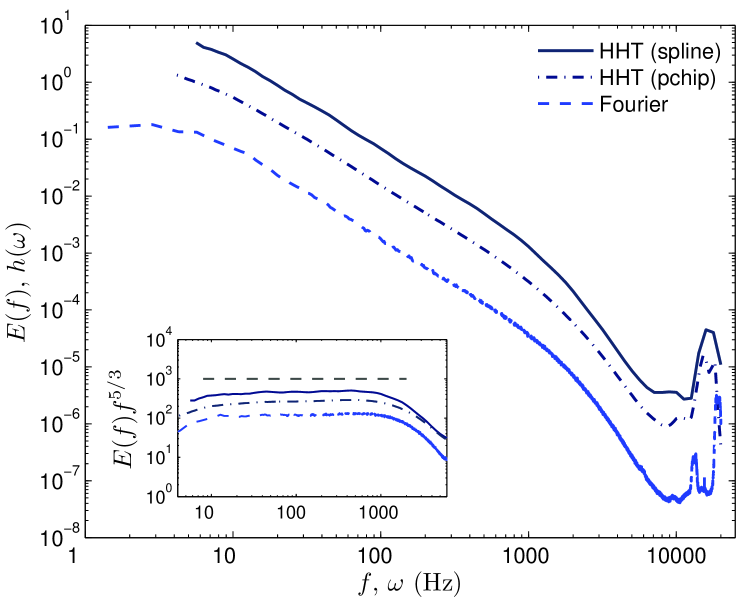
Figure 1: Comparison of the Hilbert marginal energy spectrum (solid line) and Fourier spectrum (dashed line, vertically shifted). The slope of the reference line is $-5/3$. Both the second order Hilbert and Fourier spectra indicate the same inertial subrange, $10<f\,(\textrm{or }\omega)<1000\,\textrm{Hz}$. The insert shows the compensated spectra. The HHT spectra estimated using two different algorithms are shown for comparison, indicating a stability of the spectrum with respect to the algorithm used.

2 Application of EMD to turbulence time series

We consider here a database obtained from measurements of nearly isotropic turbulence downstream an active-grid characterized by the Reynolds number $Re_{\lambda}=720$. The sampling frequency is $f_{\mathrm{s}}=40\un{kHz}$ [15]. The sampling time is $30\un{s}$ , and the total number of data points per channel for each measurement is $1.2\times 10^{6}$. We consider data in the streamwise direction at position $x/M=48$, where $M$ is the mesh size and $x$ is the distance in the streamwise direction. The mean velocity at this location is $10.8\un{ms^{-1}}$ and the turbulence intensity is about $10\%$. For details about the experiment and the data see ref. [15].

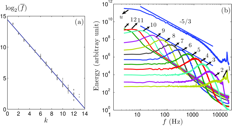
Figure 2: (a) Mean frequency versus mode number for the turbulent velocity time series. There is an exponential decrease with a slope very close to 1. This indicates that EMD acts as a filter bank which is almost dyadic. (b) Fourier spectrum of each mode (from 1 to 12) showing that they are narrow-banded. The slope of the reference line is $-5/3$ corresponding to the inertial-range Kolmogorov spectrum.

Figure 1 shows the second order Hilbert and Fourier spectra of the longitudinal velocity. A Kolmogorov $-5/3$ spectrum is observed in range $10<f\,(\textrm{or }\omega)<1000\un{Hz}$ for both spectra, indicating an inertial subrange over 2 decades. Two different HHT spectra estimated using two different algorithms are shown in this figure: the very similar shape of the spectra indicates a stability of the spectrum with respect to the algorithm used. The scaling which is obtained shows that Hilbert spectral analysis can be used to recover Kolmogorov scaling in the inertial subrange. The original velocity time series is divided into 73 non-overlapping segments of $2^{14}$ points each. After decomposition, the original velocity series is decomposed into several IMFs from 11 to 13 modes with one residual. The time scale is increasing with the mode; each mode has a different mean frequency, which is estimated by considering the (energy weighted) mean frequency in the Fourier power spectrum. The relation between mode number $k$ and mean frequency [1] is displayed in fig. 2 (a). The straight line in log-linear plot which is obtained suggests the following relation $\overline{f}(k)=f_{0}\rho^{-k}$, where $\overline{f}$ is the mean frequency, $f_{0}\simeq 22000$ is a constant and $\rho=1.9\pm 0.1$ is very close to 2, the slight discrepancy from 2 may be an effect of intermittency. This result may also slightly depend on the number of iterations of the sifting process: in the present algorithm, the latter is variable but some proposed algorithms contain a fixed maximum number of iterations.

This indicates that EMD acts as a dyadic filter bank in the frequency domain; an analogous property was obtained previously using stochastic simulations of Gaussian noise and fractional Gaussian noise (fGn) [4, 5, 3], and it is interesting to note here that the same result holds for fully developed turbulence time series, possessing long-range correlations and intermittency [16].

We then interpret each mode according to its characteristic time scale. When compared with the original Fourier spectrum of the turbulent time series (see fig. 2 (b)), these modes can be termed as follows: the first mode, which has the smallest time scale, corresponds to the measurement noise; modes 2 and 3 are associated with the dissipation range of turbulence. Mode 4 corresponds to the Kolmogorov scale, which is the scale below which dissipation becomes important; it is a transition scale between inertial range and dissipation range. Modes 5 to 10 all belong to the inertial range corresponding to the scale-invariant Richardson-Kolmogorov energy cascade [16]; larger modes belong to the large forcing scales. Figure 2 (b) represents the Fourier power spectra of each mode. It shows that each mode in the inertial range is narrow-banded. This confirms that the EMD approach can be used as a filter bank for turbulence time series. In the next section, we focus on the intermittency properties.

3 Intermittency and multiscaling properties: Arbitrary order Hilbert spectral analysis

Intermittency and multiscaling properties have been found in many fields, including turbulence [16], precipitations [17], oceanography [18], biology [19], finance [20], etc. Multiscaling intermittency is often characterized using structure function of order $q>0$ as the statistical moment of the fluctuations $\Delta X_{\tau}=|X(t+\tau)-X(t)|$ (see ref. [16] for reviews):

$$\langle(\Delta X_{\tau})^{q}\rangle\sim C_{q}\tau^{\zeta(q)}$$ (4)

where $C_{q}$ is a constant and $\zeta(q)$ is a scale invariant moment function; it is also a cumulant generating function, which is nonlinear and concave and fully characterizes the scale invariant properties of intermittency.

We present here a new method to extract an analogous intermittency function using the EMD-HSA methodology. The Hilbert spectrum $H(\omega,t)$ represents the original signal at the local level. This can be used to define the joint probability density function (pdf) $p(\omega,\mathcal{A})$ of the frequency $[\omega_{i}]$ and amplitude $[\mathcal{A}_{i}]$, which are extracted from all modes $i=1\cdots N$ together. The Hilbert marginal spectrum is then rewritten as

$$h(\omega)=\int_{0}^{\infty}p(\omega,\mathcal{A})\mathcal{A}^{2}\,\upd\mathcal{A}$$ (5)

This definition corresponds to a second statistical moments. We then naturally generalize eq. (5) into arbitrary moments:

$$\mathcal{L}_{q}(\omega)=\int_{0}^{\infty}p(\omega,\mathcal{A})\mathcal{A}^{q}\,\upd\mathcal{A}$$ (6)

where $q\geq 0$ and $h(\omega)=\mathcal{L}_{2}(\omega)$ [21]. In the inertial range, we assume the following scaling relation:

$$\mathcal{L}_{q}(\omega)\sim\omega^{-\xi(q)}$$ (7)

where $\xi(q)$ is the corresponding scaling exponent function in the amplitude-frequency space. Equation (6) provides a new way to estimate the scaling exponents, where, according to dimensional analysis, $\xi(q)-1$ can be compared to $\zeta(q)$.

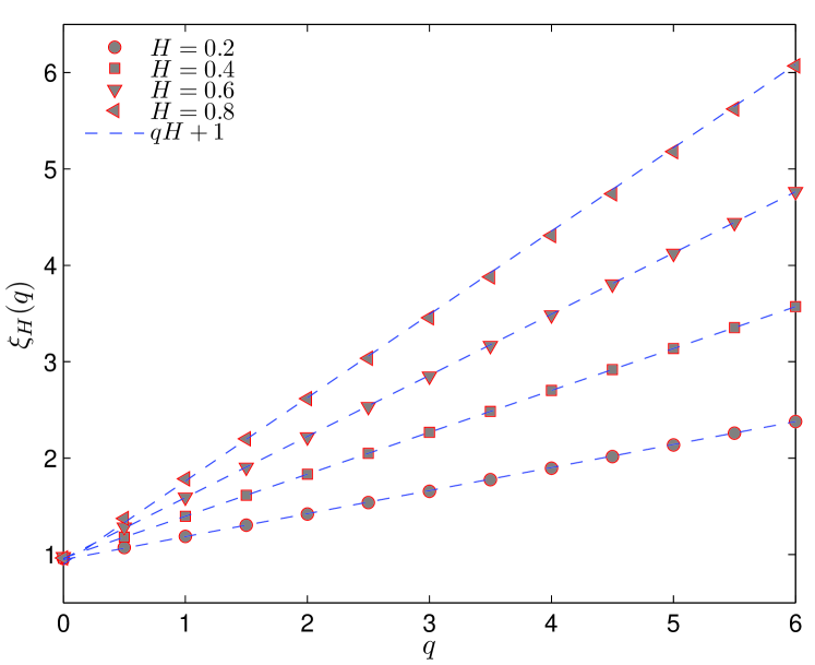
Figure 3: Scaling exponents $\xi(q)$ for fractional Brownian motion simulations with $H=0.2$, $0.4$, $0.6$ and $0.8$, respectively.

We first validate the new method by using fractional Brownian motion time series (fBm). They are characterized by the Hurst number $0\leq H\leq 1$, and it is well-known that $\zeta(q)=qH$, hence we expect $\xi(q)=1+qH$. We simulate 500 segments of length $2^{12}$ data points each, using a wavelet based algorithm [22], with different $H$ value from 0.2 to 0.8. The Hilbert transform is numerically estimated by using a FFT based method [23]. The scale invariance is perfectly respected as expected, this is not shown here, see ref.[21] for more detail on validations of the method with fBm simulation. We then represent the corresponding scaling exponents $\xi(q)$ for various value of $q$ from 0 to 6, for four values of $H$ ($H=0.2$, $0.4$, $0.6$ and $0.8$) in fig. 3. The perfect straight lines of equation $1+qH$ confirm the usefulness of the new method to estimate $\xi(q)$.

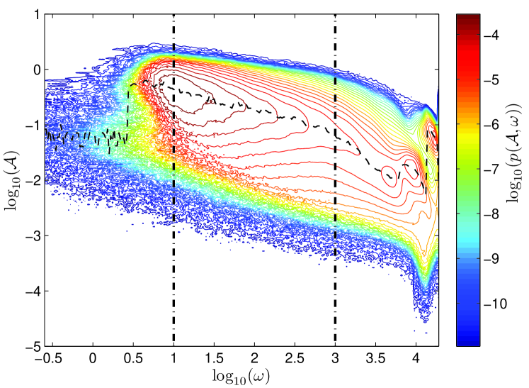
Figure 4: Representation of the joint pdf ${p}(\omega,\mathcal{A})$ (in log scale) of turbulent fluctuations in an amplitude-frequency space. The scaling range $10<\omega<1000\un{Hz}$ for frequencies is shown as vertical dotted lines. The dashed line shows the skeleton $\mathcal{A}_{\mathrm{s}}(\omega)$ of the joint pdf, which is the amplitude for which the conditional pdf $p(\mathcal{A}|\omega)$ is maximum.

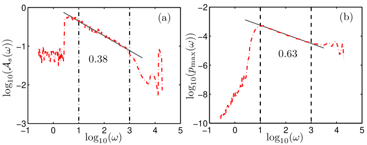
Figure 5: The skeleton of the joint pdf. (a) $\mathcal{A}_{\mathrm{s}}(\omega)$ in log-log plot. A power law behaviour is observed in the inertial subrange with scaling exponent 0.38, which is close to the Kolmogorov value 1/3. (b) $p_{\max}(\omega)$ in log-log plot. A power law behaviour is observed in the inertial subrange with scaling exponent 0.63. The vertical lines show the corresponding inertial subrange $10<\omega<1000\un{Hz}$.

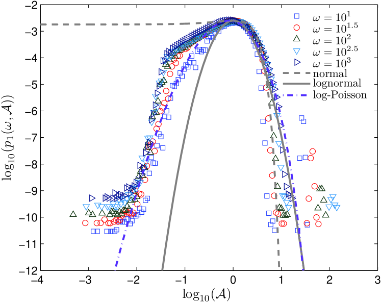
Figure 6: Representation of the rescaled conditional pdf $p_{1}(\mathcal{A},\omega)$ in the inertial range, for fixed values of $\omega=10$, $10^{1.5}$, $10^{2}$, $10^{2.5}$ and $10^{3}\un{Hz}$.

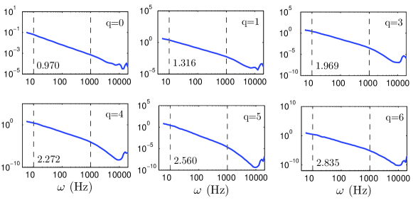
Figure 7: Representation of $\mathcal{L}_{q}(\omega)$, Hilbert spectral analysis of velocity intermittency, using different orders of moments (0, 1, 3, 4, 5 and 6). Power laws are observed on the range $10<\omega<1000\un{Hz}$ for all spectra. The value of the scaling exponent $\xi(q)$ is shown in each figure.

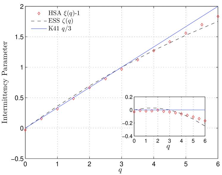
Figure 8: Comparison of the scaling exponents $\xi(q)-1$ (diamond) with the classical $\zeta(q)$ obtained from structure functions analysis with the ESS method (dash-dotted line) and K41 $q/3$ (solid line). The insert shows the departure from the K41 law.

We then consider turbulence intermittency properties using this approach. The EMD-HSA methodological framework provides a way to represent turbulent fluctuations in an amplitude-frequency space: the joint pdf ${p}(\omega,\mathcal{A})$ is shown in fig. 4. The inertial subrange for frequencies is shown as vertical dotted lines. This figure is the first 2D amplitude-frequency representation of the pdf of turbulent fluctuations; it can be seen graphically that the amplitudes decrease with increasing frequencies, with a scaling trend. We show in the same graph the skeleton $\mathcal{A}_{\mathrm{s}}(\omega)$ of the joint pdf which corresponds to the amplitude for which the conditional pdf $p(\mathcal{A}|\omega)$ is maximum:

$$\mathcal{A}_{\mathrm{s}}(\omega)=\mathcal{A}_{0}\,;\,p(\mathcal{A}_{0},\omega)=\max_{\mathcal{A}}\{p(\mathcal{A}|\omega)\}$$ (8)

We then reproduce the skeleton in fig. 5 in two different views: (a) $\mathcal{A}_{\mathrm{s}}(\omega)$ in log-log plot; (b) skeleton pdf $p_{\max}(\omega)=p(\mathcal{A}_{\mathrm{s}}(\omega),\omega)=\max_{\mathcal{A}}\{p(\mathcal{A}|\omega)\}$ in log-log plot. It is interesting to note that a power law behaviour is found for both representations

$$\mathcal{A}_{\mathrm{s}}(\omega)\sim\omega^{-\beta_{1}},\,\,p_{\max}(\omega)\sim\omega^{-\beta_{2}}$$ (9)

where $\beta_{1}\simeq 0.38$, and $\beta_{2}\simeq 0.63$. Dimensional analysis provides the non-intermittent Kolmogorov value $\beta_{1}=1/3$ and $\beta_{2}=2/3$. The difference with these theoretical value may be an effect of intermittency. We note that the value $\beta_{1}=0.38$ is comparable with the estimation of $\zeta(1)=0.37$ given by Ref. [24]. We plot in fig. 6 the rescaled pdf $p_{1}(\mathcal{A},\omega)=\omega^{\beta_{2}}p(\mathcal{A}/\omega^{\beta_{1}},\omega)$, for various fixed values of $\omega$. In case of monoscaling, these pdfs should superpose perfectly; here the plot is scattered, but nevertheless we note that the lack of superposition of these rescaled pdfs is a signature of intermittency. Moments of this pdf are less noisy as will be visible bellow. For comparison, we plot the normal distribution (dashed line), lognormal distribution (solid line) and log-Poisson distribution (dashed-dotted line) in the same figure. It seems that the log-Poisson distribution provides a better fit to the pdf than the lognormal distribution. We also characterize intermittency in the frequency space by considering marginal moments $\mathcal{L}_{q}(\omega)$. Figure 7 shows $\mathcal{L}_{q}(\omega)$, Hilbert spectral analysis of velocity intermittency, using different orders of moments (0, 1, 3, 4, 5 and 6). The moment of order 0 is the marginal pdf of the instantaneous frequency, see eq. (6). It is interesting to note that this pdf is extremely “wild”, having a behaviour close to $\mathcal{L}_{0}(\omega)\sim\omega^{-1}$, corresponding to a “sporadic” process whose probability density is not normalizable ($\int p(\omega)\,\upd\omega$ diverges). This result is only obtained when all modes are considered together; such pdf is not found for the frequency pdf of an individual mode. This property seems to be rather general: we observed such pdf for moment of order zero using several other time series: for example surf-zone turbulence data, fBm [21], river flow discharge data. Hence it does not seems to be linked to turbulence itself, but to be a main property of the HSA method, which still needs to be studied further. We observe the power laws in range $10<\omega<1000\un{Hz}$ for all order moments. The values of scaling exponents $\xi(q)$ are shown in each picture. This provides a way to estimate scaling exponents $\xi(q)$ for every order of moment $q\geq 0$ on a continuous range of scales in the frequency space.

Next, we compare scaling exponents $\xi(q)-1$ estimated by our new approach with the classical structure functions scaling exponent function $\zeta(q)$ estimated using the extended self similarity (ESS) method [25] in fig. 8. It can be seen that $\xi(q)-1$ is nonlinear and is close to $\zeta(q)$, but the departure from K41 law shows that the curvature is not the same: $\xi(q)$ seems less concave than $\zeta(q)$.

Here, we provide some comments on some issues of the EMD method. The main drawback of the EMD method is a lack of solid theoretical ground, since it is almost empirical [9]. It has been found experimentally that the method, especially for the HSA, is statistically stable with different stopping criteria [6]. Recently, Flandrin et al. have obtained new theoretical results on the EMD method [5, 26, 27]. However, more theoretical work is still needed to fully understand this method.

4 Conclusion

We have applied here empirical mode decomposition to analyze a high Reynolds number turbulent experimental time series. After decomposition, the original velocity time series is separated into several intrinsic modes. We showed that this method acts as an almost dyadic filter bank in the frequency domain, confirming previous results that have been obtained on Gaussian noise or fractional Gaussian noise. Comparing the Fourier spectrum of each mode, and the associated characteristic scale, we can interpret each mode according to the range to which it belongs. The first mode contains the smallest scale and the measurement noise; two modes are associated to dissipation scales, and many modes are associated to the inertial subrange corresponding to the turbulent energy cascade. The last modes correspond to the large scales associated to the coherent structures (energy-containing structures).

We have obtained a first 2D representation of the joint pdf $p(\omega,\mathcal{A})$. We observed a interesting power law behaviour with scaling exponent $\beta_{1}\simeq 0.38$ for the location of the joint pdf skeleton points. We also observed a power law behaviour with scaling exponent $\beta_{2}\simeq 0.63$ for the skeleton pdf $p_{\max}(\omega)$. It is also found that the log-Poisson distribution provides a better fit to the velocity pdf than the lognormal distribution. Then the intermittency information in multiscaling (multifractal) turbulent processes was extracted using the HSA framework. The scaling exponents in amplitude-frequency space ($\xi(q)-1$) are close to the ones in real space $\zeta(q)$, despite the quite different approaches used in both cases.

We have here extended the EMD-HSA approach in a quite natural way in order to consider intermittency. This provides a new time-frequency analysis for multifractal time series, that is likely to be applicable to other fields within the multifractal framework.

- [1] \NameHuang N. E., Shen Z., Long S. R., Wu M. C., Shih H. H., Zheng Q., Yen N., Tung C. C. Liu H. H. \REVIEWProc. R. Soc. London 4541998903.
- [2] \NameHuang N. E., Shen Z. Long S. R. \REVIEWAnnu. Rev. Fluid Mech. 311999417.
- [3] \NameWu Z. Huang N. E. \REVIEWProc. R. Soc. London 46020041597.
- [4] \NameFlandrin P., Rilling G. Gonçalvès P. \REVIEWIEEE Sig. Proc. Lett.112004112.
- [5] \NameFlandrin P. Gonçalvès P. \REVIEWInt. J. of Wavelets, Multires. and Info. Proc 22004477.
- [6] \NameHuang N. E., Wu M. L., Long S. R., Shen S. S. P., Qu W., Gloersen P. Fan K. L. \REVIEWProc. R. Soc. London 45920032317.
- [7] \NameCohen L. \BookTime-frequency analysis (Prentice Hall PTR Englewood Cliffs, NJ) 1995.
- [8] \NameLong S. R., Huang N. E., Tung C. C., Wu M. L., Lin R. Q., Mollo-Christensen E. Yuan Y. \REVIEWIEEE Geoscience and Remote Sensing Soc. Lett. 319956.
- [9] \NameHuang N. E. \BookHilbert-Huang Transform and Its Applications (World Scientific) 2005 Ch. 1. Introduction to the hilbert huang trasnform and its related mathmetical problems pp. 1–26.
- [10] \NameSu Z. Y., Wang C. C., Wu T., Wang Y. T. Tang F. C. \REVIEWPhysica A 3872008485.
- [11] \NameJánosi I. Müller R. \REVIEWPhys. Rev. E 712005056126.
- [12] \NameSolé J., Turiel A. Llebot J. \REVIEWNat. Hazards Earth Syst. Sci. 72007299.
- [13] \NameChen J., Xu Y. L. Zhang R. C. \REVIEWJ. Wind Eng. Ind. Aerodyn. 922004805.
- [14] \NameLoutridis S. J. \REVIEWAppl. Acoust. 6620051399.
- [15] \NameKang H., Chester S. Meneveau C. \REVIEWJ. Fluid Mech. 4802003129.
- [16] \NameFrisch U. \BookTurbulence: the legacy of AN Kolmogorov (Cambridge University Press) 1995.
- [17] \NameSchertzer D. Lovejoy S. \REVIEWJ. Geophys. Res. 9219879693.
- [18] \NameSeuront L., Schmitt F. G., Lagadeuc Y., Schertzer D. Lovejoy S. \REVIEWJ. Plankton Res. 211999877.
- [19] \NameAshkenazy Y., Hausdorff M. J., Ivanov P. Ch. Stanley H. E. \REVIEWPhysica A 3162002662.
- [20] \NameSchmitt F. G., Schertzer D. Lovejoy S. \REVIEWAppl. Stoch. Models and Data Anal. 15199929.
- [21] \NameHuang Y. X., Schmitt F. G., Lu Z. M. Liu Y. L. Analyse de l’invariance d’échelle de séries temporelles par la décomposition modale empirique et l’analyse spectrale de Hilbert \REVIEWTraitement du Signal2008submitted.
- [22] \NameAbry P. Sellan F. \REVIEWAppl. Comput. Harmon. Anal. 31996377.
- [23] \NameMarple J. L. \REVIEWIEEE Trans. Signal Process 4719992600.
- [24] \Namevan de Water, W. Herwijer, J. A. \REVIEWJ. Fluid Mech. 38719993.
- [25] \NameBenzi R., Ciliberto S., Tripiccione R., Baudet C., Massaioli F. Succi S. \REVIEWPhys. Rev. E 48199329.
- [26] \NameRilling, G. Flandrin, P. \REVIEWIEEE, ICASSP 2006 32006444.
- [27] \NameRilling, G. Flandrin, P. \REVIEWIEEE Trans. Signal Process 56200885.