Lagrangian Cascade in Three-Dimensional Homogeneous and Isotropic Turbulence

Abstract

In this work, the scaling statistics of the dissipation along Lagrangian trajectories are investigated by using fluid tracer particles obtained from a high resolution direct numerical simulation with $Re_{\lambda}=400$. Both the energy dissipation rate $\epsilon$ and the local time averaged $\epsilon_{\tau}$ agree rather well with the lognormal distribution hypothesis. Several statistics are then examined. It is found that the autocorrelation function $\rho(\tau)$ of $\ln(\epsilon(t))$ and variance $\sigma^{2}(\tau)$ of $\ln(\epsilon_{\tau}(t))$ obey a log-law with scaling exponent $\beta^{\prime}{}=\beta=0.30$ compatible with the intermittency parameter $\mu=0.30$. The $q$th-order moment of $\epsilon_{\tau}$ has a clear power-law on the inertial range $10<\tau/\tau_{\eta}<100$. The measured scaling exponent $K_{L}(q)$ agrees remarkably with $q-\zeta_{L}(2q)$ where $\zeta_{L}(2q)$ is the scaling exponent estimated using the Hilbert methodology. All these results suggest that the dissipation along Lagrangian trajectories could be modelled by a multiplicative cascade.

1 Introduction

Turbulent flows are complex and multiscale and are characterized by eddy motions of different spatial sizes with different time scales (Frisch, 1995; Pope, 2000; Tsinober, 2009). This has been described by Kolmogorov’s scaling theory of turbulence in 1941. The scaling behavior of the Eulerian velocity field has been studied in details to quantify the intermittent nature of turbulence for large Reynolds numbers and homogeneous turbulence (Sreenivasan & Antonia, 1997; Frisch, 1995). Here we consider the Lagrangian frame, in which the fluid particle is tracked experimentally or numerically (Mordant et al., 2002; Yeung, 2002; Chevillard et al., 2003; Biferale et al., 2004; Xu et al., 2006a; Chevillard & Meneveau, 2006; Toschi & Bodenschatz, 2009; Meneveau, 2011). Fluid particles are fluctuating over different time scales with a power-law behavior in the inertial range, e.g., $\tau_{\eta}\ll\tau\ll T_{L}$, in which $\tau_{\eta}$ is the Kolmogorov time scale, and $T_{L}$ is the Lagrangian integral time scale. Conventionally, multiscale statistics are characterized by using the Lagrangian structure-functions (LSFs), i.e., $S_{L}^{q}(\tau)=\langle|\Delta_{\tau}u(t)|^{q}\rangle\sim\epsilon^{q/2}\tau^{q/2}$ in which $\Delta_{\tau}u(t)=u(t+\tau)-u(t)$ is the Lagrangian velocity increment, and $\tau$ is the separation time scale and is lying in the inertial range. Recently, Huang et al. (2013) showed a clear Lagrangian inertial range on the frequency range $0.01<\omega\tau_{\eta}<0.1$ (resp. $10<\tau/\tau_{\eta}<100$) and retrieved the scaling exponent $\zeta_{L}(q)$ by using a Hilbert-based methodology. The measured scaling exponents $\zeta_{L}(q)$ are nonlinear and concave, showing that intermittency corrections are indeed relevant for Lagrangian turbulence (Borgas, 1993; Chevillard et al., 2003; Biferale et al., 2004; Xu et al., 2006b). Using a high-resolution Lagrangian turbulence database, we can now verify the scaling relations associated with the Kolmogorov refined similarity hypothesis (RSH).

2 Refined Similarity Hypothesis

Let us recall some main ingredients of the Lagrangian version of the Kolmogorov’s refined similarity hypothesis (LRSH), in which the energy dissipation rate $\epsilon=2\nu S_{ij}S_{ij}$ is involved. Here $S_{ij}=1/2(\partial u_{i}/\partial x_{j}+\partial u_{j}/\partial x_{i})$ is the velocity strain rate tensor along a Lagrangian trajectory. A local time averaged of the energy dissipation rate along a Lagrangian trajectory is defined as, i.e.,

$$\epsilon_{\tau}(t)=\frac{1}{\tau}\int_{0\leq t^{\prime}{}\leq\tau}\epsilon(t+t^{\prime}{})\mathrm{\,d}t^{\prime}{},\,X_{\tau}(t)=\ln(\epsilon_{\tau}(t))$$ (1)

where $X_{\tau}(t)$ is the logarithm of the dissipation. Kolmogorov’s RSH (1962) has been written in the Eulerian frame. The Lagrangian analogy assumes that, in the inertial range, the variance of $X_{\tau}(t)$ has a logarithmic decrease, i.e.,

$$\sigma^{2}(\tau)=A-\beta\ln(\tau)$$ (2)

in which $\sigma^{2}$ stands for the variance of $X_{\tau}$, $\beta$ is a universal constant and $A$ might depend on the flow (Kolmogorov, 1962). A $q$th-order moment of $\epsilon_{\tau}$ is expected to have a power-law behavior in the inertial range, i.e.,

$$M_{q}(\tau)=\langle\epsilon_{\tau}^{q}\rangle\sim\tau^{-K_{L}(q)}$$ (3)

This relation can be completed by a logarithmic decrease of the autocorrelation function of $X(t)=\ln(\epsilon(t))$ associated to multifractal cascades (Arneodo et al., 1998), i.e.,

$$\rho(\tau)=\langle\tilde{X}(t)\tilde{X}(t+\tau)\rangle=A^{\prime}{}-\beta^{\prime}{}\ln(\tau)$$ (4)

in which $\tilde{X}=X-\langle X\rangle$. For a lognormal cascade, we expect $\mu=K_{L}(2)=\beta=\beta^{\prime}{}$, in which $\mu$ is the intermittency parameter (Schmitt, 2003). On the other hand, one expects also a power-law behavior for the $q$th-order LSF, $S_{q}^{L}(\tau)\sim\tau^{\zeta(q)}$. The LRSH assumes a relationship between these two quantities, i.e.,

$$S_{L}^{q}(\tau)\sim\langle\epsilon_{\tau}^{q/2}\rangle\tau^{q/2}\sim\tau^{q/2-K_{L}(q/2)}$$ (5)

leading to a relation between scaling exponents, i.e.,

$$\zeta_{L}(q)=q/2-K_{L}(q/2)$$ (6)

Let us note that this scaling relation (Eq. 6) can be found for non-lognormal cascades so that the original Kolmogorov assumption of lognormality is not included in the RSH. The original RSH in the Eulerian frame has been very well verified (Stolovitzky et al., 1992; Stolovitzky & Sreenivasan, 1994; Chen et al., 1997; Praskovsky et al., 1997). However, only few works have tested the RSH in Lagrangian frame (Chevillard et al., 2003; Yu & Meneveau, 2010; Benzi et al., 2009; Sawford & Yeung, 2011; Homann et al., 2011). For example, Chevillard et al. (2003) proposed a multifractal formula to describe the Lagrangian velocity increments. It is found that the left part of the measured singularity spectrum $D(h)$ agrees well with both the lognormal model and the log-Poisson model. Yu & Meneveau (2010) investigated the Lagrangian time correlation function $\rho(\tau)$ for both Lagrangian strain- and rotation-rate tensors. They found that the correlation function $\rho(\tau)$ depends on the spatial location of particles released. Benzi et al. (2009) tested the LRSH along Lagrangian trajectories. They showed that the LRSH is well verified by making Extended Self-Similarity plots. Homann et al. (2011) studied a conditional Lagrangian increment statistics. They found that the intermittency is significantly reduced when the LSF is conditioned on the energy dissipation rate or similar quantities (e.g., square of vorticity). A similar result has been shown for the Eulerian velocity structure-function: it is found that if one removes strong dissipation events, the corresponding scaling exponent is then approaching the Kolmogorov’s 1941 ones without intermittent correction (Kholmyansky & Tsinober, 2009). Note that in all these studies, the relation 6 was not directly tested.

We would like to provide a comment on the LSF. It has been shown that due to the influence of large scale motions, known as infrared effect, and to the contamination of small scales, known as ultraviolet effect, the classical LSF mixes the large and small scales information (Huang et al., 2013). Therefore, without the help of ESS, the LSF can not identify the correct scaling behavior of the Lagrangian velocity (Mordant et al., 2002; Xu et al., 2006a; Sawford & Yeung, 2011; Falkovich et al., 2012). With the help of a fully adaptive method, namely Hilbert-Huang transform, a clear inertial range can be found (Huang et al., 2013). In this paper, the LRSH is verified by considering Eqs. 2, 3, 4 and 6, where the scaling exponents for the Lagrangian velocity are extracted by using a Hilbert-based method.

3 Numerical Validation

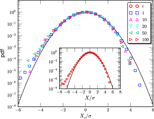
Figure 1: (Color online) Measured pdf of the $X=\ln(\epsilon)$ and local averaged $X_{\tau}=\ln(\epsilon_{\tau})$ for several time scales in both dissipative ($\tau/\tau_{\eta}<10$) and inertial ($\tau/\tau_{\eta}\geq 10$) ranges. For comparison, the normal distribution is illustrated by a solid line. Graphically, except for values with $|X_{\tau}|>4\sigma$, the measured pdfs agree well with the lognormal distribution. Note that for display clarity, the measured pdf has been centered and vertically shifted by plotting $p(X_{\tau})=p_{\tau}(X_{\tau})/p_{\max}(\tau)$, in which $p_{\max}(\tau)=\max_{X_{\tau}}\left\{p_{\tau}(X_{\tau})\right\}$.

Figure 2: (Color online) Measured max value of pdfs, $p_{\max}(\tau)-p_{\max}(0)$, in which the inertial range $10\leq\tau/\tau_{\eta}\leq 100$ is illustrated by a dashed line. The upper inset shows the measured $p_{\max}(\tau)$, in which the solid line is the power-law fitting. The lower inset shows the compensated curve $\left(p_{\max}(\tau)-p_{\max}(0)\right)\tau^{-0.81}$. A power-law behavior is observed in the inertial range $10<\tau/\tau_{\eta}<100$ with a scaling exponent $\alpha=0.81\pm 0.03$. The statistical error of $\alpha$ is the difference between the scaling exponent fitted on the first and second half of the scaling range (in log scale).

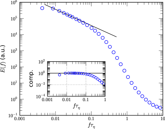
Figure 3: (Color online) Measured Fourier power spectrum of $\ln(\epsilon)$. A power law behavior is observed on the range $0.01<f\tau_{\eta}<0.06$ with a scaling exponent $1.06\pm 0.13$. The inset shows the compensated curve with fitted parameters.

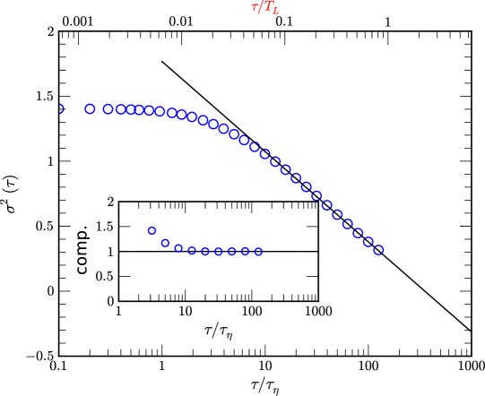
Figure 4: (Color online) Measured variance $\sigma^{2}(\tau)$ ($\ocircle$) of $\ln(\epsilon_{\tau})$ ($\ocircle$). A log-law is observed with a scaling exponent $\beta=0.30\pm 0.01$ on the range $10<\tau/\tau_{\eta}<100$. The inset shows the compensated curve with fitted parameters to emphasize the log-law. The statistical error of $\beta$ is estimated as in Fig. 2.

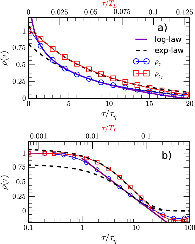
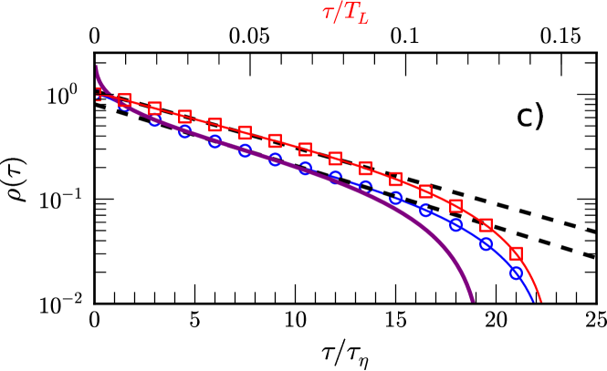
Figure 5: (Color online) Measured autocorrelation function $\rho(\tau)$ for the logarithm of the energy dissipation rate $\epsilon$ ($\ocircle$) and pseudo-dissipation $\epsilon_{T}$ ($\square$). a) lin-lin plot, in which the dashed line and solid line are respectively exponential and logarithmic fitting. b) semilogx plot and c) semilogy plot. An exponential law is observed respectively on the range $3<\tau/\tau_{\eta}<15$ (resp. $0.019<\tau/T_{L}<0.097$) for $\epsilon$ and on the range $0<\tau/\tau_{\eta}<15$ (resp. $0<\tau/T_{L}<0.097$) for $\epsilon_{T}$. Log-law fitting is observed on the range $1<\tau/\tau_{\eta}<15$ (resp. $0.0065<\tau/T_{L}<0.097$) with a scaling exponent $\beta^{\prime}{}=0.30\pm 0.01$ for the full dissipation $\epsilon$, verifying Eq. 4.

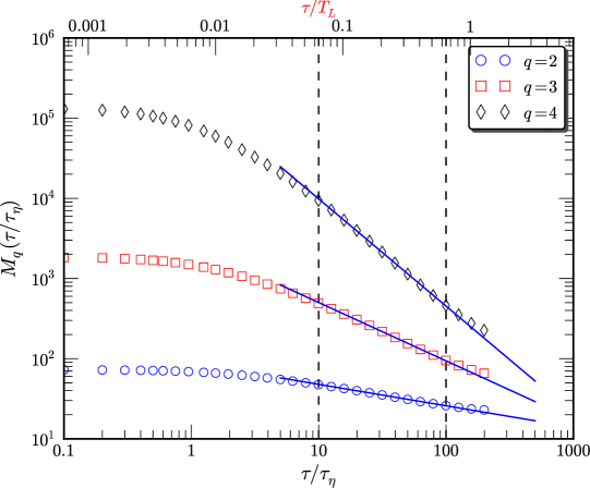
Figure 6: (Color online) Measured $M_{q}(t/\tau)$ for $q=2,3$ and $4$, in which the inertial range $10\leq\tau/\tau_{\eta}\leq 100$ is indicated by a dashed vertical line. Power law behavior is observed on this inertial range for all moments we considered here. The scaling exponents $K_{L}(q)$ are then estimated on this inertial range.

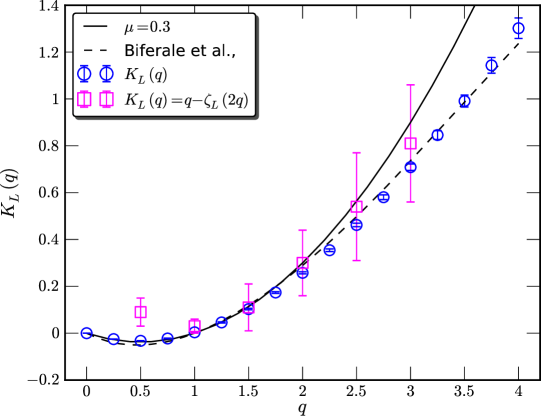
Figure 7: (Color online) Measured $K_{L}(q)$ ($\ocircle$) and $q-\zeta_{L}(2q)$ ($\square$) provided by a Hilbert method. For comparison, the curve predicted by the lognormal model with an intermittent parameter $\mu=0.30$ (solid line) and the log-Poisson based multifractal model (dashed line) are also shown. The errorbar is the difference between the scaling exponent fitted on the first and second half of the inertial range (in log scale).

The dataset considered here is composed by Lagrangian velocity trajectories in a homogeneous and isotropic turbulent flow obtained from a $2048^{3}$ DNS simulation with a Reynolds number $Re_{\lambda}=400$. We recall briefly some key parameters of this database. There are $\sim 2\cdot 10^{5}$ fluid tracer trajectories, each composed by $N=4720$ time sampling saved every $0.1\tau_{\eta}$ time units, in which $\tau_{\eta}$ is the Kolmogorov time scale. Hence, we can access time scales in the range $0.1<\tau/\tau_{\eta}<236$. The integral time scale $T_{L}$ is estimated by using the well-known Kolmogorov scaling relation as, i.e., $T_{L}/\tau_{\eta}=Re^{1/2}\simeq 155$, in which $Re=\frac{3}{20}Re_{\lambda}^{2}$ (Pope, 2000). The full energy dissipation rate $\epsilon(t)$ is retrieved from this database along the Lagrangian trajectories. Previously, an inertial range $0.01<\omega\tau_{\eta}<0.1$ (resp. $10<\tau/\tau_{\eta}<100$ or $0.065<\tau/T_{L}<0.65$) has been reported for this database by using a Hilbert-based methodology (Huang et al., 2013). We therefore focus on this inertial range in the following analysis. The details of this database can been found in Benzi et al. (2009).

Figure 1 shows the measured pdf $p(X)$ and $p_{\tau}(X_{\tau})$ for time scales in the dissipative ($\tau/\tau_{\eta}<10$) and inertial ($\tau/\tau_{\eta}>10$) ranges. For display clarity, the measured $p_{\tau}(X_{\tau})$ have been centered and vertically shifted by taking $p(X_{\tau})=p_{\tau}(X_{\tau})/p_{\max}(\tau)$, in which $p_{\max}(\tau)=\max_{X_{\tau}}\left\{p_{\tau}(X_{\tau})\right\}$. For comparison, the Gaussian distribution is illustrated as a solid line. Graphically, the measured pdf is slightly deviating from the Gaussian distribution when $|X|>4\sigma$. This confirms that the lognormal assumption for the energy dissipation rate approximately holds also in the Lagrangian frame at least for the central part of the pdf for $|X|<4\sigma$.

Figure 2 shows the measured maximum value of the pdf $p_{\max}({\tau})-p_{\max}(0)$, in which the inertial range $10<\tau/\tau_{\eta}<100$ is indicated by a dashed line. Here $p_{\max}(0)$ is for the original energy dissipation rate. A power-law behavior is observed on the inertial range, i.e.,

$$p_{\max}({\tau})-p_{\max}(0)\sim\tau^{\alpha}$$ (7)

with a measured scaling exponent $\alpha=0.81\pm 0.03$. Note that the statistical error of $\alpha$ is the difference between the scaling exponent fitted on the first and second half of the inertial range (in log scale). In the upper inset, we show the measured $p_{\max}(\tau)$, in which the solid line is the power-law fitting. In the lower inset we show the compensated curve $\left(p_{\max}({\tau})-p_{\max}(0)\right)\tau^{-0.81}$ to emphasize the observed power-law. A plateau is observed in the inertial range. To our knowledge, it is the first time that this pdf scaling relation is found. We have no interpretation presently for this relation and for the value of its exponent $\alpha$.

Figure 3 shows the measured Fourier power spectrum $X=\ln(\epsilon)$. A power-law behavior is observed in the range $0.01<f\tau_{\eta}<0.06$ with a scaling exponent $1.06\pm 0.13$. The inset shows a compensated curve by using the fitted parameters to emphasize the observed power-law behavior. Figure 4 shows the measured variance $\sigma^{2}(\tau)$ of $\ln(\epsilon_{\tau}(t))$ ($\ocircle$). A log-law is observed for $\sigma^{2}(\tau)$ respectively on the range $10<\tau/\tau_{\eta}<100$ with a scaling exponent $\beta=0.30\pm 0.01$. The inset shows the corresponding compensated curve to emphasize the observed log-law. Eq. 2 is thus verified. Note that the $1/f$ type Fourier power spectrum is a consequence of a multiplicative cascade. Hence, this result is consistent with the logarithmic decay of the variance observed here. We also note that Pope & Chen (1990) have proposed an Ornstein-Uhlenbeck process for the dissipation field, which would predict a Lorentzian (or Cauchy) spectrum, i.e. a $f^{-2}$ decreasing. Here the observed $1/f$ spectrum does not support the Ornstein-Uhlenbeck proposal.

Figure 5 shows the measured autocorrelation function $\rho(\tau)$ for both the logarithm of the energy dissipation rate $\epsilon$ ($\ocircle$) and pseudo-dissipation $\epsilon_{T}=\nu\frac{\partial u_{i}}{\partial x_{j}}\frac{\partial u_{i}}{\partial x_{j}}$ ($\square$): a) lin-lin plot, b) semilogx plot and c) semilogy plot, respectively. The measured $\rho_{\epsilon}(\tau)$ and $\rho_{\epsilon_{T}}(\tau)$ cross zero at $\tau/\tau_{\eta}\simeq 23$. This is consistent with the observation in Ref. Pope (1990). We test the log-law, i.e., Eq. 4 first, see Fig. 5 b). A log-law is observed for the dissipation $\epsilon$ on the range $1<\tau/\tau_{\eta}<15$ ($0.0065<\tau/T_{L}<0.097)$ with a scaling exponent $\beta^{\prime}{}=0.30\pm 0.01$. However, the log-law is less pronounced for the pseudo-dissipation. The log-law is illustrated by a thick solid line in Fig. 5. We note that Pope & Chen (1990) observed an exponential decay of $\rho(\tau)$. Figure 5 c) shows the measured $\rho(\tau)$ in semilogy plot. An exponential law is observed respectively on the range $3<\tau/\tau_{\eta}<15$ ($0.019<\tau/T_{L}<0.097$) for $\epsilon$ and $0<\tau/\tau_{\eta}<15$ ($0<\tau/T_{L}<0.097$) for $\epsilon_{T}$. The exponential law is represented by a dashed line in Fig. 5. Moreover, the exponential law of pseudo dissipation is more pronounced than the one of full dissipation. Visually, it is difficult to make a distinction between logarithmic and exponential laws. However, we note that an exponential decay as found by Pope & Chen (1990) is not compatible with the intermittency framework for Lagrangian statistics, which is now well accepted (Chevillard et al., 2003; Biferale et al., 2004). Despite the scaling range, Eq. 4 is verified. Note that the autocorrelation function can be related to the Fourier power spectrum via $\rho(\tau)=\int_{0}^{+\infty}E(f)\cos(2\pi f\tau)\mathrm{\,d}f$, in which $E(f)$ is the Fourier power spectrum of $X$. Therefore, except for $f=(n+1/2)/2\tau$, $n=0,1,2,\cdots$, all Fourier modes contribute to $\rho(\tau)$, indicating a mixing of large- and small-scale information. This could be one reason for the shift of the scaling range. A similar phenomenon is observed for the structure-function, which could be understood as a finite size effect of the range of the power-law, known as infrared effect (large-scale motions) and ultraviolet effect (small-scale motions) (Huang et al., 2010, 2013).

The intermittency parameter $\mu=2-\zeta_{L}(4)=0.30\pm 0.14$ provided by the Hilbert method (Huang et al., 2013) is consistent with the scaling exponents $\beta$ and $\beta^{\prime}{}$ we obtained here. Let us note here that the covariance log-relation was not an hypothesis of Kolmogorov, and is a relation which is different from Eq. 2. However there are some relations between them: for a lognormal multiplicative cascade with intermittency parameter $\mu=K_{L}(2)$, it can be shown that the covariance of $X$ should have a log-law with parameter $\beta^{\prime}{}=\mu$ (Kahane, 1985). Kolmogorov’s hypothesis for the variance of $X_{\tau}$ is also a consequence of the cascade and its parameter is $\beta=\mu$. Here we find $\mu=0.30$ and the values for the slopes of the covariance and variance rescaling, are fully compatible with this value of the intermittency parameter. We also note that the direct estimation of the intermittency parameter from the Eulerian structure function is $\mu_{E}=2-\zeta(6)=0.34\pm 0.03$ (not shown here). It is also compatible with the value we obtain for Lagrangian fluctuations. Furthermore, when the covariance has a logarithmic decay, the Fourier power spectrum has a $-1$ scaling, also found here. All these results are consistent, and confirm that the dissipation in the Lagrangian frame can be described by a multiplicative cascade.

Figure 6 shows the measured $M_{q}(\tau)$ for $q=2,3$ and $4$. Power-law behavior is observed for all moments on the inertial range $10<\tau/\tau_{\eta}<100$. The scaling exponent $K_{L}(q)$ is then estimated on this range. Figure 7 shows the measured $K_{L}(q)$ ($\ocircle$) on the range $0<q<4$. The errorbar is the difference between the scaling exponent fitted on the first and second half of the inertial range (in log scale). For comparison, the $K_{L}(q)=q-\zeta_{L}(2q)$ ($\square$) provided by the Hilbert-based methodology is also shown. We estimated $\zeta_{L}(q)$ up to $q=6$ by using the Hilbert-based method (Huang et al., 2013). The corresponding $q$ for $K_{L}(q)$ is $3$. The definition of the errorbar is the same as the one for $K_{L}(q)$. The $K_{L}(q)$ provided by Biferale et al. (2004) log-Poisson based multifractal model and by the lognormal model with the intermittency parameter $\mu=0.30$ are respectively shown as a dashed and solid line. For $q\leq 3$, all symbols collapse, showing the validity of the scaling relation of Eq.6 predicted by the LRSH. For $q>3$, the measured $K_{L}(q)$ deviates from the lognormal model since the high-order $M_{q}(\tau)$ corresponds the statistics of the tail of the pdf and we observed deviations from the Gaussian distribution when $X>4\sigma$.

4 Conclusion

In summary, the scaling statistics of the energy dissipation along the Lagrangian trajectory is investigated by using fluid tracer particles obtained from a high resolution direct numerical simulation with $Re_{\lambda}=400$. Both the energy dissipation rate $\epsilon$ and the local time averaged $\epsilon_{\tau}$ agree reasonably with the lognormal distribution hypothesis. The measured $p_{\max}(\tau)-p_{\max}(0)$ (maximum value of a pdf) obeys a power law with a scaling exponent $0.81$, a result for which we have no theoretical explanation. Several statistics of the energy dissipation are then examined. It is found that the autocorrelation function $\rho(\tau)$ of $\ln(\epsilon(t))$ and variance $\sigma_{\tau}^{2}$ of $\ln(\epsilon_{\tau})$ obey log-laws with scaling exponents compatible with the intermittency parameter $\mu=0.30$ as expected for multiplicative cascades. These results show that the dissipation along Lagrangian trajectories can be modelled by multiplicative cascades. The $q$th-order moment of $\epsilon_{\tau}$ has a clear power-law on the inertial range. The LRSH assumptions Eqs. 2 and 3, and scaling relation 6 are then verified.