Unitarity in a Lorentz symmetry breaking model with higher-order operators

Abstract

We analyze the unitarity of a modified QED with higher-order terms that violate Lorentz symmetry. We make an explicit calculation to verify unitarity at the one-loop level. As expected we find negative norm-states that could in principle lead to a violation of unitarity. However, we show that these states become massive in Euclidean space and do not contribute to the discontinuity.

I Introduction

At energy scales at the Planck mass, $m_{\text{Pl}}\approx 10^{19}~{}\text{GeV}$, gravitational forces become as strong as the electroweak forces. We expect that at experiments at the electroweak scale, given by the Z-boson mass, $m_{Z}\approx 91~{}\text{GeV}$, gravitational effects are suppressed by a factor $m_{Z}/m_{\text{Pl}}\approx 10^{-17}$. Nevertheless, gravitational effects of elementary particles could be observable at currently available energy scales Foam . One interesting class of these Planck-mass suppressed effects violate Lorentz invariance. This possibility has been widely explored in several contexts, such as in modified dispersion relations MDR , loop quantum gravity LQG , and string theory Strings ; Strings1 .

In an effective approach, Lorentz-invariance-violating terms may be imposed at the Lagrangian level. In Ref. SME the possible Lorentz-violating and renormalizable operators were classified. The principal idea is to impose gauge-invariant terms, involving non-Lorentz-invariant tensors with Planck-mass suppressed couplings. In this way, Lorentz invariance is explicitly broken, but the effective terms may originate from a spontaneously broken gravitational theory SLSB .

Recently the same idea has been extended to consider higher-order operators Myers-Pospelov ; higher-derivative2 ; SME-nonminimal . They also have been considered to solve the hierarchy problem in the standard model Higgs , regularization Regulator , and radiative corrections Radiative ; Reyes ; Mariz . In particular, in Ref. Myers-Pospelov the modifications of the dispersion relations originating from the modified kinetic terms of the Lagrangian with respect to scalars, fermions, and vector particles have been studied. From a comparison to astrophysical experiments, limits on the new couplings have been derived MP_Limits .

A possible drawback of the higher-order modifications of the kinetic terms is, that negative-norm states can appear PU ; Lee-Wick . These states correspond to massive modes of the photon field and could in principle violate unitarity. Therefore it appears quite essential to verify explicitly that unitarity is preserved Schrek . In previous works, it has been shown for Lorentz-violating modifications of photons Unitarity that in Bhabha scattering at the tree level unitarity is fulfilled. Here we want to proceed and show that unitarity is conserved in modified quantum electrodynamics at the one-loop level.

II The modified photon sector

We will consider the modified QED Lagrangian Myers-Pospelov

$$\mathcal{L}=\bar{\psi}(\hbox{{$\partial$}\hbox to0.0pt{\hss$/$}}-m)\psi-\frac{1}{4}F^{\mu\nu}F_{\mu\nu}-\frac{\xi}{2m_{\text{Pl}}}n_{\mu}\epsilon^{\mu\nu\lambda\sigma}A_{\nu}(n\cdot\partial)^{2}F_{\lambda\sigma}\;,$$ (1)

where $n$ is a noninvariant four-vector defining a preferred reference frame, $m_{\text{Pl}}$ is the Planck mass, and $\xi$ is a dimensionless coupling parameter. Obviously the modification term is a gauge-invariant dimension-five operator which is Planck-mass suppressed.

The equations of motion derived from the Lagrangian (1) read

$$\partial_{\mu}F^{\mu\nu}+g\epsilon^{\nu\alpha\lambda\sigma}n_{\alpha}(n\cdot\partial)^{2}F_{\lambda\sigma}=4\pi j^{\nu}\;,$$ (2)

where we have introduced a source $j^{\nu}$ and defined $g=\xi/m_{\text{Pl}}$. In addition we have to impose a gauge fixing, where we choose the axial gauge Andrianov ,

$$\partial_{\mu}A^{\mu}=0\;,\quad n_{\mu}A^{\mu}=0\;.$$ (3)

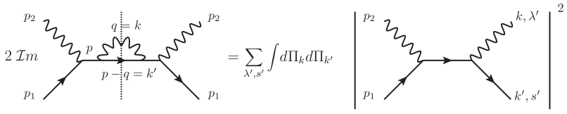
Figure 1: The optical theorem for a one-loop forward Compton scattering amplitude. The integrals $\int d\Pi_{k}d\Pi_{k^{\prime}}$ denote the phase-space integration over the final-state momenta.

In order to verify unitarity, we shall first derive the modified photon propagator originating from Eq. (1). To this end we write the equation of motion in the form

$$M^{\nu\sigma}A_{\sigma}(x)=4\pi j^{\nu},$$ (4)

where we have defined the operator $M^{\nu\sigma}=\eta^{\nu\sigma}\Box+2g\epsilon^{\nu\mu\alpha\sigma}n_{\mu}(n\cdot\partial)^{2}\partial_{\alpha}$. In order to construct the modified polarization vectors of the photon field, let us, following closely Ref. Andrianov , introduce the projectors onto the plane, transverse to both directions, $k$ and $n$,

$$e^{\mu\nu}=\eta^{\mu\nu}-\frac{(n\cdot k)}{D}(n^{\mu}k^{\nu}+n^{\nu}k^{\mu})+\frac{k^{2}}{D}n^{\mu}n^{\nu}\\ +\frac{n^{2}}{D}k^{\mu}k^{\nu}\;,$$ (5)

with $D=(n\cdot k)^{2}-n^{2}k^{2}$. We easily verify that indeed $k_{\mu}e^{\mu\nu}=n_{\mu}e^{\mu\nu}=0$ as well as $e^{\mu}_{\alpha}e^{\alpha\nu}=e^{\mu\nu}$. By means of these projectors we can construct two linear polarization vectors $e^{(1)}$ and $e^{(2)}$ respecting

$$e_{\mu\nu}=-\sum_{a=1,2}e_{\mu}^{(a)}e_{\nu}^{(a)}\;,\quad\eta^{\mu\nu}e_{\mu}^{(a)}e_{\nu}^{(b)}=-\delta^{ab}\;.$$ (6)

By these linear polarization vectors, modified circular polarization vectors are constructed,

$$\varepsilon_{\mu}(k,\lambda)=\frac{1}{2}\big{(}e_{\mu}^{(1)}+\lambda i\;e_{\mu}^{(2)}\big{)}\;,\\$$ (7)

with $\lambda=\pm 1$ corresponding to left and right polarizations, respectively. We can see, that the tensor

$$P^{(\lambda)}_{\mu\nu}=-\varepsilon_{\mu}(k,\lambda)\varepsilon^{*}_{\nu}(k,\lambda)\;,$$ (8)

acts as a projector onto the circular vectors,

$$\varepsilon_{\mu}(k,\lambda)=P_{\mu\nu}^{(\lambda)}e^{\nu(1)}\;.$$ (9)

Eventually, we end up with a modified dispersion relation

$$G=(k^{2})^{2}-4g^{2}(n\cdot k)^{4}\left((n\cdot k)^{2}-n^{2}k^{2}\right)=0\;,$$ (10)

and from the inverse of Eq. (4) we arrive at the modified photon propagator in the axial gauge,

$$G_{\mu\nu}(k)=-\sum_{\lambda}\frac{P^{(\lambda)}_{\mu\nu}(k)}{k^{2}+2g\lambda(k\cdot n)^{2}\sqrt{D}}\;.$$ (11)

III Unitarity

With the preparations in the previous section we may now compute discontinuities of amplitudes involving the modified Lorentz-violating Lagrangian (1). Let us first focus on the forward Compton scattering at the one-loop order with the corresponding Cutkosky cutting rules Cut , shown in Fig. 1. The imaginary part of the forward Compton scattering amplitude originates from the discontinuities of the propagators in the loop – along the cut on the left-hand side of Fig. 1. With respect to the Lagrangian (1) we now have to deal with a modified photon propagator (11) as well as modified photon polarization vectors (7). Following the optical theorem, unitarity of this diagram requires that 2 times the imaginary part of the forward scattering diagram $e^{-}(p_{1})+\gamma(p_{2})\rightarrow e^{-}(p_{1})+\gamma(p_{2})$ with the indicated loop is equal to the tree-level production cross section of photon plus electron, summed over the two final physical polarization states (respectively spin states) and integrated over the final-state phase space. This identity is a direct consequence of the unitarity of the S-matrix. In contrast to ordinary QED, here the modified photon propagator as well as the modified polarization vectors of the photons change the calculation of the loop amplitude and in principle could show a violation of unitarity.

Nevertheless, we shall verify, that the left-hand side and the right-hand side of the diagrams shown in Fig. 1 are equal, and therefore they do fulfill unitarity.

The right-hand side can immediately be written down as

$$\sum_{\lambda^{\prime},s^{\prime}}\int\frac{d^{3}k}{(2\pi)^{3}2k_{0}}\frac{d^{3}k^{\prime}}{(2\pi)^{3}2k^{\prime}_{0}}\left|\mathcal{M}\right|^{2}\delta^{(4)}(k+k^{\prime}-p_{1}-p_{2})(2\pi)^{4}\;,$$ (12)

with the matrix element

$$\mathcal{M}=-ie^{2}\frac{1}{(p^{2}-m^{2})}\varepsilon^{*}_{\mu}(k,\lambda^{\prime})\bar{u}(k^{\prime},s^{\prime})\gamma^{\mu}(\hbox{{$p$}\hbox to0.0pt{\hss$/$}}+m)\gamma^{\nu}\\ \times{u}(p_{1},s)\varepsilon_{\nu}(p_{2},\lambda)\;,$$ (13)

with $e$ the positron charge and $m$ the mass of the electron. Note that the polarization vectors of the photons correspond to Eq. (7) and the sum is over the two physical polarizations of the photon as well as the two spin states of the fermion. We now have to show that 2 times the imaginary part of the loop diagram, that is, the left-hand-side of Fig. 1, equals Eq. (12).

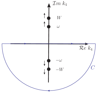
Figure 2: The poles of the modified photon propagator in the complex $k_{4}$ plane and the chosen contour $C$ of integration. The movement of the poles with increasing energy is indicated by small arrows.

With the propagator (11) we get

$$\mathcal{A}_{\text{loop}}=-\sum_{\lambda^{\prime}}e^{4}\frac{1}{(p^{2}-m^{2})^{2}}\varepsilon^{*}_{\sigma}(p_{2},\lambda)\bar{u}(p_{1},s)\gamma^{\sigma}(\hbox{{$p$}\hbox to0.0pt{\hss$/$}}+m)\gamma^{\mu}\\ \times\int\frac{d^{4}q}{(2\pi)^{4}}\frac{(\hbox{{$p$}\hbox to0.0pt{\hss$/$}}-\hbox{{$q$}\hbox to0.0pt{\hss$/$}}+m)}{(p-q)^{2}-m^{2}}\frac{\varepsilon_{\mu}(q,\lambda^{\prime})\varepsilon^{*}_{\mu^{\prime}}(q,\lambda^{\prime})}{q^{2}+2g\lambda^{\prime}(q\cdot n)^{2}\sqrt{D}}\\ \times\gamma^{\mu^{\prime}}(\hbox{{$p$}\hbox to0.0pt{\hss$/$}}+m)\gamma^{\nu}u(p_{1},s)\varepsilon_{\nu}(p_{2},\lambda)\;,$$ (14)

where we have replaced $P^{(\lambda)}_{\mu\nu}$ by employing Eq. (8) in the propagator. The polarization sum over $\lambda^{\prime}$ now runs over all (real and virtual) polarizations of the photon in the loop. By renaming momenta, $k=q$, $k^{\prime}=p-q$ and, using the identity $\int\frac{d^{4}q}{(2\pi)^{4}}=\int\frac{d^{4}k^{\prime}}{(2\pi)^{4}}\int\frac{d^{4}k}{(2\pi)^{4}}\delta^{(4)}(k+k^{\prime}-p)(2\pi)^{4}$ we get

$$\mathcal{A}_{\text{loop}}=-\sum_{\lambda^{\prime}}e^{4}\frac{1}{(p^{2}-m^{2})^{2}}\varepsilon^{*}_{\sigma}(p_{2},\lambda)\bar{u}(p_{1},s)\gamma^{\sigma}(\hbox{{$p$}\hbox to0.0pt{\hss$/$}}+m)\gamma^{\mu}\\ \times\int\frac{d^{4}k^{\prime}}{(2\pi)^{4}}\frac{(\hbox{{$k$}\hbox to0.0pt{\hss$/$}}^{\prime}+m)}{k^{\prime 2}-m^{2}}\int\frac{d^{4}k}{(2\pi)^{4}}\delta^{(4)}(k+k^{\prime}-p_{1}-p_{2})(2\pi)^{4}\\ \times\frac{\varepsilon_{\mu}(k,\lambda^{\prime})\varepsilon^{*}_{\mu^{\prime}}(k,\lambda^{\prime})}{k^{2}+2g\lambda^{\prime}(k\cdot n)^{2}\sqrt{D}}\gamma^{\mu^{\prime}}(\hbox{{$p$}\hbox to0.0pt{\hss$/$}}+m)\gamma^{\nu}u(p_{1},s)\varepsilon_{\nu}(p_{2},\lambda)\;.$$ (15)

We now compute the imaginary part of $\mathcal{A}_{\text{loop}}$ by the computation of the discontinuities of the loop propagators. The integration over $k_{0}$ can be performed by analytic continuation. We go to Euclidean space with the replacement of the zero component of the four-vectors, for a generic four-vector $v$ , $v_{0}=-iv_{4}$ giving the scalar product $vv^{\prime}=-v_{1}v^{\prime}_{1}-v_{2}v^{\prime}_{2}-v_{3}v^{\prime}_{3}-v_{4}v^{\prime}_{4}\equiv-v_{\text{E}}v^{\prime}_{\text{E}}$. The propagator of the photon gives poles for a vanishing denominator, which, in the Euclidean reads

$$k_{E}^{2}(-1+2ig\lambda^{\prime}\left|k_{E}\right|\left|n_{E}\right|^{3}\left|\sin\theta\right|\cos^{2}\theta)=\\ (k_{4}-\omega)(k_{4}+\omega)(-1+2ig\lambda^{\prime}\left|k_{E}\right|\left|n_{E}\right|^{3}\left|\sin\theta\right|\cos^{2}\theta)\;.$$ (16)

Hence, we encounter poles at $\pm\omega$ with

$$\omega=i|\vec{k}|\;,$$ (17)

and two massive ghost modes at $\pm W$ with

$$W=i\sqrt{|\vec{k}|^{2}+M^{2}}\;,\quad M^{2}=\frac{1}{4g^{2}n_{E}^{6}\sin^{2}\theta\cos^{4}\theta}\;.$$ (18)

These poles in the complex $k_{4}$ plane are shown in Fig. 2. With increasing energy $k_{0}$ the poles move along the imaginary axis, departing from the origin, as indicated in the figure. In particular, they never cross the real $k_{4}$ axis. We now close the integration contour along the real $k_{4}$ axis below and pick up the residues in the lower semicircle. The residue at the massive mode at $k_{4}=-W$ will not occur in the phase-space integration and therefore this residue does not contribute to the imaginary part. Therefore we get for the imaginary part of the $k_{4}$ contour integration,

$$i\oint\limits_{C}\frac{\varepsilon_{\mu}(k,\lambda^{\prime})\varepsilon^{*}_{\mu^{\prime}}(k,\lambda^{\prime})dk_{4}}{(k_{4}-\omega)(k_{4}+\omega)(-1+2ig\lambda^{\prime}\left|k_{E}\right|\left|n_{E}\right|^{3}\left|\sin\theta\right|\cos^{2}\theta)}\;,$$ (19)

only a contribution given by the residue at $k_{4}=-\omega=-i|\vec{k}|$, giving

$$i\cdot 2\pi i\lim_{k_{4}\rightarrow-\omega}\frac{\varepsilon_{\mu}(k,\lambda^{\prime})\varepsilon^{*}_{\mu^{\prime}}(k,\lambda^{\prime})}{2\omega}\;.$$ (20)

We see that we only get a contribution to the discontinuity for on-shell photons. Hence, the integration over $k_{0}$ in Eq. (15) singles out the transverse polarization vectors of $\lambda^{\prime}$ and gives a factor $i\pi/k_{0}$.

The integration over $k^{\prime}_{0}$ can be performed as usual, where we close the contour below in the Euclidean,

$$(-i)\oint\limits_{C}\frac{(\hbox{{$k$}\hbox to0.0pt{\hss$/$}}^{\prime}+m)dk^{\prime}_{4}}{(k^{\prime}_{4}-i\sqrt{\vec{k}^{\prime 2}+m^{2}})(k^{\prime}_{4}+i\sqrt{\vec{k}^{\prime 2}+m^{2}})}=\\ (-i)2\pi i\frac{(\hbox{{$k$}\hbox to0.0pt{\hss$/$}}^{\prime}+m)}{2ik_{0}^{\prime}}\;.$$ (21)

Finally, with the spin-sum identity for on-shell fermions $\hbox{{$k$}\hbox to0.0pt{\hss$/$}}^{\prime}+m=\sum_{s^{\prime}}u(k^{\prime},s^{\prime})\bar{u}(k^{\prime},s^{\prime})$ we eventually arrive at the expression for the right-hand-side of Fig. 1, that is Eq. (12). Once again, we stress, that the massive modes of the modified photon propagator do not contribute and unitarity is preserved for the one-loop forward Compton scattering diagram.

Now, the step to one-loop unitarity of the Lorentz-violating model, given by Eq. (1), follows directly: the only contributions to the imaginary part of any one-loop diagram originate from the discontinuities of the propagators, that is, from the poles of the propagators in the loops. In the case of a fermion propagator in the loop, the poles give no additional imaginary contribution with respect to ordinary QED, since the fermion part is unchanged. In the case when a photon propagator appears in the loop, and hence, may get on-shell in the loop integral, the integration over the time-like component can always be written in the form (19). As we have shown, the massive modes of the propagator give no contribution to the imaginary part in the contour integral. Therefore, we conclude that unitarity is preserved at the one-loop order in the model given by the Lorentz-violating Lagrangian (1).

IV Conclusions

Quantum gravity effects may be detected by the investigation of Lorentz-violating terms in the Lagrangian, which are Planck-mass suppressed. One higher-dimensional effective model is the Myers-Pospelev model with a modified kinetic term of the photons. In principle these modification could violate unitarity. Here we have studied unitarity of this model at the one-loop order. Firstly we recalled, how the photon sector has to be modified, giving different photon polarization vectors and a different propagator. We then studied unitarity in forward Compton-scattering at one loop and have shown that unitarity is indeed preserved in this diagram. In particular, we have shown that the additional massive modes of the photon propagator do not contribute to the imaginary part of the loop diagram. Finally, we have generalized this result to an arbitrary one-loop Feynman diagram, that is, the massive modes of the photon give no additional imaginary contributions. This means that unitarity is preserved at the one-loop order.

References

- (1) G. Amelino-Camelia, J. Ellis, N. E. Mavromatos, D. V. Nanopoulos and S. Sarkar, Nature (London) 393, 763 (1998).
- (2) G. Amelino-Camelia, Int. J. Mod. Phys. D 11, 35 (2002); J. Magueijo and L. Smolin, Phys. Rev. Lett. 88, 190403 (2002).
- (3) R. Gambini and J. Pullin, Phys. Rev. D 59, 124021 (1999); J. Alfaro, H. A. Morales-Tecotl and L. F. Urrutia, Phys. Rev. Lett. 84, 2318 (2000).
- (4) V. A. Kostelecky and S. Samuel, Phys. Rev. D 39, 683 (1989); V. A. Kostelecky and S. Samuel, Phys. Rev. D 40, 1886 (1989).
- (5) V. A. Kostelecky and R. Potting, Nucl. Phys. B 359, 545 (1991); V. A. Kostelecky and R. Potting, Phys. Rev. D 51, 3923 (1995).
- (6) D. Colladay and V. A. Kostelecky, Phys. Rev. D 55, 6760 (1997); D. Colladay and V. A. Kostelecky, Phys. Rev. D 58, 116002 (1998).
- (7) V. A. Kostelecky, Phys. Rev. D 69, 105009 (2004); R. Bluhm and V. A. Kostelecky, Phys. Rev. D 71, 065008 (2005).
- (8) R. C. Myers and M. Pospelov, Phys. Rev. Lett. 90, 211601 (2003).
- (9) P. A. Bolokhov and M. Pospelov, Phys. Rev. D 77, 025022 (2008).
- (10) V. A. Kostelecky and M. Mewes, Phys. Rev. D 80, 015020 (2009); V. A. Kostelecky and M. Mewes, Phys. Rev. D 85, 096005 (2012).
- (11) B. Grinstein, D. O’Connell and M. B. Wise, Phys. Rev. D 77, 025012 (2008); J. R. Espinosa, B. Grinstein, D. O’Connell and M. B. Wise, Phys. Rev. D 77, 085002 (2008); J. R. Espinosa and B. Grinstein, Phys. Rev. D 83, 075019 (2011).
- (12) M. Visser, Phys. Rev. D 80, 025011 (2009).
- (13) R. Casana, M. M. Ferreira, Jr., R. V. Maluf and F. E. P. dos Santos, Phys. Lett. B 726, 815 (2013); R. Casana, M. M. Ferreira, Jr, E. Passos and F. E. P. dos Santos, E. O. Silva, Phys. Rev. D 87, 047701 (2013); R. Casana, M. M. Ferreira, R. V. Maluf and F. E. P. dos Santos, Phys. Rev. D 86, 125033 (2012).
- (14) C. M. Reyes, L. F. Urrutia and J. D. Vergara, Phys. Rev. D 78, 125011 (2008); C. M. Reyes, L. F. Urrutia and J. D. Vergara, Phys. Lett. B 675, 336 (2009).
- (15) T. Mariz, Phys. Rev. D 83, 045018 (2011); T. Mariz, J. R. Nascimento and A. Y. .Petrov, Phys. Rev. D 85, 125003 (2012); J. Leite, T. Mariz and W. Serafim, J. Phys. G 40, 075003 (2013).
- (16) L. Maccione, S. Liberati, A. Celotti and J. G. Kirk, J. Cosmol. Astropart. Phys. 10 (2007) 013; L. Maccione and S. Liberati, J. Cosmol. Astropart. Phys. 08 (2008) 027.
- (17) A. Pais and G. E. Uhlenbeck, Phys. Rev. 79, 145 (1950).
- (18) T. D. Lee and G. C. Wick, Nucl. Phys. B9, 209 (1969); T. D. Lee, G. C. Wick, Phys. Rev. D 2, 1033 (1970).
- (19) F. R. Klinkhamer and M. Schreck, Nucl. Phys. B848, 90 (2011); M. Schreck, Phys. Rev. D 86, 065038 (2012); M. Schreck, arXiv:1312.4916 Phys. Rev. D (to be published).
- (20) C. M. Reyes, Phys. Rev. D 87, 125028 (2013); C. M. Reyes, in Proceedings of the Sixth Meeting on CPT and Lorentz Symmetry, Bloomington, IN, USA, 2013 (to be published) arXiv:1307.5341.
- (21) A. A. Andrianov, P. Giacconi and R. Soldati, J. High Energy Phys. 02 (2002) 030; J. Alfaro, A. A. Andrianov, M. Cambiaso, P. Giacconi and R. Soldati, Phys. Lett. B 639, 586 (2006).
- (22) R. E. Cutkosky, J. Math. Phys. 1, 429 (1960); R. E. Cutkosky, P. V. Landshoff, D. I. Olive and J. C. Polkinghorne, Nucl. Phys. B12, 281 (1969).