UV Cascade in Classical Yang-Mills via Kinetic Theory

Abstract

We show that classical Yang-Mills theory with statistically homogeneous and isotropic initial conditions has a kinetic description and approaches a scaling solution at late times. We find the scaling solution by explicitly solving the Boltzmann equations, including all dominant processes (elastic and number-changing). Above a scale $\tilde{p}_{\rm max}\propto t^{\frac{1}{7}}$ the occupancy falls exponentially in $p$. For asymptotically late times and sufficiently small momenta the occupancy scales as $f(p)\propto 1/p$, but this behavior sets in only at very late time scales. We find quantitative agreement of our results with lattice simulations, for times and momenta within the range of validity of kinetic theory.

1 Introduction

Recently there have been a number of studies of classical Yang-Mills theory, motivated by the expectation that it describes quantum Yang-Mills theory in the dual limits of weak coupling and high occupancy. The study of this limit is motivated by arguments that the conditions early after a heavy ion collision are described by the “glasma,” which is precisely such a weak-coupled but high-occupancy state Gelis ; Lappi ; Weigert . Recent theoretical attempts to describe the dynamics of classical Yang-Mills theory KM1 ; BGLMV already differ in some details when describing the simplest case of statistically homogeneous and isotropic, non-expanding initial conditions, which has motivated numerical lattice studies of this limit Berges ; KM3 ; Schlichting .

These studies show that, as expected, classical Yang-Mills theory has no equilibrium state, but features a self-similar cascade of energy from the infrared towards the ultraviolet, with the typical momentum of an excitation rising with time as $t^{\frac{1}{7}}$ and the typical occupancy decaying as $t^{\frac{-4}{7}}$ Berges ; KM3 ; Schlichting . These lattice studies suffer from a limited dynamic and temporal range, statistical errors particularly in the infrared, and lattice spacing corrections. On the other hand, at late times the dynamics should also be well described by kinetic theory. A kinetic study also allows the possibility to better investigate the details of the cascade. For instance, in the kinetic description we can better determine the relative importance of elastic versus inelastic processes, and whether the latter are efficient at all energies or only in the infrared.

Therefore in the current paper we will revisit the problem of the cascade to the ultraviolet in classical Yang-Mills theory, using kinetic theory. In the next section we review the problem, the scales involved, and the form of kinetic theory (with some details about kinetic theory postponed to an appendix).

In Section 4 we introduce two approaches to treating kinetic theory numerically. In Section 5, we find that within the domain of its applicability the kinetic theory reproduces the lattice simulations with great accuracy (see Figure 1), but the treatment is numerically far less demanding. The increased accuracy then allows us to study the scaling solution in far greater detail than on the lattice. In particular, we present evidence that the scaling solution scales as $f(p)\propto 1/p$ (Figure 3). Finally we conclude with a Summary.

2 Boltzmann equation and scaling solution in classical Yang-Mills

Consider quantum Yang-Mills theory where the (t’Hooft) coupling is weak $g^{2}N_{\rm c}\ll 1$, while the mean occupancy is high, $f\gg 1$. In this regime the theory is well described by the classical approximation. If in addition $g^{2}N_{\rm c}f\ll 1$ then the classical theory is in a weakly coupled regime and kinetic theory should be applicable (see e.g. Mueller:2002gd ). Since $g^{2}N_{c}f$ controls the weak-coupling expansion, we will introduce $\bar{f}=g^{2}N_{\rm c}f$; weak coupling is $\bar{f}\ll 1$.

Classical Yang-Mills theory has no equilibrium; if we start off initially with a system where the energy density resides below some scale $p_{\rm max}$, this scale will grow with time. In fact, at late times we expect the occupancy to evolve towards a scaling solution KM3 . To see this, we first introduce a characteristic energy scale $Q$, determined by the energy density $\mathcal{E}$ via

$$Q^{4}=\frac{\pi^{2}g^{2}N_{\rm c}\mathcal{E}}{N_{\rm c}^{2}-1},\qquad\mbox{so}\qquad Q^{4}=\int p^{3}\bar{f}(p)\>dp\quad\mbox{in kinetic theory.}$$ (1)

Next we examine how $\bar{f}(p)$ evolves with time under the Boltzmann equation. For the moment we consider ${2\leftrightarrow 2}$ scatterings;

$$\frac{\partial f(p,t)}{\partial t} = -{\mathcal{C}}_{{2\leftrightarrow 2}}[f(p,t)]\,,$$ (2)

$${\mathcal{C}}_{{2\leftrightarrow 2}}[f_{p}] = \frac{1}{2\nu_{g}}\int\frac{d^{3}k}{(2\pi^{3})}\frac{d^{3}p^{\prime}}{(2\pi^{3})}\frac{d^{3}k^{\prime}}{(2\pi^{3})}\frac{\left|{\overline{{\cal M}}_{pk;p^{\prime}k^{\prime}}^{2}}\right|}{2p2k2p^{\prime}2k^{\prime}}\;(2\pi)^{4}\delta^{4}(p{+}k{-}p^{\prime}{-}k^{\prime})\times$$

$$\hskip 39.83368pt\Big{(}f_{p}f_{k}[1+f_{p^{\prime}}][1+f_{k^{\prime}}]-[1+f_{p}][1+f_{k}]f_{p^{\prime}}f_{k^{\prime}}\Big{)}\,.$$

Here $k$ is the other incoming, and $p^{\prime},k^{\prime}$ the outgoing, momenta, $\left|{\overline{{\cal M}}_{pk;p^{\prime}k^{\prime}}^{2}}\right|$ is the squared matrix element summed (not averaged) over all external colors and spins, and the last line is the difference of the statistical factors for the processes with $p$ as an initial state (first term) and the inverse process with $p$ as a final state (second term). The number of degrees of freedom is denoted by $\nu_{g}$, which for gauge bosons reads $2d_{A}=2(N_{c}^{2}-1)$. Since we consider $f\gg 1$, we may simplify the occupancies,

$$\Big{(}f_{p}f_{k}[1+f_{p^{\prime}}][1+f_{k^{\prime}}]-[1+f_{p}][1+f_{k}]f_{p^{\prime}}f_{k^{\prime}}\Big{)} \simeq f_{p}f_{k}f_{k^{\prime}}+f_{p}f_{k}f_{p^{\prime}}-f_{k}f_{p^{\prime}}f_{k^{\prime}}-f_{p}f_{p^{\prime}}f_{k^{\prime}}\quad$$ (3)

$$= f_{p}f_{k}f_{p^{\prime}}f_{k^{\prime}}\Big{(}f_{p^{\prime}}^{-1}+f_{k^{\prime}}^{-1}-f_{p}^{-1}-f_{k}^{-1}\Big{)}.$$

This simplification amounts to making the classical field approximation.

The external state summed, squared matrix element $\left|{\overline{\cal M}}\right|^{2}$ naturally scales as $g^{4}N_{\rm c}^{2}\nu_{g}$,

$$|\overline{\mathcal{M}}^{2}_{pk;p^{\prime}k^{\prime}}|=2g^{4}N_{\rm c}^{2}\nu_{g}\Big{(}9+\frac{(t-u)^{2}}{s^{2}}+\frac{(s-u)^{2}}{t^{2}}+\frac{(s-t)^{2}}{u^{2}}\Big{)}.$$ (4)

Defining $\left|{\overline{M}^{2}_{pk;p^{\prime}k^{\prime}}}\right|=\left|{\overline{\cal M}}\right|^{2}/(g^{4}N_{\rm c}^{2}\nu_{g})$, we find that factors of $g^{2}N_{\rm c}$ cancel on both sides when we rewrite Eq. (2) in terms of $\bar{f}$ and $\left|{\overline{M}}\right|^{2}$;

$$\frac{d\bar{f}(p,t)}{dt} = -\frac{1}{2}\int\frac{d^{3}k}{(2\pi^{3})}\frac{d^{3}p^{\prime}}{(2\pi^{3})}\frac{d^{3}k^{\prime}}{(2\pi^{3})}\frac{\left|{\overline{M}_{pk;p^{\prime}k^{\prime}}^{2}}\right|}{2p2k2p^{\prime}2k^{\prime}}\;(2\pi)^{4}\delta^{4}(p{+}k{-}p^{\prime}{-}k^{\prime})\times$$ (5)

$$\hskip 39.83368pt\bar{f}_{p}\bar{f}_{k}\bar{f}_{p^{\prime}}\bar{f}_{k^{\prime}}\Big{(}\bar{f}_{p^{\prime}}^{-1}+\bar{f}_{k^{\prime}}^{-1}-\bar{f}_{p}^{-1}-\bar{f}_{k}^{-1}\Big{)}\,.$$

Now assume that the characteristic momentum scale grows as a fractional power of time, $p\propto t^{\alpha}$. By Eq. (1) and energy conservation, the typical occupancy will then fall, $\bar{f}\propto t^{-4\alpha}$. So we introduce dimensionless momentum and occupancy variables which account for this scaling behavior;

$${\tilde{p}}(p,t) \equiv (p/Q)(Qt)^{-\alpha}\qquad\mbox{so}\quad p={\tilde{p}}\,Q(Qt)^{\alpha}\,,$$ (6)

$$\tilde{f}({\tilde{p}},t) \equiv (Qt)^{4\alpha}\bar{f}(p,t)\qquad\mbox{so}\quad\bar{f}(p,t)=\tilde{f}({\tilde{p}},t)(Qt)^{-4\alpha}\,.$$ (7)

In terms of these variables, the lefthand side of the Boltzmann equation becomes

$$\frac{d\bar{f}(p,t)}{dt}=\frac{d[(Qt)^{-4\alpha}\tilde{f}((Qt)^{\alpha}Q{\tilde{p}},t)]}{dt}=(Qt)^{-4\alpha}\;\frac{\alpha}{t}\left(-4\tilde{f}({\tilde{p}})-{\tilde{p}}\frac{\partial\tilde{f}({\tilde{p}},t)}{\partial{\tilde{p}}}+\frac{t}{\alpha}\frac{\partial\tilde{f}({\tilde{p}},t)}{\partial t}\right)\,,$$ (8)

where the last term is the explicit $t$ dependence of $\tilde{f}$, that is, the time dependence not incorporated into the time scaling we have applied. The righthand, collision side of Eq. (5) involves 1 power of momentum since $\left|{\overline{M}}\right|^{2}$ is dimensionless, and it contains three powers of $\bar{f}$; so rescaling in terms of ${\tilde{p}}$ and $\tilde{f}$ scales out a factor of $Q(Qt)^{\alpha}(Qt)^{-12\alpha}=(Qt)^{1-11\alpha}/t$. In order for the left and right hand sides to scale in the same way with $(Qt)$, we must therefore have

$$(Qt)^{-4\alpha}t^{-1}=(Qt)^{1-11\alpha}t^{-1}\qquad\mbox{or}\qquad\alpha=1/7\,.$$ (9)

This reproduces the time scaling behavior found in KM1 ; BGLMV .

Therefore, the Boltzmann equation becomes

$$\frac{t\partial\tilde{f}({\tilde{p}},t)}{\partial t}=\frac{1}{7}\left(4\tilde{f}({\tilde{p}})+{\tilde{p}}\frac{d\tilde{f}({\tilde{p}})}{d{\tilde{p}}}\right)-\tilde{\mathcal{C}}_{{2\leftrightarrow 2}}[\tilde{f}({\tilde{p}})]\,.$$ (10)

Here $\tilde{\mathcal{C}}_{2\leftrightarrow 2}$ is the righthand side of Eq. (5) but with $p,\bar{f}\rightarrow{\tilde{p}},\tilde{f}$. This expression is a relaxation equation for $\tilde{f}$ to approach a “scaling” form where it possesses no explicit time dependence, so the two terms on the righthand side of Eq. (10) cancel. We expect $\tilde{f}$ to approach this scaling form (tracking solution) rather quickly – an expectation supported by lattice studies KM3 – so we will focus on determining the scaling solution itself.

Higher-order scattering processes, that is, those with more participating external lines, are naively suppressed. For instance, a ${2\leftrightarrow 3}$ process would involve an extra vertex, an extra momentum integration, and an extra external state statistical factor. The vertex and statistical factor give rise to a factor of $g^{2}N_{\rm c}f=\bar{f}$. The two powers of momentum in the integration measure $d^{3}l/l$ are canceled by the matrix element becoming dimensionful, $\left|{M}\right|^{2}\sim 1/p^{2}$. So at generic energies and angles, the ${2\leftrightarrow 3}$ process is suppressed, relative to the ${2\leftrightarrow 2}$ process, by a factor of $\bar{f}\sim(Qt)^{-4/7}$. This is why we previously stated that $\bar{f}\ll 1$ is the criterion for perturbative, kinetic behavior.

There are exceptions to this argument, when the matrix element possesses sufficiently strong soft and/or collinear divergences. When such divergences occur, it is necessary to include screening effects to produce finite and correct expressions for the scattering term. In nonabelian gauge theory this is actually already necessary for the ${2\leftrightarrow 2}$ process we have been discussing; $\left|{\overline{M}}\right|^{2}$ is quadratically divergent in the $({\tilde{p}}-{\tilde{p}}^{\prime})\rightarrow 0$ limit, giving rise to a log divergence in Eq. (10) (only logarithmic because $\tilde{f}_{p}^{-1}-\tilde{f}_{p^{\prime}}^{-1}$ nearly cancels in this limit). To handle this divergence correctly, we must incorporate screening effects (Hard Loops) in the computation of $\left|{\overline{M}}\right|^{2}$. The technical complications have been considered elsewhere AMY5 ; we will discuss them a little more in Section 4. Here we just remark that the would-be log divergence is regulated by the scale $m_{{}_{\rm D}}$, which is parametrically

$$m_{{}_{\rm D}}^{2}=4\int\frac{d^{3}p}{(2\pi)^{3}}\frac{\bar{f}(p)}{p}\sim Q^{2}(Qt)^{-2/7}\quad\mbox{so}\quad\frac{m_{{}_{\rm D}}}{p_{\rm max}}\sim\frac{Q(Qt)^{-1/7}}{Q(Qt)^{+1/7}}\sim(Qt)^{-2/7}\,.$$ (11)

Therefore the scale which regulates infrared effects in the collision term actually changes gradually with time. To keep track of this change, we introduce

$$\tilde{m}_{{}_{\rm{D}}}\equiv\frac{m_{{}_{\rm D}}}{Q(Qt)^{1/7}}\quad(\sim(Qt)^{-2/7})$$ (12)

which keeps track of $m_{{}_{\rm D}}$ in the same dimensionless units as we use for momenta ${\tilde{p}}$. Because $\tilde{m}_{{}_{\rm{D}}}$ varies with time, our argument for a scaling solution is not quite correct. Because the time dependence of $\tilde{m}_{{}_{\rm{D}}}$ is very weak we expect this to be a minor effect and we will still seek a scaling solution.

The Debye scale also plays the role of the infrared scale beyond which the kinetic theory description is no longer reliable. This is because our kinetic description assumes that the dispersion relation is lightlike and the spectral function carries all its weight on a quasiparticle pole, properties which break down at this scale. Therefore our results are not to be trusted at and below the scale ${\tilde{p}}=\tilde{m}_{{}_{\rm{D}}}$.

We saw above that, at generic momenta and angles, higher-leg processes are suppressed. But they are unsuppressed in any soft or collinear phase space region where they are sufficiently soft and collinear divergent. We see from the above arguments that to be relevant at late times, a ${2\leftrightarrow 3}$ process must be quadratically soft and/or collinear divergent to introduce a factor of ${\tilde{p}}^{2}/\tilde{m}_{{}_{\rm{D}}}^{2}\sim(Qt)^{4/7}$ which compensates the factor $\bar{f}\sim(Qt)^{-4/7}$. Additional lines require stronger power divergences. Arnold, Moore, and Yaffe showed that sufficiently strong divergences occur only in $n\leftrightarrow(n+1)$ processes; and that such processes can be treated in terms of an effective ${1\leftrightarrow 2}$ process AMY5 . We show in Appendix A that in the current context these ${1\leftrightarrow 2}$ processes scale with time in the same way as ${2\leftrightarrow 2}$ processes and must be included in the collision term. Explicitly, Eq. (10) becomes

$$0=\frac{1}{7}\left(4\tilde{f}({\tilde{p}})+{\tilde{p}}\frac{d\tilde{f}({\tilde{p}})}{d{\tilde{p}}}\right)-\tilde{\mathcal{C}}_{2\leftrightarrow 2}[\tilde{f}({\tilde{p}})]-\tilde{\mathcal{C}}_{1\leftrightarrow 2}[\tilde{f}({\tilde{p}})]\,,$$ (13)

where

$$\tilde{\mathcal{C}}_{2\leftrightarrow 2}[\tilde{f}({\tilde{p}})] = \frac{1}{2}\int\frac{d^{3}{\tilde{k}}}{(2\pi^{3})}\frac{d^{3}{\tilde{p}}^{\prime}}{(2\pi^{3})}\frac{d^{3}{\tilde{k}}^{\prime}}{(2\pi^{3})}\frac{\left|{\overline{M}_{{\tilde{p}}{\tilde{k}};{\tilde{p}}^{\prime}{\tilde{k}}^{\prime}}^{2}}\right|}{2{\tilde{p}}2{\tilde{k}}2{\tilde{p}}^{\prime}2{\tilde{k}}^{\prime}}\;(2\pi)^{4}\delta^{4}({\tilde{p}}{+}{\tilde{k}}{-}{\tilde{p}}^{\prime}{-}{\tilde{k}}^{\prime})\times$$ (14)

$$\hskip 39.83368pt\tilde{f}_{{\tilde{p}}}\tilde{f}_{{\tilde{k}}}\tilde{f}_{{\tilde{p}}^{\prime}}\tilde{f}_{{\tilde{k}}^{\prime}}\Big{(}\tilde{f}_{{\tilde{p}}^{\prime}}^{-1}+\tilde{f}_{{\tilde{k}}^{\prime}}^{-1}-\tilde{f}_{{\tilde{p}}}^{-1}-\tilde{f}_{{\tilde{k}}}^{-1}\Big{)}$$

and

$$\tilde{\mathcal{C}}_{1\leftrightarrow 2}[\tilde{f}({\tilde{p}})] = \frac{(2\pi)^{3}}{{\tilde{p}}^{2}}\int_{0}^{\frac{{\tilde{p}}}{2}}d{\tilde{k}}\>\tilde{\gamma}^{g}_{gg}({\tilde{p}};{\tilde{k}},{\tilde{p}}{-}{\tilde{k}})\Big{(}\tilde{f}_{\tilde{p}}\tilde{f}_{{\tilde{p}}{-}{\tilde{k}}}+\tilde{f}_{\tilde{p}}\tilde{f}_{\tilde{k}}-\tilde{f}_{\tilde{k}}\tilde{f}_{{\tilde{p}}{-}{\tilde{k}}}\Big{)}$$ (15)

$$+\frac{(2\pi)^{3}}{{\tilde{p}}^{2}}\int_{0}^{\infty}d{\tilde{k}}\>\tilde{\gamma}^{g}_{gg}({\tilde{p}}{+}{\tilde{k}};{\tilde{p}},{\tilde{k}})\Big{(}\tilde{f}_{\tilde{p}}\tilde{f}_{\tilde{k}}-\tilde{f}_{\tilde{p}}\tilde{f}_{{\tilde{p}}{+}{\tilde{k}}}-\tilde{f}_{\tilde{k}}\tilde{f}_{{\tilde{p}}{+}{\tilde{k}}}\Big{)}\,;$$

this term is explained and the splitting rate $\tilde{\gamma}^{g}_{gg}$ is defined in Appendix A.

3 IR and UV limiting behaviors

Before solving Eq. (13), it is useful to study analytically how the solution should scale with ${\tilde{p}}$ in the IR and in the UV. Knowing the scaling behavior will also be helpful when we attempt a numerical solution.

We begin with the UV limiting behavior. We expect the large ${\tilde{p}}$ behavior of $\tilde{f}({\tilde{p}})$ to be exponential, $\tilde{f}({\tilde{p}})\rightarrow{\tilde{p}}^{a}\exp(-b{\tilde{p}})$ for some $a,b$. To see this, note first that, for the energy to be bounded, the occupancy in the tail has to fall faster than $\tilde{f}\propto{\tilde{p}}^{-4}$. But in any region where $|{\tilde{p}}d\tilde{f}/d{\tilde{p}}|>4\tilde{f}$, Eq. (8) shows that $d\bar{f}/dt>0$ – scatterings must move particles into the UV tail, at a rate comparable to the system age. Exponential behavior is self-consistent, because to produce a particle with ${\tilde{p}}\gg 1$ one must scatter or merge together particles of energies totalling at least ${\tilde{p}}$; exponential behavior means that the final state occupancy scales with the likelihood of finding two constituents which are available to merge. Stimulation factors do not change this argument. Super-exponential behavior such as $\tilde{f}\sim\exp(-k{\tilde{p}}^{2})$ can be excluded, because there are far more pairs of particles of energy ${\tilde{p}}/2$ available than particles of energy ${\tilde{p}}$; so the merger rate to momentum scale ${\tilde{p}}$ would greatly exceed the occupancy there. Similarly, power-law UV behavior cannot provide enough scatterings to keep the tail growing.

To explore the infrared behavior of $\tilde{f}({\tilde{p}})$, it is useful to consider total particle number. By integrating the Boltzmann equation, Eq. (13), over momentum $\int\frac{d^{3}{\tilde{p}}}{(2\pi)^{3}}$, we obtain an equation describing total particle number change;

$$\int\frac{{\tilde{p}}^{2}d{\tilde{p}}}{2\pi^{2}}\left(\left[\frac{4}{7}\tilde{f}_{\tilde{p}}+\frac{{\tilde{p}}d\tilde{f}_{\tilde{p}}}{7d{\tilde{p}}}\right]-\tilde{\mathcal{C}}_{{1\leftrightarrow 2}}[\tilde{f}_{\tilde{p}}]-\tilde{\mathcal{C}}_{{2\leftrightarrow 2}}[\tilde{f}_{\tilde{p}}]\right)=0\,.$$ (16)

The contribution from the term in square brackets is

$$\frac{1}{14\pi^{2}}\int{\tilde{p}}^{2}\Big{(}4\tilde{f}_{\tilde{p}}+{\tilde{p}}\tilde{f}^{\prime}_{\tilde{p}}\Big{)}d{\tilde{p}}=\frac{1}{14\pi^{2}}\int{\tilde{p}}^{2}\tilde{f}_{\tilde{p}}\>d{\tilde{p}}=\frac{\tilde{n}}{7}$$ (17)

which (up to our rescalings by factors of $g^{2}N_{\rm c}$ and $(Qt)$) is just minus the time rate of change of particle number, $-tdn/dt=n/7$, which is finite. The contribution from ${2\leftrightarrow 2}$ processes is, unsurprisingly, zero;

$$\int\frac{d^{3}{\tilde{p}}}{(2\pi)^{3}}\>\tilde{\mathcal{C}}_{{2\leftrightarrow 2}}[\tilde{f}_{\tilde{p}}] = \int\frac{d^{3}{\tilde{p}}\,d^{3}{\tilde{k}}\,d^{3}{\tilde{p}}^{\prime}\,d^{3}{\tilde{k}}^{\prime}}{(2\pi)^{9}}\frac{\left|{\overline{M}^{2}_{{\tilde{p}}{\tilde{k}};{\tilde{p}}^{\prime}{\tilde{k}}^{\prime}}}\right|^{2}}{16{\tilde{p}}{\tilde{k}}{\tilde{p}}^{\prime}{\tilde{k}}^{\prime}}(2\pi)^{4}\delta^{4}({\tilde{p}}{+}{\tilde{k}}{-}{\tilde{p}}^{\prime}{-}{\tilde{k}}^{\prime})$$ (18)

$$\hskip 68.28644pt\times\tilde{f}_{\tilde{p}}\tilde{f}_{\tilde{k}}\tilde{f}_{{\tilde{p}}^{\prime}}\tilde{f}_{{\tilde{k}}^{\prime}}\Big{(}\tilde{f}_{{\tilde{p}}^{\prime}}^{-1}+\tilde{f}_{{\tilde{k}}^{\prime}}^{-1}-\tilde{f}_{{\tilde{p}}}^{-1}-\tilde{f}_{{\tilde{k}}}^{-1}\Big{)}$$

which vanishes since the first line is symmetric, and the second antisymmetric, on exchanging primed and unprimed variables. The contribution from ${1\leftrightarrow 2}$ processes is $\int\frac{d^{3}{\tilde{p}}}{(2\pi)^{3}}$ of Eq. (15), which is

$$\int\frac{d^{3}{\tilde{p}}}{(2\pi)^{3}}\tilde{\mathcal{C}}_{{1\leftrightarrow 2}}[\tilde{f}_{\tilde{p}}] = \phantom{+}4\pi\int_{0}^{\infty}d{\tilde{p}}\int_{0}^{{\tilde{p}}/2}d{\tilde{k}}\>\tilde{\gamma}^{g}_{gg}({\tilde{p}};{\tilde{k}},{\tilde{p}}-{\tilde{k}})\Big{(}\tilde{f}_{\tilde{p}}\tilde{f}_{{\tilde{p}}-{\tilde{k}}}+\tilde{f}_{\tilde{p}}\tilde{f}_{{\tilde{k}}}-\tilde{f}_{{\tilde{k}}}\tilde{f}_{{\tilde{p}}-{\tilde{k}}}\Big{)}$$ (19)

$$+4\pi\int_{0}^{\infty}d{\tilde{p}}d{\tilde{k}}\>\tilde{\gamma}^{g}_{gg}({\tilde{p}}+{\tilde{k}};{\tilde{k}},{\tilde{p}})\Big{(}\tilde{f}_{\tilde{p}}\tilde{f}_{{\tilde{k}}}-\tilde{f}_{{\tilde{p}}+{\tilde{k}}}\tilde{f}_{{\tilde{k}}}-\tilde{f}_{{\tilde{p}}+{\tilde{k}}}\tilde{f}_{{\tilde{p}}}\Big{)}\,.$$

To make the two terms look more similar we rename ${\tilde{p}}$ in the first equation to ${\tilde{p}}{+}{\tilde{k}}$;

$$\int\frac{d^{3}{\tilde{p}}}{(2\pi)^{3}}\tilde{\mathcal{C}}_{{1\leftrightarrow 2}}[\tilde{f}_{\tilde{p}}] = \phantom{+}4\pi\int_{{\tilde{p}}>{\tilde{k}}}d{\tilde{p}}d{\tilde{k}}\;\tilde{\gamma}^{g}_{gg}({\tilde{p}}+{\tilde{k}};{\tilde{k}},{\tilde{p}})\Big{(}\tilde{f}_{{\tilde{p}}+{\tilde{k}}}\tilde{f}_{{\tilde{p}}}+\tilde{f}_{{\tilde{p}}+{\tilde{k}}}\tilde{f}_{{\tilde{k}}}-\tilde{f}_{{\tilde{k}}}\tilde{f}_{{\tilde{p}}}\Big{)}$$ (20)

$$+4\pi\int_{0}^{\infty}d{\tilde{p}}d{\tilde{k}}\;\tilde{\gamma}^{g}_{gg}({\tilde{p}}+{\tilde{k}};{\tilde{k}},{\tilde{p}})\Big{(}\tilde{f}_{\tilde{p}}\tilde{f}_{{\tilde{k}}}-\tilde{f}_{{\tilde{p}}+{\tilde{k}}}\tilde{f}_{{\tilde{k}}}-\tilde{f}_{{\tilde{p}}+{\tilde{k}}}\tilde{f}_{{\tilde{p}}}\Big{)}\,,$$

which makes it clear that the first term is minus half the second term. The rate of particle number destruction is therefore

$$4\pi\int_{{\tilde{p}}>{\tilde{k}}}d{\tilde{p}}d{\tilde{k}}\;\tilde{\gamma}^{g}_{gg}({\tilde{p}}+{\tilde{k}};{\tilde{k}},{\tilde{p}})\>\tilde{f}_{{\tilde{p}}{+}{\tilde{k}}}\tilde{f}_{\tilde{p}}\tilde{f}_{\tilde{k}}\Big{(}\tilde{f}^{-1}_{{\tilde{p}}+{\tilde{k}}}-\tilde{f}^{-1}_{{\tilde{p}}}-\tilde{f}^{-1}_{{\tilde{k}}}\Big{)}=\frac{\tilde{n}}{7}\,,$$ (21)

where we used Eq. (16) and Eq. (17) to equate the integral to the particle number. Note that if $\tilde{f}_{\tilde{p}}$ is steeper than ${\tilde{p}}^{-1}$ at all ${\tilde{p}}$, then the lefthand side is everywhere positive.

Since the particle number is finite, the lefthand side of Eq. (21) must also be finite. The danger is of a divergence at small ${\tilde{k}}$. In this limit $\tilde{\gamma}^{g}_{gg}$ behaves as

$$\lim_{{\tilde{k}}\ll 1,{\tilde{p}}}\tilde{\gamma}^{g}_{gg}({\tilde{p}}+{\tilde{k}};{\tilde{p}},{\tilde{k}})\propto\frac{1}{{\tilde{k}}}\quad\mbox{and independent of ${\tilde{p}}$.}$$ (22)

(This fact is familiar from the physics of initial state radiation, where it gives rise to the log soft divergence in the total emission rate.) The product of statistical functions must therefore remain finite in this limit. If $\tilde{f}_{\tilde{k}}$ grows faster than ${\tilde{k}}^{-1}$ in the infrared, then $\tilde{f}^{-1}_{\tilde{k}}$ falls faster than linearly and can be neglected. Then approximating $\tilde{f}^{-1}_{{\tilde{p}}+{\tilde{k}}}-\tilde{f}^{-1}_{{\tilde{p}}}\simeq{\tilde{k}}\,d\tilde{f}^{-1}_{\tilde{p}}/d{\tilde{p}}>0$, we find that the integral is small ${\tilde{k}}$ divergent. Therefore $\tilde{f}_{\tilde{k}}$ cannot grow faster than ${\tilde{k}}^{-1}$ in the infrared, in order for the particle destruction rate to remain finite, within the kinetic description we have followed.

Note that, since $\tilde{m}_{{}_{\rm{D}}}$ is finite and the quoted behavior for $\tilde{\gamma}$ is only valid for ${\tilde{k}}\geq\tilde{m}_{{}_{\rm{D}}}$, this argument is only rigorous if $\tilde{m}_{{}_{\rm{D}}}\ll 1$, meaning at late times. Nevertheless, what it shows is that, at sufficiently late times and deep enough in the infrared, the behavior of the occupancy must scale as $f\propto p^{-1}$, not a steeper power such as $p^{-4/3}$. This is in contrast to what one might guess based on certain cascade arguments Berges .

4 Solving the Boltzmann equation

We have developed two methods for solving the Boltzmann equation, a variational method which is specialized to the problem at hand and a time-domain, momentum-discretization approach which should have wider applications. We will present each approach in turn.

4.1 Variational formulation

Eq. (13) admits a one parameter family of solutions corresponding to the arbitrary initial value of the energy density. Defining

$$\epsilon[\tilde{f}]=\int d{\tilde{p}}~{}{\tilde{p}}^{3}~{}\tilde{f}_{{\tilde{p}}}$$ (23)

and recalling our definitions, Eq. (1), Eq. (6) and Eq. (7), we are seeking the unique function $\tilde{f}({\tilde{p}})$ which satisfies Eq. (13) with $\epsilon[\tilde{f}]=1$. We will make the problem variational by specifying an action $\Gamma[\tilde{f}]$ which reaches its extremum when Eq. (13) and the condition $\epsilon[\tilde{f}]=1$ are satisfied. Integrating over the sphere,

$$\int{\tilde{p}}^{2}\frac{d\Omega}{(2\pi)^{2}}=\frac{{\tilde{p}}^{2}}{\pi}$$ (24)

we will now define the operators

$$L[\tilde{f}_{{\tilde{p}}}] = \frac{{\tilde{p}}^{2}}{7\pi}\Big{(}4\tilde{f}_{{\tilde{p}}}+{\tilde{p}}\tilde{f}^{\prime}_{{\tilde{p}}}\Big{)}$$ (25)

$$C[\tilde{f}_{{\tilde{p}}}]=C_{{1\leftrightarrow 2}}[\tilde{f}_{{\tilde{p}}}]+C_{{2\leftrightarrow 2}}[\tilde{f}_{{\tilde{p}}}] = \frac{{\tilde{p}}^{2}}{\pi}\Big{(}\tilde{\mathcal{C}}_{{2\leftrightarrow 2}}[\tilde{f}_{{\tilde{p}}}]+\tilde{\mathcal{C}}_{{1\leftrightarrow 2}}[\tilde{f}_{{\tilde{p}}}]\Big{)}$$ (26)

and choose the action to be

$$\Gamma[\tilde{f}]=\lambda\Big{(}\epsilon[\tilde{f}]-1\Big{)}^{2}+\int\frac{d{\tilde{p}}}{2\pi}{\tilde{p}}^{2\alpha}\Big{(}L[\tilde{f}_{{\tilde{p}}}]-C[\tilde{f}_{{\tilde{p}}}]\Big{)}^{2}\,.$$ (27)

For any choice of $\alpha$ and $\lambda>0$ this action is nonnegative definite, but it equals zero where Eq. (13) is satisfied; therefore it is a good starting point for a variational solution.

There remain technical issues, both in the computation of $\gamma^{g}_{gg}$ and in the handling of the multiple integrals involved in $C_{{2\leftrightarrow 2}}$. We postpone these to Appendix A and Appendix B respectively.

Concerning the inclusion of a screening mass, it was mentioned in the previous section that its presence would break the otherwise exact scaling law. To proceed onwards, we will simply fix the value of $\tilde{m}_{{}_{\rm{D}}}$, which is a reasonable approximation since the actual dependence on $\tilde{m}_{{}_{\rm{D}}}$ is weak.

Since $\tilde{f}({\tilde{p}})$ has an infinite number of degrees of freedom, we must make some simplifications in order to seek an extremum. We choose to extremize $\tilde{f}({\tilde{p}})$ over some flexible but finite-parameter Ansatz; specifically we will consider

$$\tilde{f}({\tilde{p}})=A\Big{(}\frac{{\tilde{p}}}{\omega_{1}}\Big{)}^{g_{1}({\tilde{p}})}e^{-\beta{\tilde{p}}^{g_{2}({\tilde{p}})}\frac{{\tilde{p}}^{\gamma}}{{\tilde{p}}^{\gamma}+\omega_{2}^{\gamma}}}$$ (28)

where $g_{1}$ and $g_{2}$ are rational functions of the form

$$g_{i}({\tilde{p}})=\frac{a_{i,N_{i}}({\tilde{p}}/\lambda_{i})^{N_{i}}+...+a_{i,0}}{b_{i,N_{i}}({\tilde{p}}/\lambda_{i})^{N_{i}}+...+1}.$$ (29)

The variational coefficients are $c_{i}\in\{A,\omega_{1},\beta,\gamma,\omega_{2},a_{1,0}...\}$. Physically $\beta$ and $g_{2}$ control the UV behavior, while $g_{1}$ primarily controls the IR behavior. The extremal value within this Ansatz is the choice of $c_{i}$ such that

$$\frac{\partial}{\partial c_{i}}\Gamma[\tilde{f}_{{\tilde{p}}}]=0.$$ (30)

In the limit where the Ansatz is described by an infinite number of parameters, this equation in principle becomes exact. The extremal point of $\Gamma$ can be located iteratively by a numerical implementation of non-linear conjugate gradient descent, and the failure to satisfy Eq. (13) exactly can be assessed by plotting $L[\tilde{f}_{{\tilde{p}}}]$ and $C[\tilde{f}_{{\tilde{p}}}]$ as functions of ${\tilde{p}}$ and seeing with what accuracy they cancel.

4.2 Discrete-momentum method

The second implementation of the Boltzmann equation we have used involves the direct time evolution of a momentum-discretized version of Eq. (10) (naturally including both $\tilde{\mathcal{C}}_{2\leftrightarrow 2}$ and $\tilde{\mathcal{C}}_{1\leftrightarrow 2}$). We do so by introducing a discrete sample of points ${\tilde{p}}_{i}$ and tracking the number density of particles with momentum near ${\tilde{p}}_{i}$, $\tilde{n}_{i}$. Specifically, a continuous distribution $\tilde{f}(p)$ is converted into the discrete $\tilde{n}_{i}$ via

$$\tilde{n}_{i}\equiv\int\frac{d^{3}{\tilde{p}}}{(2\pi)^{3}}\tilde{f}({\tilde{p}})w_{i}({\tilde{p}})\,,\qquad w_{i}({\tilde{p}})\equiv\left\{\begin{array}[]{ll}\frac{{\tilde{p}}-{\tilde{p}}_{i-1}}{{\tilde{p}}_{i}-{\tilde{p}}_{i-1}}\,,&{\tilde{p}}_{i-1}<{\tilde{p}}<{\tilde{p}}_{i}\\ \frac{{\tilde{p}}_{i+1}-{\tilde{p}}}{{\tilde{p}}_{i+1}-{\tilde{p}}_{i}}\,,&{\tilde{p}}_{i}<{\tilde{p}}<{\tilde{p}}_{i+1}\\ 0&{\tilde{p}}<{\tilde{p}}_{i-1}\mbox{ or }{\tilde{p}}>{\tilde{p}}_{i+1}\,.\\ \end{array}\right.$$ (31)

Here the “wedge” function $w_{i}({\tilde{p}})$ rises linearly from $0$ at ${\tilde{p}}_{i-1}$ to 1 at ${\tilde{p}}_{i}$ and then falls to zero linearly at ${\tilde{p}}_{i+1}$, so $\sum_{i}w_{i}({\tilde{p}})=1$ for any ${\tilde{p}}$ within the range considered. The points ${\tilde{p}}_{i}$ need not be evenly spaced and in practice it is best to space them more tightly where $\tilde{f}$ shows stronger variation. In terms of the $\tilde{n}_{i}$, the particle number and energy densities are

$$\tilde{n}=\sum_{i}\tilde{n}_{i}\,,\qquad\epsilon=\sum_{i}{\tilde{p}}_{i}\tilde{n}_{i}\,.$$ (32)

The time evolution of $\tilde{n}_{i}$ is determined by integrating Eq. (10) over ${\tilde{p}}$,

$$t\partial_{t}\tilde{n}_{i}=\frac{1}{7}\left(4\tilde{n}_{i}+{\tilde{p}}\frac{d\tilde{n}}{d{\tilde{p}}}\right)-\int\frac{d^{3}{\tilde{p}}}{(2\pi)^{3}}w_{i}({\tilde{p}})(\tilde{\mathcal{C}}_{1\leftrightarrow 2}({\tilde{p}})+\tilde{\mathcal{C}}_{2\leftrightarrow 2}({\tilde{p}}))\,.$$ (33)

The equation is evolved until it converges, yielding the scaling solution for $\tilde{n}_{i}$.

Using Eq. (14), the collision term is

$$\int\frac{d^{3}{\tilde{p}}}{(2\pi)^{3}}w_{i}({\tilde{p}})\tilde{\mathcal{C}}_{2\leftrightarrow 2} = \frac{1}{8}\int\frac{d^{3}{\tilde{p}}d^{3}{\tilde{k}}d^{3}{\tilde{p}}^{\prime}d^{3}{\tilde{k}}^{\prime}}{(2\pi)^{12}}\frac{\left|{\overline{M}_{{\tilde{p}}{\tilde{k}};{\tilde{p}}^{\prime}{\tilde{k}}^{\prime}}^{2}}\right|}{2{\tilde{p}}2{\tilde{k}}2{\tilde{p}}^{\prime}2{\tilde{k}}^{\prime}}\;(2\pi)^{4}\delta^{4}({\tilde{p}}{+}{\tilde{k}}{-}{\tilde{p}}^{\prime}{-}{\tilde{k}}^{\prime})\times$$

$$\hskip 10.00002pt\tilde{f}_{{\tilde{p}}}\tilde{f}_{{\tilde{k}}}\tilde{f}_{{\tilde{p}}^{\prime}}\tilde{f}_{{\tilde{k}}^{\prime}}\Big{(}\tilde{f}_{{\tilde{p}}^{\prime}}^{-1}{+}\tilde{f}_{{\tilde{k}}^{\prime}}^{-1}{-}\tilde{f}_{{\tilde{p}}}^{-1}{-}\tilde{f}_{{\tilde{k}}}^{-1}\Big{)}\Big{(}w_{i}({\tilde{p}}){+}w_{i}({\tilde{k}}){-}w_{i}({\tilde{p}}^{\prime}){-}w_{i}({\tilde{k}}^{\prime})\Big{)}$$

and similarly for Eq. (15). In the numerical implementation all $\partial_{t}\tilde{n}_{i}$ are computed simultaneously; the values of $p,p^{\prime},k,k^{\prime}$ are sampled, and each sample point then contributes to the eight $\partial_{t}\tilde{n}_{i}$ for which a $w_{i}$ function is nonzero. This approach identically conserves total energy and violates particle number by precisely the amount stipulated in Eq. (21) – in particular the $2\leftrightarrow 2$ process exactly conserves particle number under this implementation.

So far the implementation we have described is an exact representation of the original Boltzmann equation. The implementation becomes approximative because we must deal with two quantities which are not strictly well defined in terms of the $\tilde{n}_{i}$ alone. The first is ${\tilde{p}}\frac{d\tilde{n}}{d{\tilde{p}}}$, appearing in Eq. (33). We can fix it uniquely by the requirement that the rescaling of momentum and occupancy with time, introduced in Eq. (6) and Eq. (7), identically preserves particle number and energy. This leads to

$${\tilde{p}}\frac{d\tilde{n}_{i}}{d{\tilde{p}}}\equiv-\tilde{n}_{i}\frac{{\tilde{p}}_{i}}{{\tilde{p}}_{i}-{\tilde{p}}_{i-1}}+\tilde{n}_{i+1}\frac{{\tilde{p}}_{i+1}}{{\tilde{p}}_{i+1}-{\tilde{p}}_{i}}\,.$$ (35)

The other quantity we must deal with is the occupancy $\tilde{f}_{\tilde{p}}$ appearing in Eq. (4.2). We interpolate this from the $n_{i}$; for $p_{i}<p<p_{i+1}$ we use

$$4\pi p^{2}\tilde{f}(p)=\frac{2\tilde{n}_{i}}{{\tilde{p}}_{i+1}-{\tilde{p}}_{i-1}}\frac{{\tilde{p}}_{i+1}-{\tilde{p}}}{{\tilde{p}}_{i+1}-{\tilde{p}}_{i}}+\frac{2\tilde{n}_{i+1}}{{\tilde{p}}_{i+2}-{\tilde{p}}_{i}}\frac{{\tilde{p}}-{\tilde{p}}_{i}}{{\tilde{p}}_{i+1}-{\tilde{p}}_{i}}\,.$$ (36)

The need for this inerpolation means that the method is not exact. However, discretization errors in this approach should scale as the second power of the ${\tilde{p}}_{i}$ spacing. Numerically it is not difficult to implement 200 or more points. In the discrete momentum method, we can set $\tilde{m}_{{}_{\rm{D}}}$ by hand as in the Ansatz method, or we can determine $\tilde{m}_{{}_{\rm{D}}}$ self-consistently as an integral moment of the distribution as a function of time.

5 Results and discussion

As mentioned before, the cascade to the UV does not quite achieve a scaling solution, because the Debye scale evolves relative to the characteristic momentum: $\tilde{m}_{{}_{\rm{D}}}\sim(Qt)^{-2/7}$. Therefore we must fix a value of $\tilde{m}_{{}_{\rm{D}}}$ and determine the scaling solution at that epoch. Figure 1 shows the scaling solution we find when $\tilde{m}_{{}_{\rm{D}}}=0.08$ (corresponding to time $Qt=2000$). The figure shows the results using kinetic theory solved via the momentum discretization method and via the Ansatz method. The curves are nearly identical, except far in the infrared, ${\tilde{p}}<0.1$, where the Ansatz method loses resolution and where kinetic theory no longer accurately describes the full (hard-loop) dynamics.

The figure also compares the kinetic theory results with the direct determination of the occupancies, established by solving the classical theory on the lattice. The lattice data are also evaluated at time $(Qt)=2000$, when the occupancies self-consistently return a value $\tilde{m}_{{}_{\rm{D}}}\simeq 0.08$. In the infrared it is important to use a large volume and high statistics, so we have averaged our results over 6 independent evolutions with $(Qa)=0.2$ and $(QL)=51.2$. In the ultraviolet it is important to extrapolate carefully to the small lattice-spacing limit, so we have extrapolated over three spacings down to $(Qa)=0.1$, with half the box length (the results remain unchanged if we halve the box size again). These results are shown in Figure 1 as red and blue circles, respectively. Without the continuum extrapolation the UV tail would not fit the kinetic theory result. All lattice data are based on Coulomb gauge-fixed transverse electric field correlators, using dispersion corrected for plasma frequency effects as described in Ref. KM3 .

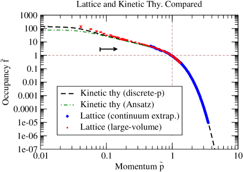
Figure 1: Scaling solution for the occupancy, when $\tilde{m}_{{}_{\rm{D}}}=0.08$. Kinetic theory results use the momentum discretization method (dashed black line) and via the Ansatz method (green dash-dotted curve). Lattice results are shown using a large volume (red circles, used in the IR) and a smaller volume but with careful extrapolation to the continuum limit (blue circles, used in the UV). The beginning of the arrow marks the scale $\tilde{m}_{{}_{\rm{D}}}$ above which the lattice and kinetic theory results should agree.

The figure shows clearly that kinetic theory provides an excellent description of the lattice results for the scaling solution of the UV cascade, except in the infrared, ${\tilde{p}}<0.1$. Note however that the kinetic theory we have used is only strictly valid in the momentum region $p\gg m_{{}_{\rm D}}$, marked by the black arrow in the figure. In particular, when computing the collision operator ${\mathcal{C}}_{{2\leftrightarrow 2}}$ we have treated the external states with massless dispersion and made Hard Thermal Loop approximations in the matrix elements (and the approximations described in Appendix B) which are not reliable in this regime. In addition we have continued to treat the ${\mathcal{C}}_{{1\leftrightarrow 2}}$ splitting process in a collinear expansion which also loses its reliability for $p\mbox{~{}{\raisebox{1.72218pt}{$<$}} {\raisebox{-2.58334pt}{$\sim$}}~{}}m_{{}_{\rm D}}$. We believe that one could in principle improve kinetic theory such that it incorporates these effects in the IR, but to our knowledge this has not been done.

One advantage of having a kinetic description of the full problem is that we can determine what physics is most important in controlling the evolution of the particle cascade. To explore this, we compare the relative sizes of ${\mathcal{C}}_{{2\leftrightarrow 2}}$ and ${\mathcal{C}}_{{1\leftrightarrow 2}}$, as a function of momentum, in Figure 2. The solid (black) line in the figure shows the total occupancy evolution $(t/f)df/dt$, which switches from negative below ${\tilde{p}}=1.1$ (particle number leaving the infrared) to positive above ${\tilde{p}}=1.1$ (particle number filling into the ultraviolet). The results for the ${1\leftrightarrow 2}$ and ${2\leftrightarrow 2}$ collision processes are shown in red dash-dot and blue dashed, respectively. We see that the ${1\leftrightarrow 2}$ processes raise particle number in the UV above ${\tilde{p}}=1.1$ and remove particle number in the IR, while the ${2\leftrightarrow 2}$ processes raise particle number both in the UV (energy cascade) and IR (particle number cascade), while removing particles in the range $0.2<{\tilde{p}}<1.2$.

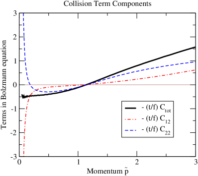
Figure 2: Components of the Boltzmann equation, expressed as relative contributions to the particle number evolution $(t/f)df/dt$, computed with the discrete momentum method with $\tilde{m}_{{}_{\rm{D}}}=0.08$. ${1\leftrightarrow 2}$ processes (red dash-dot), ${2\leftrightarrow 2}$ processes (blue dashes), the sum (black solid).

The Figure 2, along with an analysis of the details of each collision term, give us information about what the most important processes are in each momentum range. The figure shows that the cascade filling the UV modes is a mixture of the two collision processes. Since the ${2\leftrightarrow 2}$ process is enhanced by $\log(1/\tilde{m}_{{}_{\rm{D}}})$, its relative importance gradually increases as the occupancy falls with time. On the other hand, the deep infrared is controlled by a competition between the two processes, with a large rate of particles entering the IR via ${2\leftrightarrow 2}$ processes and a large removal rate via ${1\leftrightarrow 2}$ processes. The IR occupancy is determined by the requirement that these rates be in balance.

What are the typical momenta involved in these IR occupancy establishing processes? We find that the typical ${2\leftrightarrow 2}$ process is one involving a small-exchange-momentum collision between an IR particle and a typical (${\tilde{p}}\sim 1$) particle. The typical ${1\leftrightarrow 2}$ process involves a soft particle being absorbed onto a typical (${\tilde{p}}\sim 1$) particle. In particular, when ${\tilde{p}}\ll 1$, Eq. (15) is dominated by ${\tilde{k}}\sim 1$, not by ${\tilde{k}}\sim{\tilde{p}}$. This is confirmed by the numerics. Therefore the processes which establish the occupancy in the regime ${\tilde{p}}\ll 1$ are not dominated by scatterings between particles of comparable momentum, but involve scatterings between soft particles and typical particles with ${\tilde{p}}\sim 1$. This means that the conditions for an energy cascade Berges are not met.

How the scaling solution varies with $\tilde{m}_{{}_{\rm{D}}}$ is shown in Figure 3. For ${\tilde{p}}\gtrsim 1$ the solution is highly insensitive to $\tilde{m}_{{}_{\rm{D}}}$. However for large values of $\tilde{m}_{{}_{\rm{D}}}$, the ${2\leftrightarrow 2}$ element is suppressed leading to less collisions and slightly softer UV tail. For ${\tilde{p}}\sim\tilde{m}_{{}_{\rm{D}}}/2$ the solutions exhibit a bump feature that becomes clearly separated from the UV part of the spectrum for small values of $\tilde{m}_{{}_{\rm{D}}}$. For small values of $\tilde{m}_{{}_{\rm{D}}}$, where there is proper scale separation between the screening scale and $p_{\rm max}$, the solution in the region $\tilde{m}_{{}_{\rm{D}}}<{\tilde{p}}<1$ approaches a power law $\tilde{f}\propto 1/{\tilde{p}}$. While the peak of the bump is in the region where the kinetic theory does not provide a reliable description, a rise similar to the onset of the bump can be seen also in the lattice data in Figure 1 around ${\tilde{p}}\gtrsim\tilde{m}_{{}_{\rm{D}}}$. For $\tilde{m}_{{}_{\rm{D}}}\gtrsim 0.1$ this feature is mixed with the UV tail, and looking at data at these values of $\tilde{m}_{{}_{\rm{D}}}$, it is easy to be misled by to data to think that there is a power law with a higher negative power of ${\tilde{p}}$ for $\tilde{m}_{{}_{\rm{D}}}\lesssim{\tilde{p}}\lesssim 1$ KM3 ; Berges . We find that the data at ${\tilde{p}}\gg\tilde{m}_{{}_{\rm{D}}}$ is rather well described by a fitting function

$$\tilde{f}({\tilde{p}})\approx\frac{1}{{\tilde{p}}}\left(0.22e^{-13.3{\tilde{p}}}+2.0e^{-0.92{\tilde{p}}^{2}}\right),$$ (37)

also depicted in Figure 3. We expect that in the limit of $\tilde{m}_{{}_{\rm{D}}}\rightarrow 0$ the full scaling solution relaxes to this fit.

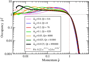
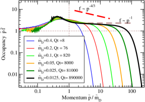
Figure 3: (Left) Evolution of the scaling solution as a function of the screening scale $\tilde{m}_{{}_{\rm{D}}}$ computed using the discrete momentum method. The solutions coincide with each other for ${\tilde{p}}>1$, and exhibit a bump feature at the scale $\tilde{m}_{{}_{\rm{D}}}$. The dashed red line is a fit to the UV part of the spectrum. (Right) The same as Left, but the $x$-axis is scaled so that the screening scale stays at fixed $x=1$ as a function of time. While at early times when $\tilde{m}_{{}_{\rm{D}}}\lesssim 1$, a power-law $\tilde{f}\propto{\tilde{p}}^{\alpha}$ with $\alpha<-1$ may be seen in the data (in particular $\alpha\sim-4/3$ for $\tilde{m}_{{}_{\rm{D}}}\sim 0.1$), at later times when a proper scaling window has emerged, the solution for $\tilde{m}_{{}_{\rm{D}}}<{\tilde{p}}<1$ approaches $\tilde{f}\propto{\tilde{p}}^{-1}$.

6 Summary

In summary, we have considered classical Yang-Mills theory with initial conditions which are statistically isotropic and homogeneous and with the energy residing in the infrared. We have confirmed the existence of a scaling solution for occupancies which obeys $f\sim(Qt)^{\frac{-4}{7}}$ (endowed with a UV scale $p_{\text{max}}\sim Q(Qt)^{\frac{1}{7}}$) by directly solving the Boltzmann equation. The resulting occupancy is in agreement with what has been observed on the lattice over the range of momenta where the approximation of massless kinematics is valid; this is a numerical demonstration of (classical) field-particle duality.

The solution obtained here, however, differs from the lattice findings in the infrared. This is expected, as our kinetic description does not treat infrared excitations as screened. It does not incorporate the Landau cut, nor the dispersion relation of plasmons. These explain the discrepancy at the scale $m_{{}_{\rm D}}$ and below.

The kinetic treatment robustly demonstrates that, at late times when the scales $p_{\rm max}$ and $m_{{}_{\rm D}}$ are well separated, there is not a scaling window where occupancies scale as $p^{-4/3}$, extending down to the scale $m_{{}_{\rm D}}$. Indeed, such behavior would lead to a divergently large rate of change in particle number. However, at intermediate times before a proper scale difference has emerged, the features at scales $m_{{}_{\rm D}}$ and $p_{\rm max}$ combine such that result can be easily misinterpreted — for a limited range in $p$ — as a power law with $f\propto p^{-4/3}$.

It would be interesting to find a way to extend our kinetic treatment to incorporate hard-loop effects for modes of order the screening scale. This may be possible, since the screening scale and the magnetic scale become separated at large $(Qt)$, so the physics at the $m_{{}_{\rm D}}$ scale should be perturbative.

Appendix A ${1\leftrightarrow 2}$ collision integral

Near collinear ${1\leftrightarrow 2}$ splitting processes are, strictly speaking, kinematically not allowed. However, a certain class of higher-order diagrams, like the $2\rightarrow 3$ diagram depicted in Fig. 4, combine and give rise to an effective ${1\leftrightarrow 2}$ process.

2to3amplitude

(50,20) l3,l2,l1r4,r3,r2,r1,r0 $\theta$v2 photon,tension=2l1,v1photon,tension=3v1,v2photonv2,r1photonv2,r2 photon,tension=2l3,v3photonv3,r4photon,label=$q$v1,v3

$\qquad\Longrightarrow\qquad$ (30,20) l3,l2,l1r5,r4,r3,r2,r1,r0,rn1label=$\theta$,label.angle=30v1 photon,tension=3l2,v1photonv1,r1photonv1,r3

Figure 4: $2\rightarrow 3$ processes in the limit where $\theta\sim m_{\text{D}}/p_{\text{max}}$ and $q\sim m_{\text{D}}$ give rise to effective ${1\leftrightarrow 2}$ splittings.

Consider the contribution of ${2\leftrightarrow 3}$ processes to the collision term,

$$\frac{\partial f(p,t)}{\partial t}=\ldots-{\mathcal{C}}_{{2\leftrightarrow 3}}[f(p,t)]\,.$$ (38)

As we have seen, if we consider the external states at fixed energies and angles, the importance of this process declines, relative to the leading-order one, as $(Qt)^{-4/7}$. However, the scattering rate diverges as $\int d^{2}q/q^{4}$, cut off by the soft scale $m_{{}_{\rm D}}$; and even for small $m_{{}_{\rm D}}$ the rate for the process with the extra emitted particle is only down by ${\cal O}(\bar{f})$ relative to the process without it, provided that the particle is emitted at an angle $\theta\mbox{~{}{\raisebox{1.72218pt}{$<$}} {\raisebox{-2.58334pt}{$\sim$}}~{}}q/p$. Therefore the rate for this process, compared to the rate for wide-angle ${2\leftrightarrow 2}$ scattering, is ${\cal O}(\bar{f}/\tilde{m}_{{}_{\rm{D}}}^{2})\sim 1$. But this only occurs in the kinematic range where $q\sim m_{{}_{\rm D}}\ll p$. In this regime, the statistical factors for the “target” particle (the one which does not split) do not matter, $(\tilde{f}^{-1}(k)-\tilde{f}^{-1}(k{+}q))\simeq 0$, and we may simplify the description by only keeping track of the particle which actually undergoes the splitting. Higher-order processes of general form $n\leftrightarrow(n{+}1)$ are also unsuppressed in a similar kinematic region, so that again only the particle which actually undergoes splitting need be directly considered. The contribution to the collision term is AMY5

$${\mathcal{C}}_{{1\leftrightarrow 2}}[f_{p}] = \frac{(2\pi)^{3}}{p^{2}\nu_{g}}\int_{0}^{\frac{p}{2}}dk~{}\gamma^{g}_{gg}(p;k,p-k)\Big{(}f_{p}[1+f_{k}][1+f_{p-k}]-[1+f_{p}]f_{k}f_{p-k}\Big{)}+$$ (39)

$$\frac{(2\pi)^{3}}{p^{2}\nu_{g}}\int_{0}^{\infty}dk~{}\gamma^{g}_{gg}(p+k;p,k)\Big{(}f_{p}f_{k}[1+f_{p+k}]-[1+f_{p}][1+f_{k}]f_{p+k}\Big{)}\,,$$

where the first term represents the possibility that the particle of momentum $p$ should split into (or from) two particles of smaller energy, while the second term represents the production of the particle of momentum $p$ via the splitting of a higher-energy particle (and its inverse process). As before, we make the classical approximation by replacing

$$f_{p}[1+f_{k}][1+f_{p-k}]-[1+f_{p}]f_{k}f_{p-k}\simeq f_{p}f_{k}f_{p-k}\Big{(}f_{k}^{-1}+f_{p-k}^{-1}-f_{p}^{-1}\Big{)}\,.$$ (40)

The splitting kernels $\gamma^{g}_{gg}$ are effective matrix elements for these processes. They were found explicitly in AMY5 , and are given by

$$\gamma^{g}_{gg}(p^{\prime};p,k) = \frac{p^{\prime 4}+p^{4}+k^{4}}{p^{\prime 3}p^{3}k^{3}}\mathcal{F}_{g}(p^{\prime};p,k)$$ (41)

$$\mathcal{F}_{g}(p^{\prime};p,k) = \frac{g^{2}N_{\rm c}\nu_{g}}{4(2\pi)^{4}}\int\frac{d^{2}h}{(2\pi)^{2}}\boldsymbol{h}\cdot\text{Re}\>{\boldsymbol{F}}_{\!\!g}(\boldsymbol{h};p^{\prime},p,k),$$ (42)

where $\boldsymbol{h}=\boldsymbol{p}\times\boldsymbol{k}$ parametrizes the (parametrically small) non-collinearity of the external states, and ${\boldsymbol{F}}_{\!\!g}$ is the solution of the following integral equation,

$$2\boldsymbol{h} = i\delta E(\boldsymbol{h}){\boldsymbol{F}}_{\!\!g}(\boldsymbol{h})$$ (43)

$$\quad+~{}\frac{g^{2}N_{\rm c}T_{*}}{2}\int\frac{d^{2}\boldsymbol{q}}{(2\pi)^{2}}\mathcal{A}(\boldsymbol{q})\big{(}3{\boldsymbol{F}}_{\!\!g}(\boldsymbol{h})-{\boldsymbol{F}}_{\!\!g}(\boldsymbol{h}{-}p\boldsymbol{q})-{\boldsymbol{F}}_{\!\!g}(\boldsymbol{h}{-}k\boldsymbol{q})-{\boldsymbol{F}}_{\!\!g}(\boldsymbol{h}{+}p^{\prime}\boldsymbol{q})\big{)}\qquad$$

with

$$\mathcal{A}(\boldsymbol{q}) = \frac{1}{\boldsymbol{q}^{2}}-\frac{1}{\boldsymbol{q}^{2}+m_{{}_{\rm D}}^{2}}\,,$$ (44)

$$\delta E(\boldsymbol{h}) = \frac{m^{2}_{\text{D}}}{4}\Big{(}\frac{1}{p}+\frac{1}{k}-\frac{1}{p^{\prime}}\Big{)}+\frac{\boldsymbol{h}^{2}}{2pkp^{\prime}}\,,$$ (45)

$$T_{*} = \frac{\int d^{3}p\>{f}^{2}(p)}{\int d^{3}p\>2f(p)/p}.$$ (46)

Now let us determine how these effective ${1\leftrightarrow 2}$ processes scale with $g^{2}N_{\rm c}$ and with time. If we multiply both sides of Eq. (39) by $g^{2}N_{\rm c}$, so it describes the evolution of $\bar{f}$ rather than of $f$, then each factor of $f$ is accompanied by a factor of $g^{2}N_{\rm c}$ and we can write everything in terms of $\bar{f}$. Specifically, the collision term is quadratic in $f$, see Eq. (40); but there are two factors of $g^{2}N_{\rm c}$, the one we just added and the one in the expression for $\mathcal{F}_{g}$, Eq. (42). The factor $g^{2}N_{\rm c}$ in front of $T_{*}$ in Eq. (43) combines with the definition Eq. (46) such that $g^{2}N_{\rm c}T_{*}\equiv\bar{T}_{*}$ is expressed purely in terms of $\bar{f}$. The definition of $m_{{}_{\rm D}}^{2}$, Eq. (11), is also in terms of $\bar{f}$; $m_{{}_{\rm D}}^{2}\sim\bar{f}p_{\rm max}^{2}$. Therefore the factors of $g^{2}N_{\rm c}$ all disappear when we work in terms of $\bar{f}$, just as for ${\mathcal{C}}_{2\leftrightarrow 2}$. This is the same as the statement that ${\mathcal{C}}_{1\leftrightarrow 2}$ has a valid classical limit.

Next we must check how everything scales with time, when $p\sim p_{\rm max}\sim Q(Qt)^{1/7}$ and $\bar{f}\sim(Qt)^{-4/7}$. Because $\bar{T}_{*}\sim p\bar{f}\sim m_{{}_{\rm D}}^{2}/p$, the first and second terms in Eq. (43) are of comparable size when $\boldsymbol{h}\sim m_{{}_{\rm D}}p$, which will be the dominant range for $\boldsymbol{h}$ in Eq. (42). The magnitude of ${\boldsymbol{F}}_{\!\!g}$ is ${\boldsymbol{F}}_{\!\!g}\sim\boldsymbol{h}/\delta E\sim p^{2}/m_{{}_{\rm D}}$, so the integral in Eq. (42) is of order $\left|{\boldsymbol{h}}\right|^{3}{\boldsymbol{F}}_{\!\!g}\sim m_{{}_{\rm D}}^{2}p^{5}$ and $\gamma^{g}_{gg}\sim m_{{}_{\rm D}}^{2}$. By Eq. (11), $m_{{}_{\rm D}}^{2}\sim Q^{2}(Qt)^{\frac{-2}{7}}$, while $p\sim Q(Qt)^{\frac{1}{7}}$ and $\bar{f}\sim(Qt)^{\frac{-4}{7}}$; so the righthand side of Eq. (39) scales as $Q(Qt)^{\frac{-11}{7}}$, exactly the same scaling as the ${2\leftrightarrow 2}$ collision term, see the discussion after Eq. (8).

Eq. (43) is most easily solved by making a transformation to impact parameter space Aurenche ; we introduce

$$\boldsymbol{f}(\boldsymbol{b})=\int\frac{d^{2}q}{(2\pi)^{2}}~{}e^{i\boldsymbol{q}\cdot\boldsymbol{b}}~{}\boldsymbol{f}(\boldsymbol{q}),$$ (47)

and transform Eq. (43) into and ODE (choosing units with $m_{{}_{\rm D}}=1$)

$$-2i\nabla\delta^{(2)}(\boldsymbol{b}) = \frac{i}{2p^{\prime}y(1-y)}\Big{(}\frac{1-y(1-y)}{2}-\nabla^{2}\Big{)}\boldsymbol{f}(\boldsymbol{b})$$ (48)

$$~{}+\frac{g^{2}N_{c}T}{2}\Big{(}D(yb)+D(b-by)+D(b)\Big{)}\boldsymbol{f}(\boldsymbol{b}).$$

In this context, $\boldsymbol{f}(\boldsymbol{q})$ is a re-scaling of the original ${\boldsymbol{F}}_{\!\!g}$, $\boldsymbol{f}(\boldsymbol{q})={\boldsymbol{F}}_{\!\!g}(p^{\prime}\boldsymbol{q})/p^{\prime}$. $p^{\prime}$ is the energy of the incoming gluon, $p^{\prime}=p+k$, by momentum conservation. Hence, $p=(1-y)p^{\prime}$, $k=yp^{\prime}$, where $y$ runs from 0 to 1. The function $D(b)$ is defined by the integral

$$D(b) = \lim_{\epsilon\rightarrow 0}\int\frac{d^{2}q}{(2\pi)^{2}}\frac{1}{(q^{2}+\epsilon^{2})(q^{2}+1)}-e^{i\boldsymbol{q}\cdot\boldsymbol{b}}\frac{1}{(q^{2}+\epsilon^{2})(q^{2}+1)}$$ (49)

$$= \frac{1}{2\pi}\big{(}\gamma_{E}+\log(b/2)+K_{0}(b)\big{)};$$ (50)

$K_{0}$ is a modified Bessel function. Following the procedure laid out in Aurenche and defining $\boldsymbol{f}(\boldsymbol{b})=\boldsymbol{b}h(b)$, we have

$$\mathcal{F}_{g}(p^{\prime};p,k)=\frac{p^{\prime 4}g^{2}N_{\rm c}d_{A}}{2(2\pi)^{4}}\int\frac{d^{2}q}{(2\pi)^{2}}\boldsymbol{q}\cdot\boldsymbol{f}(\boldsymbol{q})=\frac{p^{\prime 4}g^{2}N_{\rm c}d_{A}}{2(2\pi)^{4}}2~{}\text{Im}\lim_{b\rightarrow 0^{+}}h(b).$$ (51)

This limit is obtained via the numerical resolution of the ODE; in practice this quantity only needs to be calculated on some grid of $(p^{\prime},y,T_{*})$ points. When performing the integral in Eq. (13), intermediate values of $\gamma^{g}_{gg}$ are then obtained by interpolation.

The emission and absorption of soft gluons occurs with a divergent rate, but these processes approximately cancel in Eq. (39). In order to make the cancellation explicit, we subdivide $C_{{1\leftrightarrow 2}}[\tilde{f}_{{\tilde{p}}}]$ as follows,

$$C_{{1\leftrightarrow 2}}[\tilde{f}_{{\tilde{p}}}]=C^{A}_{{1\leftrightarrow 2}}[\tilde{f}_{{\tilde{p}}}]+C^{B}_{{1\leftrightarrow 2}}[\tilde{f}_{{\tilde{p}}}]+C^{C}_{{1\leftrightarrow 2}}[\tilde{f}_{{\tilde{p}}}],$$ (52)

where (introducing the tilde variables where the momentum scaling has been incorporated, and absorbing a factor of $8\pi^{2}$ into the definition of $\tilde{\gamma}$)

$$C^{A}_{{1\leftrightarrow 2}}[\tilde{f}_{{\tilde{p}}}] = -\int_{0}^{\frac{{\tilde{p}}}{2}}d\tilde{q}~{}\tilde{\gamma}^{g}_{gg}({\tilde{p}};\tilde{q},{\tilde{p}}-\tilde{q})\Big{(}\tilde{f}_{{\tilde{p}}}\tilde{f}_{\tilde{q}}+\tilde{f}_{{\tilde{p}}}\tilde{f}_{{\tilde{p}}-\tilde{q}}-\tilde{f}_{\tilde{q}}\tilde{f}_{{\tilde{p}}-\tilde{q}}\Big{)}$$ (53)

$$C^{B}_{{1\leftrightarrow 2}}[\tilde{f}_{{\tilde{p}}}] = -\int_{\frac{{\tilde{p}}}{2}}^{\infty}d\tilde{q}~{}\tilde{\gamma}^{g}_{gg}({\tilde{p}}+\tilde{q};{\tilde{p}},\tilde{q})\Big{(}\tilde{f}_{{\tilde{p}}}\tilde{f}_{\tilde{q}}-\tilde{f}_{{\tilde{p}}}\tilde{f}_{{\tilde{p}}+\tilde{q}}-\tilde{f}_{\tilde{q}}\tilde{f}_{{\tilde{p}}+\tilde{q}}\Big{)}$$ (54)

$$C^{C}_{{1\leftrightarrow 2}}[\tilde{f}_{{\tilde{p}}}] = -\int^{\frac{{\tilde{p}}}{2}}_{0}d\tilde{q}~{}\tilde{\gamma}^{g}_{gg}({\tilde{p}}+\tilde{q};{\tilde{p}},\tilde{q})\Big{(}\tilde{f}_{{\tilde{p}}}\tilde{f}_{\tilde{q}}-\tilde{f}_{{\tilde{p}}}\tilde{f}_{{\tilde{p}}+\tilde{q}}-\tilde{f}_{\tilde{q}}\tilde{f}_{{\tilde{p}}+\tilde{q}}\Big{)}.$$ (55)

The sum $C^{A+C}_{{1\leftrightarrow 2}}=C^{A}_{{1\leftrightarrow 2}}+C^{C}_{{1\leftrightarrow 2}}$ is treated by combining the integrands, which makes the cancellations at small $q$ explicit.

Appendix B ${2\leftrightarrow 2}$ collision integral

The ${2\leftrightarrow 2}$ or elastic collision integral we must consider is presented in Eq. (14), Eq. (26), Eq. (4); in addition the matrix element must be modified by the inclusion of hard loops, as described in AMY5 . We perform the integrations using the parametrization of the momentum integrals from AMY5 ,

$$\int\frac{d^{3}pd^{3}kd^{3}p^{\prime}d^{3}k^{\prime}}{(2\pi)^{12}16pkp^{\prime}k^{\prime}}(2\pi)^{4}\delta^{4}(p{+}k{-}p^{\prime}{-}k^{\prime})=\frac{1}{2^{10}\pi^{6}}\int_{0}^{\infty}dq\int_{-q}^{q}d\omega\int_{\frac{q{-}\omega}{2}}^{\infty}dp\int_{\frac{q{+}\omega}{2}}^{\infty}dk\int_{0}^{2\pi}d\phi\,,$$ (56)

with $p^{\prime}=p+\omega$ and $k^{\prime}=k-\omega$. However we want to work at fixed $p$, so we must change the integration order so it is the outermost integral. We also find it convenient to bring the $k$ integral outside the other two and to perform the $q$ integral first;

$$C_{{2\leftrightarrow 2}}[\tilde{f}_{{\tilde{p}}}] = -\frac{1}{2^{9}\pi^{5}}\int_{0}^{\infty}d{\tilde{k}}\int_{-{\tilde{p}}}^{{\tilde{k}}}d\omega~{}f_{{\tilde{p}}}f_{{\tilde{k}}}f_{{\tilde{p}}^{\prime}}f_{{\tilde{k}}^{\prime}}\Big{(}f^{-1}_{{\tilde{p}}^{\prime}}+f^{-1}_{{\tilde{k}}^{\prime}}-f^{-1}_{{\tilde{p}}}-f^{-1}_{{\tilde{k}}}\Big{)}\times$$ (57)

$$\hskip 39.83368pt\int_{\left|{\omega}\right|}^{{\tilde{q}}_{\text{max}}}d\tilde{q}\int_{0}^{2\pi}d\phi~{}\left|\overline{M}^{2}_{{\tilde{p}}{\tilde{k}};{\tilde{p}}^{\prime}{\tilde{k}}^{\prime}}\right|\,,$$

with ${\tilde{q}}_{\text{max}}=\text{min}\{2{\tilde{k}}-\omega,2{\tilde{p}}+\omega\}$. In terms of these variables, the Mandelstam variables $s$ and $t$ appearing in Eq. (4) are

$$s = -\frac{t}{2{\tilde{q}}^{2}}\big{(}(2{\tilde{p}}+\omega)(2{\tilde{k}}-\omega)+{\tilde{q}}^{2}\big{)}+\frac{t}{2{\tilde{q}}^{2}}\sqrt{(4{\tilde{p}}{{\tilde{p}}}^{\prime}+t)(4{\tilde{k}}{{\tilde{k}}}^{\prime}+t)}\cos\phi\,,$$ (58)

$$t = \omega^{2}-{\tilde{q}}^{2}\,.$$ (59)

The main challenge associated with $C_{{2\leftrightarrow 2}}$ is that it contains a 4 dimensional integral that at worst must be entirely computed numerically. Furthermore, for small values of $\tilde{m}_{{}_{\rm{D}}}$, a large array of points is required to achieve a reasonable amount of precision. Eq. (57) is suggestive, in that the distribution functions do not participate in the integrals over $\tilde{q}$ and $\phi$. At best, it may be possible to drastically simplify Eq. (57) by performing the $q,\phi$ integrals analytically. In practice, when we include full hard loops into Eq. (4), the $\phi$ but not the $q$ integral can be done analytically. But we will now show that in the current context we can actually perform the $\tilde{q}$ integral analytically without affecting the reliability of the result.

Note first that the hard loops only play a role for $\omega,\tilde{q}\mbox{~{}{\raisebox{1.72218pt}{$<$}} {\raisebox{-2.58334pt}{$\sim$}}~{}}\tilde{m}_{{}_{\rm{D}}}$. There are two possible cases. Either one or both of ${\tilde{p}},{\tilde{k}}$ are $\mbox{~{}{\raisebox{1.72218pt}{$<$}} {\raisebox{-2.58334pt}{$\sim$}}~{}}\tilde{m}_{{}_{\rm{D}}}$; or ${\tilde{p}},{\tilde{k}}\gg\tilde{m}_{{}_{\rm{D}}}$. In the former case, the hard-loop treatment of the matrix element is anyway not reliable, since we do not account for the modification of the dispersion and spectral weight of the external states. In the latter case, we can Taylor expand the statistical function part of the integrand in small $\omega$. The lowest nontrivial term is ${\cal O}(\omega^{2})$, corresponding to drag and momentum diffusion effects. Higher-order in $\omega$ terms are insensitive to small $q$. Any modification of the matrix element which recovers the same result for the $\omega^{2}$ behavior as the full hard-loop treatment does, is equally accurate.

With this in mind, we make the following substitution in the $t$-channel denominator:

$$\tilde{q}^{2}t\rightarrow t(\tilde{q}^{2}+\xi^{2}\tilde{m}_{{}_{\rm{D}}}^{2})\,.$$ (60)

The $u$-channel case is handled by relabeling external states so that it is the same as the $t$-channel one. With $s$ and $t$ as defined in Eq. (58) and Eq. (59), and the substitution Eq. (60), it is in fact possible to perform the integrals over $\phi$ and $\tilde{q}$ analytically. The parameter $\xi$ is then fixed by performing the above integrals, and the same integrals with the full hard-loop self-energy, and choosing $\xi$ so that the large ${\tilde{p}},{\tilde{k}}$ result, integrated over $\omega^{2}d\omega$, is the same:

$$\mathcal{I}(\xi,\tilde{m}_{{}_{\rm{D}}})=\int_{-\infty}^{\infty}d\omega~{}\omega^{2}\int_{\left|{\omega}\right|}^{\infty}d\tilde{q}\int_{0}^{2\pi}d\phi~{}\left(\left|{\overline{M}^{2}_{\xi,\tilde{m}_{{}_{\rm{D}}}}}\right|^{\text{Approx HTL}}_{{\tilde{k}},{\tilde{p}}\,\gg\tilde{q}}-\left|{\overline{M}^{2}_{\tilde{m}_{{}_{\rm{D}}}}}\right|^{\text{Exact HTL}}_{{\tilde{k}},{\tilde{p}}\,\gg\tilde{q}}\right).$$ (61)

We will therefore obtain the same (integrated) behavior for the regime ${\tilde{p}},{\tilde{k}}\gg\tilde{m}_{{}_{\rm{D}}}$, which is sufficient to ensure that the approach is as accurate as the full hard-loop approach (described and advocated in AMY5 ) within the current context. Numerically we find $\xi=0.83$, which corresponds well with a “sum rule” value of $\xi=e^{5/6}/\sqrt{8}$.

References

- (1) F. Gelis, E. Iancu, J. Jalilian-Marian and R. Venugopalan, The Color Glass Condensate, Ann. Rev. Nucl. Part. Sci. 60 (2010) 463 [arXiv:1002.0333].
- (2) T. Lappi, L. McLerran, Some Features of the Glasma, Nucl. Phys. A 772 (2006) 200 [hep-ph/0602189].
- (3) H. Weigert, Evolution at Small : The Color Glass Condensate, Prog. Part. Nucl. Phys. 55 (2005) 461 [hep-ph/0501087].
- (4) A. Kurkela and G. D. Moore, Thermalization in Weakly Coupled Nonabelian Plasmas, JHEP 12 (2011) 044 [arXiv:1107.5050].
- (5) J.-P. Blaizot et. al., Thermalization and Bose-Einstein Condensation in Overpopulated Glasma, arXiv:hep-ph/1210.6838.
- (6) J. Berges, S. Schlichting and D. Sexty, Over-populated gauge fields on the lattice, Phys. Rev. D 86 (2012) 074006 [arXiv:1203.4646].
- (7) S. Schlichting, Turbulent thermalization of weakly coupled non-abelian plasmas, Phys. Rev. D 86 (2012) 065008 [arXiv:1207.1450]
- (8) A. Kurkela and G. D. Moore, UV Cascade in Classical Yang-Mills Theory, Phys. Rev. D 86 (2012) 056008 [arXiv:1207.1663].
- (9) A. H. Mueller and D. T. Son, On the Equivalence between the Boltzmann equation and classical field theory at large occupation numbers, Phys. Lett. B 582 (2004) 279 [hep-ph/0212198].
- (10) P. Arnold, G. D. Moore and L. G. Yaffe, Effective Kinetic Theory for High Temperature Gauge Theories, JHEP 0301 (2003) 030 [hep-ph/0209353].
- (11) P. Aurenche, F. Gelis, G. D. Moore and H. Zaraket, Landau-Pomeranchuk-Migdal Resummation for Dilepton Production, JHEP 0212 (2002) 006 [hep-ph/0211036].