2D Direction Of Arrival Estimation with Modified Propagator

Abstract

In this paper, a fast algorithm for the Direction Of Arrival (DOA) estimation of radiating sources, based on partial covariance matrix and without eigendecomposition of incoming signals is extended to two dimensional problem of joint azimuth and elevation estimation angles using Uniform Circular Array (UCA) in case of non coherent narrowband signals. Simulation results are presented with both Aditive White Gaussian Noise (AWGN) and real symmetric Toeplitz noise.

1 INTRODUCTION

Estimating the Direction of Arrivals (DOA) of impinging electromagnetic or acoustic waves on antenna array plays a crucial role in many physics and engineering fields such as sonar,radar, astrophysics,Electronic Surveillance Measure (MSE),submarine acoustics, geodesic location , GSM positionnging, geophysics, and so on.

Extensive research has been made in the last two decades leading to an efficient improvement in DOA estimation but every method has its own advantages and disadventages in terms of the nature of environement such as the jamming,reflection, thermal noise, degradation of the antenna elements in the array ,the radiation pattern of the array ,near field scattering and mutual coupling .

A subspace based methods provide high resolution estimation [1],[2], Maximum Likelihood Estimation (ML) and Estimation of Signal Parameters via Rotational Invariance Technique (EPRIT) [3] were proposed in various array geometries such as a Uniform Linear Array (ULA), Uniform Rectangular Array (URA). Howevere the subspace based techniques require extensive computation of the eigendecomposition of covariance matrix of the array output data in order to obtain the sets of signal and noise subspaces, which makes the use of these techniques limited in case of large number of array sensors.

For this reason, a fast DOA estimation methods were proposed [4], [5], [6] without eigendecomposition , the propagation method [7],[8] uses the whole covariance matrix of the output data to obtain the propagation operator but it can be degraded in non uniform colored noise [9] .
To overcome this issue, a modified propoagation method (MPM) [10] were proposed with Uniform Linear Array (ULA) using only partial covariance matrix which makes it lower computationally than the (PM) method [7] and better performing with non Gaussian noise .

In this paper, we present an extension (MPM) method [10] to joint two dimensional azimuth and elevation estimation angles using Uniform Circular Array (UCA) with non moving narrowband radiating sources in both complex Additive White Gaussian Noise (AWGN) and real symmetric Toeplitz noise.

2 DATA MODEL

We consider uniform cicrular array (UCA), consisting of N isotropic and identical antenna elements distributed uniformely over a circle with radius $R=\lambda/2$ with $\lambda$ is the wave length of the impinging electromagnetic waves . The phase azimuth angle of the $n^{th}$ element is $\phi_{n}={{2\pi n}\over{N}}$ with $n=1,2,...,N$ . P narrowband source waves with same carrier frquency $f$ are impinging on the UCA with directions $(\theta_{1},\phi_{1}),(\theta_{2},\phi_{2}),...,(\theta_{P},\phi_{P})$ The received signals can be written in the following form :

$$X(t)=AS(t)+N(t)$$ (1)

Where : $X(t)=[X_{1}(t),X_{2}(t),...,X_{N}(t)]^{T}$ is the $t^{th}$ snapshot of the received signal, $A=[a(\theta_{1},\phi_{1}),a(\theta_{2},\phi_{2}),...,a(\theta_{P},\phi_{P})]$ is the NxP array response with $a(\theta_{m},\phi_{m})=[a_{1}(\theta_{m},\phi_{m}),a_{2}(\theta_{m},\phi_{m}),...a_{N}(\theta_{m},\phi_{m})]^{T}$ is the steering vector from direction $(\theta_{m},\phi_{m})$ where $m=1,2,...,P$, $(\theta_{m},\phi_{m})$ are the elevation and azimuth of the $m^{th}$ signal respectively.$S(t)=[s_{1}(t),s_{2}(t),...,s_{P}(t)]^{T}$ is the source waveform vector and $N(t)=[n_{1}(t),n_{2}(t),...,n_{N}(t)]^{T}$ is the $t^{th}$ snapshot of either zero mean stationary complex additive white Gaussian noise (AWGN) or non uniform spatially and temporally complex colored noise . The steering vector a can be written as the following :
$a_{m}(\theta,\phi)=$

$$e^{2\pi j{R\over\lambda}\left(\sin({\theta})\cos({\phi})\cos({{2\pi m}\over N})+sin({\theta})\sin({\phi})\sin({{2\pi m}\over N})\right)}$$ (2)

Using the goniometric identity $\cos(a\pm b)=\cos(a)\cos(b)\mp\sin(a)\sin(b)$ the steering vector becomes :

$$a_{m}(\theta,\phi)=e^{2\pi j{R\over\lambda}\sin(\theta)\cos({{2\pi m}\over N}-\phi)}$$ (3)

In case of (AWGN) noise the covariance matrix can be written as :

$$R_{xx}=E\{X(t){X(t)^{H}}\}=AR_{ss}A^{H}+\sigma_{N}^{2}I$$ (4)

Where $R_{ss}$ is the covariance matrix of the incident signals , H denotes the hermitian transpose and $I$ is NxN identity matrix .
The angles of arrivals (AOA) can be extracted using $R_{xx}$ when the the following assumptions are respected: (1) The number of sources is known a priori and the number of antenna elements in the UCA satisfies : $N\geqslant 2P+2$.
(2) The P steering vectors are linearly independent and the P signal sources are statistically uncorrelated.
(3) The radiating sources are located in the Fraunhofer field (far field) where the distance of the $m^{th}$ source satisfies $d_{m}\geqslant{2D^{2}\over\lambda}$ where D is the maximal dimension of the UCA elements .

3 THEORY OF THE MODIFIED PROPAGATOR

the Propagator Method (PM) $[7],[8]$ is computationally low because it does not need eigendecomposition of the covariance matrix , but it uses the whole of it, to obtain the propagation operator. When the noise is not stationary ergodic Gaussian, the PM can be degraded $[9]$, to overcome the problem ,we make an extension of the modified version (MPM) $[10]$ on Uniform Circular Array (UCA) as the following :
The array response matrix in equation (3) can be partitionned as the following [10] :

$$A(\theta,\phi)=[A_{1}^{T}(\theta,\phi),A_{2}^{T}(\theta,\phi),A_{3}^{T}(\theta,\phi)]^{T}$$ (5)

The matrices $A_{1}$ and $A_{2}$ have dimensions $P\times P$ where $A_{3}$ is $(N-2P)\times P$. Based on the equation (1) and the above partition, we can extract the following partial cross correlation matrices from $R_{xx}$ :

$$R_{12}=E\{X_{t}[1:P,:]X_{t}^{H}[P+1:2P,:]\}=A_{1}R_{ss}A_{2}^{H}$$ (6)

$$R_{31}=E\{X_{t}[2P+1:N,:]X_{t}^{H}[1:P,:]\}=A_{3}R_{ss}A_{1}^{H}$$ (7)

$$R_{32}=E\{X_{t}[2P+1:N,:]X_{t}^{H}[P+1:2P,:]\}=A_{3}R_{ss}A_{2}^{H}$$ (8)

The matrices $A_{i}$, $i=(1,2)$ and Rss are full rank according the assumption 2, therefore we can compute the matrix $A_{3}$ with two different ways :

$$R_{32}R_{12}^{-1}A_{1}=A_{3}R_{ss}A_{2}A_{2}^{-H}R_{ss}^{-1}A_{1}^{-1}A_{1}=A_{3}$$ (9)

$$R_{31}R_{21}^{-1}A_{2}=A_{3}R_{ss}A_{1}A_{1}^{-H}R_{ss}^{-1}A_{2}^{-1}A_{2}=A_{3}$$ (10)

Combining equations (14) and (15) gives :

$$R_{32}R_{12}^{-1}A_{1}+R_{31}R_{21}^{-1}A_{2}=2A_{3}$$ (11)

Augmenting the left hand side of the equation (16) yields to :

$$\left[R_{32}R_{12}^{-1}\hskip 14.22636ptR_{31}R_{21}^{-1}\hskip 14.22636pt-2I_{N-2P}\right]A=0$$ (12)

which is equivalent to :

$$Q^{H}A=0$$ (13)

When the P signals are registered with corresponding directions $(\theta_{k},\phi_{k})$ the equation (18) holds :

$$Q^{H}a(\theta_{k},\phi_{k})=0\hskip 56.9055ptk=1,2,...P$$ (14)

Finally when scanning the azimuth and elevation angles in the ranges $[0,2\pi]$ $[0,{\pi\over{2}}]$ respectively, the two dimensional spatial spectrum has peaks when encountring the true signals directions :

$$f(\theta,\phi)={1\over{{\|Q^{H}a(\theta,\phi)\|}^{2}}}$$ (15)

Where the steering vector a is defined by :

$$a(\theta_{i},\phi_{i})=\left[e^{z_{i}\cos(\phi_{i})},e^{z_{i}\cos(\phi_{i}-{2\pi\over N})},...,e^{z_{i}\cos(\phi_{i}-{2\pi(N-1)\over N})}\right]$$ (16)

where $z_{i}=2\pi j{R\over\lambda}\sin(\theta_{i})$, $(\theta_{i},\phi_{i})$ are the $i^{th}$ scanned angles with $\theta_{i}\in\left[0:{1\over f_{\theta}}:{\pi\over 2}\right]$,$\phi_{i}\in\left[0:{1\over f_{\phi}}:2\pi\right]$ , $(f_{\theta},f_{\phi})$ are the desired spatial sampling frequencies .

4 RESULTS AND DISCUSSION

We consider a Uniform Circular Array (UCA) consisting of $N=14$ identical dipoles elements having the same exitation and zero phase, with operation frequency $f=900MHz$, the radius of the UCA is $R=38cm$ with interlement spacing $d=16cm$ as illustrated in the figure 1.
Three non coherent and almost equipowered narrowband sources are impinging on the array from $(\theta_{1}=15^{\circ},\phi_{1}=20^{\circ})$,$(\theta_{2}=30^{\circ},\phi_{2}=44^{\circ})$ and $(\theta_{3}=66^{\circ},\phi_{3}=69^{\circ})$ respectively with $K=100$ snapshots .

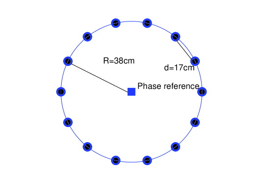
Figure 1: UCA, $d=\lambda/2$.

The figure 1 represents the average of $L=50$ Monte Carlo simulation trials when the $SNR=10dB$.

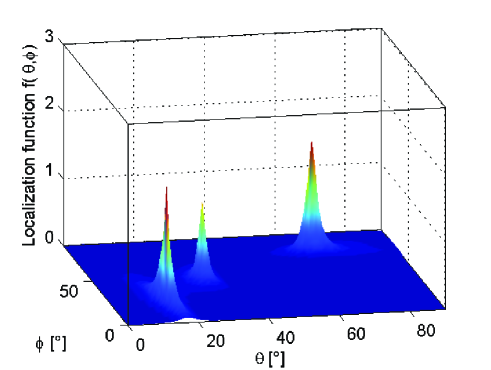
Figure 2: Modified Propagator, $SNR=10dB$.

In the second simulation, we evaluated the (MPM) in case of real symmetric Toeplitz noise where the noise covariance is given by :

$$Rn=Toeplitz([1,0.93,0.86,...,0.1])$$ (17)

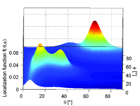
Figure 3: Modified Propagator in real symmetric toeplitz noise

The MPM method can be succeful in the presence of non uniform noise . The advantage of the modified propagator is complexity[10], while the high resolution MUSIC algorithm involves $N^{2}K$ for computing the covariance matrix $R_{xx}$ and $O(N^{3})$ for its Eigen-Value Decomposition (EVD), and the number of floating points the (PM) method takes for computing the propagator Q is $NPK+O(P^{3})$ , the MPM algorithm only involves $P(N-P)K+O(P^{3})$.
If the sources are correlated or coherent to each other, the algorithm will fail to detect the DOAs, to get the same result one needs to use preprocessing techniques on the covariance matrix such as the Forward Backward Averaging (FBA) or the spatial smoothing.

5 Conclusion

A Modified Propagator Method (MPM) for DOA estimation has been extended to two dimensional azimuth and elevation angles using Uniform Circular Array (UCA), the partial cross correlation matrices are used to compute the propagation operator using off diagonals of the output cross correlation matrix, hence the MPM is suitable to the case of non uniform noise which is confirmed by simulation in the presence of real symmetric Toeplitz noise .

References

-
[1]
R. O. Schmidt, Multiple Emitter Location and Signal Parameter Estimation, IEEE Transactions on Antennas and Propagation, Vol. 34, No. 3, 1986, pp. 276-280.
-
[2]
B. D. Rao and K. V. S. Hari, Performance Analysis of Root-Music, IEEE Transactions on Acoustics, Speech and Signal Processing, Vol. 37, No. 12, 1989, pp. 1939-1949.
-
[3]
R. Roy and T. Kailath, ESPRIT-Estimation of Signal Parameters via Rotational Invariance Techniques, IEEE Transactions on Acoustics, Speech and Signal Processing, Vol. 37, No. 17, 1989, pp. 984-995.
- [4] M. Frikel, LOCALIZATION OF SOURCES RADIATING ON A LARGE ANTENNA . 13th European Signal processing conference, 4-8 september 2005 ( EUSIPCO 2005).
- [5] J. Xin and A. Sano, Computationally Efficient Subspace Based Method for Direction of Arrival Estimation with-out Eigendecomposition, IEEE Transactions on Signal Processing, Vol. 52, No. 4, 2004, pp. 876-893.
-
[6]
J. F. Gu, P. Wei and H. M. Tai, Fast Direction-of-Arrival Estimation with Known Waveforms and Linear Opera-tors, IET Signal Processing, Vol. 2, No. 1, 2008, pp. 27-36.
-
[7]
S. Marcos, A. Marsal and M. Benidir, The Propagator Method for Source Bearing Estimation, Signal Process-ing, Vol. 42, No. 2, 1995, pp. 121-138.
-
[8]
J. Munier and G. Y. Delisle, Spatial Analysis Using New Properties of the Cross-Spectral Matrix, IEEE Transac-tions on Signal Processing, Vol. 39, No. 3, 1991, pp. 746-749.
-
[9]
Y. T. Wu, C. H. Hou, G. S. Liao and Q. H. Guo, Direc-tion of Arrival Estimation in the Presence of Unknown Nonuniform Noise Fields, IEEE Journal of Oceanic En-gineering, Vol. 31, No. 2, 2006, pp. 504-510.
- [10] Jianfeng Chen, Yuntao Wu, Hui Cao, Hai Wang , Fast Algorithm for DOA Estimation with Partial Covariance Matrix and without Eigendecomposition , Journal of Signal and information Processing, 2011,2,266-259. Published Online November 2011 ,SciRes.
- [11] Safi, S. and Zeroual, A. and Hassani, M. Prediction of global daily solar radiation using higher order statistics ,Renewable Energy, 2002.ELSVIER.
- [12] M. Frikel,B. Targui,S. Safi and M. M saad,”Bearing detection of noised wideband sources for geolocation”.18th Mediterranean Conference on Control and Automation (MED),23-25 June 2010, page :1650-1653.
- [13] S. Ejaz and M. A. Shafiq, ”COMPARISON OF SPECTRAL AND SUBSPACE ALGORITHMS FOR FM SOURCE ESTIMATION”, Progress in Electromagnetic Research C, Vol.14,11-21,2010.
- [14] M. Frikel, ”LOCALIZATION OF SOURCES RADIATING ON A LARGE ANTENNA”. 13th European Signal processing conference, 4-8 september 2005 ( EUSIPCO 2005).
- [15] Ping TAN, ”Study of 2D DOA Estimation for Uniform Circular Array in Wireless Location System”, I.J. Computer Network and Information Security,Published Online December 2010 in MECS.
- [16] Lutao Liu C Qingbo Ji CYilin Jiang, ”Improved Fast DOA Estimation Based on Propagator Method”, APSIPA ASC 2011 Xi an.