Reweighted $l_{1}$-norm Penalized LMS for Sparse Channel Estimation and Its Analysis

Abstract

A new reweighted $l_{1}$-norm penalized least mean square (LMS) algorithm for sparse channel estimation is proposed and studied in this paper. Since standard LMS algorithm does not take into account the sparsity information about the channel impulse response (CIR), sparsity-aware modifications of the LMS algorithm aim at outperforming the standard LMS by introducing a penalty term to the standard LMS cost function which forces the solution to be sparse. Our reweighted $l_{1}$-norm penalized LMS algorithm introduces in addition a reweighting of the CIR coefficient estimates to promote a sparse solution even more and approximate $l_{0}$-pseudo-norm closer. We provide in depth quantitative analysis of the reweighted $l_{1}$-norm penalized LMS algorithm. An expression for the excess mean square error (MSE) of the algorithm is also derived which suggests that under the right conditions, the reweighted $l_{1}$-norm penalized LMS algorithm outperforms the standard LMS, which is expected. However, our quantitative analysis also answers the question of what is the maximum sparsity level in the channel for which the reweighted $l_{1}$-norm penalized LMS algorithm is better than the standard LMS. Simulation results showing the better performance of the reweighted $l_{1}$-norm penalized LMS algorithm compared to other existing LMS-type algorithms are given.

1 Introduction

The least mean square (LMS) algorithm is very well known in the field of adaptive signal processing [1], [2]. It belongs to the class of stochastic gradient algorithms. The attractive feature of the LMS algorithm is that it does not need extensive stochastic knowledge of the channel and the input data sequence unlike some other parameter estimation methods such as the recursive least squares (RLS) and Kalman filter. While RLS and Kalman filter need to know the covariance matrix of the input data sequence, the LMS algorithm only requires an approximate estimate of the largest eigenvalue of the covariance matrix for proper selection of the step size that guarantees the convergence. The LMS algorithm is being employed in a wide variety of applications in signal processing and communications including system identification [3], echo cancellation [4], channel estimation [5], adaptive communication line enhancement [6], etc. A particular application considered in this paper is that of estimating a finite impulse response (FIR) channel. The choice of the channel estimation algorithm for use in a communication system comes down to the available information about the statistics of the system, the desired performance of the estimation algorithm, as well as the complexity of the estimation process.

The standard recursive parameter estimation algorithms do not assume any information about the specific structure of the channel being estimated. However, being aware of the channel structure one can modify the standard algorithms in order to have a better estimate of the channel. In this paper, we are concerned with a class of channels where the channel impulse response (CIR) is sparse. A time sparse discrete-time signal is the one with only a few nonzero entries. In general, the domain that the signal is sparse in does not necessarily have to be the time domain. Other sparsity bases can also be used and are represented by an $N\times N$ orthogonal matrix where $N$ is the length of the signal.

Sparsity-aware modifications of the LMS algorithm have been presented in the signal processing literature in the past few years. The methods introduced in [7], [8] add a penalty term to the standard LMS error function which is designed in a way to force the solution to be sparse. A penalty in the form of the $l_{0}$-pseudo-norm of the CIR is used in [8], while [7] uses the $l_{1}$-norm. In [9], the mean square convergence and stability analysis for one of the algorithms in [7] for the case of white input signals is presented. A performance analysis of the $l_{0}$-pseudo-norm constraint LMS algorithm of [8] is given in [10]. In [11], [12], variations of the algorithms in [7] are introduced. In [11], the filter coefficients are updated in a transform domain which leads to faster convergence for non white inputs. In [13], the idea of using a weighted $l_{1}$-norm penalty for the purpose of sparse system identification is presented without any convergence analysis. Moreover, sparsity promoting partial update LMS algorithms have been recently developed in [14].

The authors of [15] introduce a scheme that employs two sequential adaptive filters for communication line or network echo cancelers. The method exploits the sparseness of the CIR and uses two sequential LMS type structures which are both shorter than the largest delay of the channel. A family of the so called natural gradient estimation algorithms is also studied in [16]. It is shown that the class of sparse LMS algorithms presented has faster convergence rate.

Sparse diffusion schemes are presented in [17] and [18] that provide adaptive algorithms for distributed learning in networks. In [17], projection methods over hyperslabs and weighted $l_{1}$-balls are presented and analyzed for distributed learning. Penalized cost functions are used in [18] to enforce the sparsity of the solution. Among the penalty terms considered is the weighted $l_{1}$-norm penalty of [7]. Convergence analysis for the distributed adaptive algorithm is also given in [18] for a convex penalty term.

Other channel estimation algorithms have also been modified to either better adapt to a sparse channel or achieve the same performance as the corresponding standard algorithms with lower complexity. Time and norm-weighted least absolute shrinkage and selection operator (LASSO) where weights obtained from RLS algorithm has been presented in [19]. A greedy RLS algorithm designed for finding sparse solutions to linear systems has been presented in [20], and it has been demonstrated that it has better performance than the standard RLS algorithm for estimating sparse time-varying FIR channels. A compressed sensing (CS)-based Kalman filter has been developed in [21] for estimating signals with time varying sparsity pattern.

In this paper, we first derive the reweighted $l_{1}$-norm penalized LMS algorithm which is based on modifying the LMS error (objective) function by adding the $l_{1}$-norm penalty term and also introducing a reweighting of the CIR coefficients. Then the main contribution follows that is the in depth study of the convergence and excess mean square error (MSE) analysis of the reweighted $l_{1}$-norm penalized LMS algorithm. It is worth mentioning that the analytic arguments in [18] can be applied to a centralized learning problem as well as a diffusion network. In this way, it is also possible to prove the mean square stability of the reweighted $l_{1}$-norm penalized LMS algorithm in a different manner than presented in this paper. Our simulation results show that the proposed algorithm outperforms the standard LMS as well as the penalized sparsity-aware LMS algorithms of [7] and approve our theoretical studies.

The rest of the paper is organized as follows. Section 2 reviews the system model used and the standard LMS algorithm. In Section 3, the reweighted $l_{1}$-norm penalized LMS algorithm is introduced. An analytical study of the convergence of the reweighted $l_{1}$-norm penalized LMS algorithm as well as its excess MSE is given in Section 4. Simulation results comparing the performance of different sparsity-aware LMS algorithms are given in Section 5. Section 6 concludes the paper.

2 System Model and Preliminaries

2.1 Standard LMS

The standard LMS algorithm is used to estimate the actual CIR of a system where the CIR vector denoted as $\boldsymbol{w}$. Let us introduce as well other notations that we need in the following. An estimate of the actual CIR vector $\boldsymbol{w}$ at the time step $k$ is denoted as $\boldsymbol{w}_{k}$. The system’s input data vector is $\boldsymbol{x}_{k}$, $n_{k}$ stands for the additive noise, $d_{k}$ is the desired response of a system, and $e_{k}$ is the error signal. The CIR is assumed to be of length $N$, and therefore, $\boldsymbol{w}\triangleq[w_{1}\;w_{2}\;\cdots\;w_{N}]^{T}$, $\boldsymbol{w}_{k}\triangleq[w_{1,k}\;w_{2,k}\;\cdots\;w_{N,k}]^{T}$, and $\boldsymbol{x}_{k}\triangleq[x_{k}\;x_{k-1}\;\cdots\;x_{k-N+1}]^{T}$, where $(\cdot)^{T}$ stands for the vector transposition. As shown in Fig. LABEL:fig:comsystemmodel

$$d_{k}=\boldsymbol{w}^{T}\boldsymbol{x}_{k}+n_{k}$$

$$e_{k}\triangleq d_{k}-\boldsymbol{w}^{T}_{k}\boldsymbol{x}_{k}.$$ (1)

The noise samples $n_{k}$ are assumed to be independent and identically distributed (i.i.d.) with zero mean and variance of $\sigma^{2}_{\rm n}$. Also, the input data sequence $\boldsymbol{x}_{k}$ and the additive noise samples $n_{k}$ are assumed to be independent.

In standard LMS, the cost function is $L_{k}\triangleq(1/2)e^{2}_{k}$, and it is minimized using the gradient descent algorithm [1]. The update equation of the standard LMS algorithm can be derived from the above mentioned cost function as

$$\boldsymbol{w}_{k+1}=\boldsymbol{w}_{k}-\mu\frac{\partial L_{k}}{\partial\boldsymbol{w}_{k}}=\boldsymbol{w}_{k}+\mu e_{k}\boldsymbol{x}_{k}$$ (2)

where $\mu$ is the step size of the iterative algorithm. To make sure that the LMS algorithm converges, $\mu$ is chosen such that $0<\mu<\lambda^{-1}_{\rm max}$ with $\lambda_{\rm max}$ being the maximum eigenvalue of the covariance matrix of $\boldsymbol{x}_{k}$, i.e., $\boldsymbol{R}\triangleq E\big{[}\boldsymbol{x}_{k}\boldsymbol{x}^{T}_{k}\big{]}$. For the purpose of convergence analysis of the LMS algorithm, a coefficient error vector is usually defined as

$$\boldsymbol{v}_{k}\triangleq\boldsymbol{w}_{k}-\boldsymbol{w}.$$ (3)

The data vector $\boldsymbol{x}_{k}$ is assumed to be independent of the coefficient error vector $\boldsymbol{v}_{k}$. The excess MSE denoted as $\xi_{k}$ is defined as $\xi_{k}\triangleq E\big{[}\left(\boldsymbol{v}^{T}_{k}\boldsymbol{x}_{k}\right)^{2}\big{]}$. It can be further expanded as

$$\xi_{k}=E\big{[}\boldsymbol{v}^{T}_{k}\boldsymbol{x}_{k}\boldsymbol{x}^{T}_{k}\boldsymbol{v}_{k}\big{]}.$$ (4)

In (4), $\boldsymbol{v}^{T}_{k}\boldsymbol{x}_{k}\boldsymbol{x}^{T}_{k}\boldsymbol{v}_{k}$ is a scalar, and therefore, it is equal to its trace, denoted hereafter as $\text{ tr}\{\cdot\}$. Also, since $\text{ tr}\left\{\boldsymbol{v}^{T}_{k}\boldsymbol{x}_{k}\boldsymbol{x}^{T}_{k}\boldsymbol{v}_{k}\right\}=\text{ tr}\left\{\boldsymbol{x}_{k}\boldsymbol{x}^{T}_{k}\boldsymbol{v}_{k}\boldsymbol{v}^{T}_{k}\right\}$ and the two mathematical operators of matrix trace and expectation are interchangeable we can simplify (4) as

$$\xi_{k}=E\big{[}\text{ tr}\left\{\boldsymbol{v}^{T}_{k}\boldsymbol{x}_{k}\boldsymbol{x}^{T}_{k}\boldsymbol{v}_{k}\right\}\big{]}=\text{ tr}\left\{\boldsymbol{R}E\big{[}\boldsymbol{v}_{k}\boldsymbol{v}^{T}_{k}\big{]}\right\}.$$ (5)

Let us introduce the matrix $\boldsymbol{R_{v}}\triangleq\lim_{k\to\infty}E\big{[}\boldsymbol{v}_{k}\boldsymbol{v}^{T}_{k}\big{]}$ and the vector $\xi\triangleq\lim_{k\to\infty}\xi_{k}$. Then we have from (5) that $\xi=\text{tr}\left\{\boldsymbol{R}\boldsymbol{R_{v}}\right\}$. Moreover, the excess MSE can be found as [7]

$$\xi=\frac{\eta}{2-\eta}\sigma^{2}_{\rm n}$$ (6)

where

$$\eta\triangleq\mu\text{ tr}\left\{\boldsymbol{R}\left(\boldsymbol{I}-\mu\boldsymbol{R}\right)^{-1}\right\}.$$ (7)

3 Reweighted $l_{1}$-norm Penalized LMS Algorithm

In the standard LMS algorithm, the fact that the cost function is convex guarantees that the gradient descent algorithm converges to the optimum point under the aforementioned condition on $\mu$. The standard LMS algorithm assumes no structural information about the signal/system to be estimated. Taking any structural information into account, one should be able to modify the algorithm and benefit by lower estimation error, faster convergence, or lower algorithm complexity. In this paper, we are interested in the case when the CIR is sparse. For a CIR $\boldsymbol{w}$ to be sparse in some sparsity domain $\boldsymbol{\Psi}$ most of the coefficients in the vector representation of $\boldsymbol{w}$ in this domain $\boldsymbol{\Psi}$ should be zeros or insignificant in value. Several sparsity-aware modifications of the standard LMS have been introduced in the literature [7, 8, 9, 10, 11, 12, 13, 24].

The reweighted $l_{1}$-norm minimization for sparse signal recovery has a better performance than the standard $l_{1}$-norm minimization that is usually employed in the CS literature [25]. It is due to the fact that a properly reweighted $l_{1}$-norm approximates the $l_{0}$-pseudo-norm, which actually needs to be minimized, better than the $l_{1}$-norm. Therefore, one approach to enforce the sparsity of the solution for the sparsity-aware LMS-type algorithms is to introduce the reweighted $l_{1}$-norm penalty term in the cost function [24]. Our reweighted $l_{1}$-norm penalized LMS algorithm considers a penalty term proportional to the reweighted $l_{1}$-norm of the coefficient vector. The corresponding cost function can be written as

$$L^{\rm rl_{1}}_{k}\triangleq(1/2)e^{2}_{k}+\gamma_{\rm r}\|\boldsymbol{s}_{k}\boldsymbol{w}_{k}\|_{1}$$ (8)

where $\|\cdot\|_{1}$ stands for the $l_{1}$-norm of a vector and $\gamma_{\rm r}$ is the weight associated with the penalty term and elements of the $1\times N$ row vector $\boldsymbol{s}_{k}$ are set to

$$[\boldsymbol{s}_{k}]_{i}=\frac{1}{\epsilon_{\rm r}+|[\boldsymbol{w}_{k-1}]_{i}|},\;\;\;\;i=1,\ldots,N$$ (9)

with $\epsilon_{\rm r}$ being some positive number. The update equation can be derived by differentiating (8) with respect to the vector of CIR coefficients and using the gradient descent principle shown in (2). The resulting update equation is

$$\boldsymbol{w}_{k+1}=\boldsymbol{w}_{k}+\mu e_{k}\boldsymbol{x}_{k}-\rho_{\rm r}\frac{\text{sgn}(\boldsymbol{w}_{k})}{\epsilon_{\rm r}+|\boldsymbol{w}_{k-1}|}$$ (10)

where $\rho_{\rm r}=\mu\gamma_{\rm r}$ and $\text{sgn}(\cdot)$ is the sign function which operates on every component of the vector separately and it is zero for $x=0$, $1$ for $x>0$, and $-1$ for $x<0$. The absolute value operator as well as the $\text{sgn}(\cdot)$ and the division operator in the last term of (10) are all component-wise. Therefore, the $i$-th element of $\text{sgn}(\boldsymbol{w}_{k})/\left(\epsilon_{\rm r}+|\boldsymbol{w}_{k-1}|\right)$ is $[\text{sgn}(\boldsymbol{w}_{k})]_{i}/\left(\epsilon_{\rm r}+|[\boldsymbol{w}_{k-1}]_{i}|\right)$. Note that although the weight vector $\boldsymbol{s}_{k}$ changes in every stage of this sparsity-aware LMS algorithm, it does not depend on $\boldsymbol{w}_{k}$, and the cost function $L^{\rm rl_{1}}_{k}$ is convex. Therefore, the reweighted $l_{1}$-norm penalized LMS algorithm is guaranteed to converge to the global minimum under some conditions. Thus, we study the convergence of the proposed algorithm in the next section.

4 Convergence Study of the Reweighted $l_{1}$-norm Penalized LMS Method

The reweighted $l_{1}$-norm penalized LMS algorithm follows the logic that the penalty term resembling the $l_{0}$-pseudo-norm of the coefficient vector forces the solution of the modified LMS algorithm to be sparse. The cost function of the reweighted $l_{1}$-norm penalized LMS algorithm is given in (8), while the update equation is given in (10).

4.1 Mean Convergence

We first study the mean convergence of the reweighted $l_{1}$-norm penalized LMS algorithm. The update equation for the coefficient error vector of the $l_{1}$-norm penalized LMS $\boldsymbol{v}_{k}$ can be written as

$$\boldsymbol{v}_{k+1} =\boldsymbol{v}_{k}+\mu\big{(}(\boldsymbol{w}^{T}-\boldsymbol{w}^{T}_{k})\boldsymbol{x}_{k}+n_{k}\big{)}\boldsymbol{x}_{k}-\rho_{\rm r}\frac{\text{sgn}(\boldsymbol{w}_{k})}{\epsilon_{\rm r}+|\boldsymbol{w}_{k-1}|}$$

$$=\boldsymbol{v}_{k}-\mu\boldsymbol{v}^{T}_{k}\boldsymbol{x}_{k}\boldsymbol{x}_{k}+\mu n_{k}\boldsymbol{x}_{k}-\rho_{\rm r}\frac{\text{sgn}(\boldsymbol{w}_{k})}{\epsilon_{\rm r}+|\boldsymbol{w}_{k-1}|}.$$ (11)

Since $\boldsymbol{v}^{T}_{k}\boldsymbol{x}_{k}$ is a scalar which is equal to $\boldsymbol{x}^{T}_{k}\boldsymbol{v}_{k}$, (4.1) can be rewritten as

$$\boldsymbol{v}_{k+1}=\boldsymbol{v}_{k}-\mu\boldsymbol{x}_{k}\boldsymbol{x}^{T}_{k}\boldsymbol{v}_{k}+\mu n_{k}\boldsymbol{x}_{k}-\rho_{\rm r}\frac{\text{sgn}(\boldsymbol{w}_{k})}{\epsilon_{\rm r}+|\boldsymbol{w}_{k-1}|}.$$ (12)

From (12) we can derive the evolution equation for $E\big{[}\boldsymbol{v}_{k}\big{]}$. Since $n_{k}$ and $\boldsymbol{x}_{k}$ are independent and $n_{k}$ is assumed to have zero mean, we have $E\big{[}\mu n_{k}\boldsymbol{x}_{k}\big{]}=0$. Then the evolution equation is

$$E\big{[}\boldsymbol{v}_{k+1}\big{]}=\left(\boldsymbol{I}-\mu\boldsymbol{R}\right)E\big{[}\boldsymbol{v}_{k}\big{]}-\rho_{\rm r}E\bigg{[}\frac{\text{sgn}(\boldsymbol{w}_{k})}{\epsilon_{\rm r}+|\boldsymbol{w}_{k-1}|}\bigg{]}.$$ (13)

It is easy to see that the term $\text{sgn}(\boldsymbol{w}_{k})/(\epsilon_{\rm r}+|\boldsymbol{w}_{k-1}|)$ is bounded below and above element-wise as follows

$$\frac{-\boldsymbol{1}}{\epsilon_{\rm r}}\leq\frac{\text{sgn}(\boldsymbol{w}_{k})}{\epsilon_{\rm r}+|\boldsymbol{w}_{k-1}|}\leq\frac{\boldsymbol{1}}{\epsilon_{\rm r}}$$ (14)

where $\boldsymbol{1}$ is the vector with all of its entries set to one. Indeed, $-1$ is always less than or equal to $\text{sgn}(\boldsymbol{w}_{k})$, while $1$ is always larger than or equal to $\text{sgn}(\boldsymbol{w}_{k})$. Moreover, $|\boldsymbol{w}_{k-1}|$ and $\epsilon_{\rm r}$ are always non-negative, which means that the denominator of the middle term in (14) is always larger than or equal to the denominator of the right and left terms of (14), which means that (14) always holds true.

We can further see that, $\rho_{\rm r}E\big{[}\text{sgn}(\boldsymbol{w}_{k})/\left(\epsilon_{\rm r}+|\boldsymbol{w}_{k-1}|\right)\big{]}$ is bounded between $(-\rho_{\rm r}/\epsilon_{\rm r})\boldsymbol{1}$ and $(\rho_{\rm r}/\epsilon_{\rm r})\boldsymbol{1}$. This bound on the second term on the right hand side of (14) is helpful for studying the mean convergence of the reweighted $l_{1}$-norm penalized LMS algorithm. The following theorem establishes our main result on the mean convergence of the reweighted $l_{1}$-norm penalized LMS algorithm.

Theorem 1.

If the maximal eigenvalue of the matrix $\boldsymbol{I}-\mu\boldsymbol{R}$ is smaller than 1, then the mean coefficient error vector $E\big{[}\boldsymbol{v}_{k}\big{]}$ is bounded as $k\to\infty$.

Let $\boldsymbol{Q}\boldsymbol{\Lambda}\boldsymbol{Q}^{T}$ be the eigenvalue decomposition of $\boldsymbol{R}$. Equation (13) can be rewritten as

$$E\big{[}\boldsymbol{c}_{k+1}\big{]}=\left(\boldsymbol{I}-\mu\boldsymbol{\Lambda}\right)E\big{[}\boldsymbol{c}_{k}\big{]}-\boldsymbol{w}^{\prime}_{k}$$ (15)

where

$$\boldsymbol{c}_{k}\!\! \triangleq \!\!\boldsymbol{Q}^{T}\boldsymbol{v}_{k}$$

$$\boldsymbol{w}^{\prime}_{k}\!\! \triangleq \!\!\rho_{\rm r}\boldsymbol{Q}^{T}E\bigg{[}\frac{\text{sgn}(\boldsymbol{w}_{k})}{\epsilon_{\rm r}+|\boldsymbol{w}_{k-1}|}\bigg{]}.$$ (16)

Let also $\boldsymbol{q}$ be the vector whose $i$-th entry is the sum of the absolute values of the elements in the $i$-th row of the matrix $\boldsymbol{Q}^{T}$. The variable $q_{m}$ is defined as the maximum element of the vector $\boldsymbol{q}$. The vector $\boldsymbol{Q}^{T}\text{sgn}(\boldsymbol{w}_{k})$ is thus bounded between $q_{m}\boldsymbol{1}$ and $-q_{m}\boldsymbol{1}$. Therefore, the variable $\boldsymbol{w}^{\prime}_{k}$ in (16) is bounded between $(\rho_{\rm r}q_{m}/\epsilon_{\rm r})\boldsymbol{1}$ and $(-\rho_{\rm r}q_{m}/\epsilon_{\rm r})\boldsymbol{1}$.

It is easy to see from (15) that

$$E\big{[}\boldsymbol{c}_{k+M}\big{]}\!\! = \!\!\left(\boldsymbol{I}-\mu\boldsymbol{\Lambda}\right)^{M}E\big{[}\boldsymbol{c}_{k}\big{]}$$ (17)

$$\quad-\sum_{m=0}^{M-1}{\left(\boldsymbol{I}-\mu\boldsymbol{\Lambda}\right)^{m}\boldsymbol{w}^{\prime}_{k+M-m-1}}.$$

Moreover, since $\boldsymbol{\Lambda}$ and correspondingly $\boldsymbol{I}-\mu\boldsymbol{\Lambda}$ are diagonal matrices, the convergence behavior of every element of the vector $E\big{[}\boldsymbol{c}_{k+M}\big{]}$ can be studied separately.

Let $\lambda_{i}$ be the $i$-th diagonal element of the matrix $\boldsymbol{\Lambda}$. From (17), we have

$$\bigg{[}E\big{[}\boldsymbol{c}_{k+M}\big{]}\bigg{]}_{i} =\left(1-\mu\lambda_{i}\right)^{M}\bigg{[}E\big{[}\boldsymbol{c}_{k}\big{]}\bigg{]}_{i}$$

$$\;\;\;\;-\sum_{m=0}^{M-1}{\left(1-\mu\lambda_{i}\right)^{m}\bigg{[}\boldsymbol{w}^{\prime}_{k+M-m-1}\bigg{]}_{i}}$$ (18)

where $[\cdot]_{i}$ denotes the $i$-th entry of a vector. Since the largest eigenvalue of $\boldsymbol{I}-\mu\boldsymbol{R}$ is smaller than 1, then all the diagonal elements $1-\mu\lambda_{i}$ are smaller than 1. Also note that the $i$-th entry of the vector $\boldsymbol{w}^{\prime}_{k}$ is bounded between $\rho_{\rm r}q_{m}/\epsilon_{\rm r}$ and $-\rho_{\rm r}q_{m}/\epsilon_{\rm r}$. Therefore, by letting $M\to\infty$, the sum on the right hand side of (4.1) is a geometric series with a common ratio of $1-\mu\lambda_{i}$ and is bounded between $\rho_{\rm r}q_{m}/(\mu\lambda_{i}\epsilon_{\rm r})$ and $-\rho_{\rm r}q_{m}/(\mu\lambda_{i}\epsilon_{\rm r})$. The other term on the right hand side of (4.1) approaches zero as $M\to\infty$. As a result, $\bigg{[}E\big{[}\boldsymbol{c}_{k+M}\big{]}\bigg{]}_{i}$ as well as the whole vector $E\big{[}\boldsymbol{c}_{k+M}\big{]}$ are bounded when $M\to\infty$. Since according to (16) $E\big{[}\boldsymbol{c}_{k}\big{]}$ is a rotated version of $E\big{[}\boldsymbol{v}_{k}\big{]}$, the coefficient error vector $\boldsymbol{v}_{k}$ is also bounded in mean. Therefore, if the largest eigenvalue of $\boldsymbol{I}-\mu\boldsymbol{R}$ is smaller than 1, then $E\big{[}\boldsymbol{v}_{k}\big{]}$ is bounded as $k\rightarrow\infty$.

Note that the condition in Theorem 1 is the same as the mean convergence condition for the standard LMS algorithm which has the following evolution equation for $E\big{[}\boldsymbol{v}_{k}\big{]}$

$$E\big{[}\boldsymbol{v}_{k+1}\big{]}=\left(\boldsymbol{I}-\mu\boldsymbol{R}\right)E\big{[}\boldsymbol{v}_{k}\big{]}.$$ (19)

4.2 Excess MSE

We now turn to the excess MSE calculation for the reweighted $l_{1}$-norm penalized LMS algorithm. Using the expression in (4.1) for $\boldsymbol{v}_{k+1}$, the variable $\boldsymbol{v}_{k+1}\boldsymbol{v}^{T}_{k+1}$ can be written as follows

$$\boldsymbol{v}_{k+1}\boldsymbol{v}^{T}_{k+1} =\left(\boldsymbol{v}_{k}-\mu\boldsymbol{x}_{k}\boldsymbol{x}^{T}_{k}\boldsymbol{v}_{k}+\mu n_{k}\boldsymbol{x}_{k}-\rho_{\rm r}\frac{\text{sgn}(\boldsymbol{w}_{k})}{\epsilon_{\rm r}+|\boldsymbol{w}_{k-1}|}\right)$$

$$\qquad\qquad\times\left(\boldsymbol{v}^{T}_{k}-\mu\boldsymbol{v}^{T}_{k}\boldsymbol{x}_{k}\boldsymbol{x}^{T}_{k}+\mu n_{k}\boldsymbol{x}^{T}_{k}-\rho_{\rm r}\frac{\text{sgn}(\boldsymbol{w}^{T}_{k})}{\epsilon_{\rm r}+|\boldsymbol{w}^{T}_{k-1}|}\right).$$ (24)

Expanding the right hand side of (4.2) and then taking expectation of the both sides results in the following equation

$$E\big{[}\boldsymbol{v}_{k+1} \boldsymbol{v}^{T}_{k+1}\big{]}=E\big{[}\boldsymbol{v}_{k}\boldsymbol{v}^{T}_{k}\big{]}-\mu\left(E\big{[}\boldsymbol{v}_{k}\boldsymbol{v}^{T}_{k}\boldsymbol{x}_{k}\boldsymbol{x}^{T}_{k}\big{]}+E\big{[}\boldsymbol{x}_{k}\boldsymbol{x}^{T}_{k}\boldsymbol{v}_{k}\boldsymbol{v}^{T}_{k}\big{]}\right)$$

$$+\mu^{2}E\big{[}n^{2}_{k}\boldsymbol{x}_{k}\boldsymbol{x}^{T}_{k}\big{]}+\mu\left(E\big{[}n_{k}\boldsymbol{v}_{k}\boldsymbol{x}^{T}_{k}\big{]}+E\big{[}n_{k}\boldsymbol{x}_{k}\boldsymbol{v}^{T}_{k}\big{]}\right)$$

$$-\mu^{2}\left(E\big{[}n_{k}\boldsymbol{x}_{k}\boldsymbol{x}^{T}_{k}\boldsymbol{v}_{k}\boldsymbol{x}^{T}_{k}\big{]}\!\!+\!\!E\big{[}n_{k}\boldsymbol{x}_{k}\boldsymbol{v}^{T}_{k}\boldsymbol{x}_{k}\boldsymbol{x}^{T}_{k}\big{]}\right)+\mu^{2}E\big{[}\boldsymbol{x}_{k}\boldsymbol{x}^{T}_{k}\boldsymbol{v}_{k}\boldsymbol{v}^{T}_{k}\boldsymbol{x}_{k}\boldsymbol{x}^{T}_{k}\big{]}$$

$$-\rho_{\rm r}\left(E\bigg{[}\boldsymbol{v}_{k}\frac{\text{sgn}(\boldsymbol{w}^{T}_{k})}{\epsilon_{\rm r}+|\boldsymbol{w}^{T}_{k-1}|}\bigg{]}+E\bigg{[}\frac{\text{sgn}(\boldsymbol{w}_{k})}{\epsilon_{\rm r}+|\boldsymbol{w}_{k-1}|}\boldsymbol{v}^{T}_{k}\bigg{]}\right)$$

$$+\mu\rho_{\rm r}\left(E\bigg{[}\boldsymbol{x}_{k}\boldsymbol{x}^{T}_{k}\boldsymbol{v}_{k}\frac{\text{sgn}(\boldsymbol{w}^{T}_{k})}{\epsilon_{\rm r}+|\boldsymbol{w}^{T}_{k-1}|}\bigg{]}+E\bigg{[}\frac{\text{sgn}(\boldsymbol{w}_{k})}{\epsilon_{\rm r}+|\boldsymbol{w}_{k-1}|}\boldsymbol{v}^{T}_{k}\boldsymbol{x}_{k}\boldsymbol{x}^{T}_{k}\bigg{]}\right)$$

$$-\mu\rho_{\rm r}\left(E\bigg{[}n_{k}\boldsymbol{x}_{k}\frac{\text{sgn}(\boldsymbol{w}^{T}_{k})}{\epsilon_{\rm r}+|\boldsymbol{w}^{T}_{k-1}|}\bigg{]}+E\bigg{[}n_{k}\frac{\text{sgn}(\boldsymbol{w}_{k})}{\epsilon_{\rm r}+|\boldsymbol{w}_{k-1}|}\boldsymbol{x}^{T}_{k}\bigg{]}\right)$$

$$+\rho^{2}_{\rm r}\left(E\bigg{[}\frac{\text{sgn}(\boldsymbol{w}_{k})}{\epsilon_{\rm r}+|\boldsymbol{w}_{k-1}|}\frac{\text{sgn}(\boldsymbol{w}^{T}_{k})}{\epsilon_{\rm r}+|\boldsymbol{w}^{T}_{k-1}|}\bigg{]}\right).$$ (25)

It is worth noting that due to the independence of the additive noise $n_{k}$ of the data and coefficient error vectors and due to the fact that the additive noise is zero mean, we have

$$E\big{[}n_{k}\boldsymbol{v}_{k}\boldsymbol{x}^{T}_{k}\big{]} =E\big{[}n_{k}\big{]}E\big{[}\boldsymbol{v}_{k}\boldsymbol{x}^{T}_{k}\big{]}=0$$

$$E\big{[}n_{k}\boldsymbol{x}_{k}\boldsymbol{v}^{T}_{k}\big{]} =E\big{[}n_{k}\big{]}E\big{[}\boldsymbol{x}_{k}\boldsymbol{v}^{T}_{k}\big{]}=0$$

$$E\big{[}n_{k}\boldsymbol{x}_{k}\boldsymbol{x}^{T}_{k}\boldsymbol{v}_{k}\boldsymbol{x}^{T}_{k}\big{]} =E\big{[}n_{k}\big{]}E\big{[}\boldsymbol{x}_{k}\boldsymbol{x}^{T}_{k}\boldsymbol{v}_{k}\boldsymbol{x}^{T}_{k}\big{]}=0$$

$$E\big{[}n_{k}\boldsymbol{x}_{k}\boldsymbol{v}^{T}_{k}\boldsymbol{x}_{k}\boldsymbol{x}^{T}_{k}\big{]} =E\big{[}n_{k}\big{]}E\big{[}\boldsymbol{x}_{k}\boldsymbol{v}^{T}_{k}\boldsymbol{x}_{k}\boldsymbol{x}^{T}_{k}\big{]}=0$$

$$E\bigg{[}n_{k}\boldsymbol{x}_{k}\frac{\text{sgn}(\boldsymbol{w}^{T}_{k})}{\epsilon_{\rm r}+|\boldsymbol{w}^{T}_{k-1}|}\bigg{]} =E\bigg{[}n_{k}\frac{\text{sgn}(\boldsymbol{w}_{k})}{\epsilon_{\rm r}+|\boldsymbol{w}_{k-1}|}\boldsymbol{x}^{T}_{k}\bigg{]}=0.$$

Since for Gaussian input sequences $E\big{[}\boldsymbol{x}_{k}\boldsymbol{x}^{T}_{k}\boldsymbol{v}_{k}\boldsymbol{v}^{T}_{k}\boldsymbol{x}_{k}\boldsymbol{x}^{T}_{k}\big{]}$ can be shown to be equal to $2\boldsymbol{R}E\big{[}\boldsymbol{v}_{k}\boldsymbol{v}^{T}_{k}\big{]}\boldsymbol{R}+\boldsymbol{R}\text{ tr}\left\{\boldsymbol{R}E\big{[}\boldsymbol{v}_{k}\boldsymbol{v}^{T}_{k}\big{]}\right\}$ (see, for example, equation (12) of [26] and the derivation of equation (35) in [27]) in (4.2), the expression for $E\big{[}\boldsymbol{v}_{k+1}\boldsymbol{v}^{T}_{k+1}\big{]}$ can be derived as in the following equation

$$E\big{[}\boldsymbol{v}_{k+1} \boldsymbol{v}^{T}_{k+1}\big{]}=E\big{[}\boldsymbol{v}_{k}\boldsymbol{v}^{T}_{k}\big{]}-\mu\left(E\big{[}\boldsymbol{v}_{k}\boldsymbol{v}^{T}_{k}\big{]}\boldsymbol{R}+\boldsymbol{R}E\big{[}\boldsymbol{v}_{k}\boldsymbol{v}^{T}_{k}\big{]}\right)+\mu^{2}\sigma^{2}_{\rm n}\boldsymbol{R}$$

$$+\mu^{2}\left(2\boldsymbol{R}E\big{[}\boldsymbol{v}_{k}\boldsymbol{v}^{T}_{k}\big{]}\boldsymbol{R}+\boldsymbol{R}\text{ tr}\left\{\boldsymbol{R}E\big{[}\boldsymbol{v}_{k}\boldsymbol{v}^{T}_{k}\big{]}\right\}\right)$$

$$-\rho_{\rm r}\left((\boldsymbol{I}-\mu\boldsymbol{R})E\bigg{[}\boldsymbol{v}_{k}\frac{\text{sgn}(\boldsymbol{w}^{T}_{k})}{\epsilon_{\rm r}+|\boldsymbol{w}^{T}_{k-1}|}\bigg{]}+E\bigg{[}\frac{\text{sgn}(\boldsymbol{w}_{k})}{\epsilon_{\rm r}+|\boldsymbol{w}_{k-1}|}\boldsymbol{v}^{T}_{k}\bigg{]}(\boldsymbol{I}-\mu\boldsymbol{R})\right)$$

$$+\rho^{2}_{\rm r}\left(E\bigg{[}\frac{\text{sgn}(\boldsymbol{w}_{k})}{\epsilon_{\rm r}+|\boldsymbol{w}_{k-1}|}\frac{\text{sgn}(\boldsymbol{w}^{T}_{k})}{\epsilon_{\rm r}+|\boldsymbol{w}^{T}_{k-1}|}\bigg{]}\right).$$ (26)

Let $\boldsymbol{A}_{k}$ and $\boldsymbol{B}_{k}$ be defined as

$$\boldsymbol{A}_{k} \triangleq\rho_{\rm r}\left((\boldsymbol{I}-\mu\boldsymbol{R})E\bigg{[}\boldsymbol{v}_{k}\frac{\text{sgn}(\boldsymbol{w}^{T}_{k})}{\epsilon_{\rm r}+|\boldsymbol{w}^{T}_{k-1}|}\bigg{]}\right.$$

$$\quad\quad\quad+E\left.\bigg{[}\frac{\text{sgn}(\boldsymbol{w}_{k})}{\epsilon_{\rm r}+|\boldsymbol{w}_{k-1}|}\boldsymbol{v}^{T}_{k}\bigg{]}(\boldsymbol{I}-\mu\boldsymbol{R})\right)$$ (27)

and

$$\boldsymbol{B}_{k}\triangleq\rho^{2}_{\rm r}\left(E\bigg{[}\frac{\text{sgn}(\boldsymbol{w}_{k})}{\epsilon_{\rm r}+|\boldsymbol{w}_{k-1}|}\frac{\text{sgn}(\boldsymbol{w}^{T}_{k})}{\epsilon_{\rm r}+|\boldsymbol{w}^{T}_{k-1}|}\bigg{]}\right).$$ (28)

Then, (4.2) can be rewritten as

$$E \big{[}\boldsymbol{v}_{k+1}\boldsymbol{v}^{T}_{k+1}\big{]}=E\big{[}\boldsymbol{v}_{k}\boldsymbol{v}^{T}_{k}\big{]}$$

$$-\mu\left(E\big{[}\boldsymbol{v}_{k}\boldsymbol{v}^{T}_{k}\big{]}\boldsymbol{R}+\boldsymbol{R}E\big{[}\boldsymbol{v}_{k}\boldsymbol{v}^{T}_{k}\big{]}\right)+\mu^{2}\sigma^{2}_{\rm n}\boldsymbol{R}$$

$$+\mu^{2}\left(2\boldsymbol{R}E\big{[}\boldsymbol{v}_{k}\boldsymbol{v}^{T}_{k}\big{]}\boldsymbol{R}+\boldsymbol{R}\text{ tr}\left\{\boldsymbol{R}E\big{[}\boldsymbol{v}_{k}\boldsymbol{v}^{T}_{k}\big{]}\right\}\right)$$

$$-\boldsymbol{A}_{k}+\boldsymbol{B}_{k}.$$ (29)

Letting $k\to\infty$ in (4.2), we obtain

$$\boldsymbol{R_{v}} =\boldsymbol{R_{v}}-\mu\left(\boldsymbol{R_{v}}\boldsymbol{R}+\boldsymbol{R}\boldsymbol{R_{v}}\right)+\mu^{2}\sigma^{2}_{\rm n}\boldsymbol{R}$$

$$\!\!\!\!\!\!\!\!\!\!\!\!\!\!\!+\mu^{2}\left(2\boldsymbol{R}\boldsymbol{R_{v}}\boldsymbol{R}+\boldsymbol{R}\text{ tr}\left\{\boldsymbol{R}\boldsymbol{R_{v}}\right\}\right)+\lim_{k\to\infty}\left(\boldsymbol{B}_{k}-\boldsymbol{A}_{k}\right).$$ (30)

Crossing out $\boldsymbol{R_{v}}$ from the both sides of (4.2) and then dividing the resulting equation by $\mu$, we find that

$$\boldsymbol{R_{v}}\boldsymbol{R} +\boldsymbol{R}\boldsymbol{R_{v}}-2\mu\boldsymbol{R}\boldsymbol{R_{v}}\boldsymbol{R}$$

$$\;\;\;=\mu\boldsymbol{R}\left(\sigma^{2}_{\rm n}+\text{ tr}\left\{\boldsymbol{R}\boldsymbol{R_{v}}\right\}\right)+\frac{1}{\mu}\lim_{k\to\infty}\left(\boldsymbol{B}_{k}-\boldsymbol{A}_{k}\right).$$ (31)

Breaking $2\mu\boldsymbol{R}\boldsymbol{R_{v}}\boldsymbol{R}$ into the sum of two identical terms and then factoring out $\boldsymbol{R}\boldsymbol{R_{v}}$ and $\boldsymbol{R_{v}}\boldsymbol{R}$, we also obtain

$$\boldsymbol{R}\boldsymbol{R_{v}} \left(\boldsymbol{I}-\mu\boldsymbol{R}\right)+\left(\boldsymbol{I}-\mu\boldsymbol{R}\right)\boldsymbol{R_{v}}\boldsymbol{R}$$

$$\;\;\;=\mu\boldsymbol{R}\left(\sigma^{2}_{\rm n}+\text{ tr}\left\{\boldsymbol{R}\boldsymbol{R_{v}}\right\}\right)+\frac{1}{\mu}\lim_{k\to\infty}\left(\boldsymbol{B}_{k}-\boldsymbol{A}_{k}\right).$$ (32)

Multiplying both sides of (4.2) by $\left(\boldsymbol{I}-\mu\boldsymbol{R}\right)^{-1}$ from right, the following can be derived

$$\boldsymbol{R}\boldsymbol{R_{v}} +\left(\boldsymbol{I}-\mu\boldsymbol{R}\right)\boldsymbol{R_{v}}\boldsymbol{R}\left(\boldsymbol{I}-\mu\boldsymbol{R}\right)^{-1}$$

$$\;\;\;=\mu\boldsymbol{R}\left(\boldsymbol{I}-\mu\boldsymbol{R}\right)^{-1}\left(\sigma^{2}_{\rm n}+\text{ tr}\left\{\boldsymbol{R}\boldsymbol{R_{v}}\right\}\right)$$

$$\;\;\;+\frac{1}{\mu}\lim_{k\to\infty}\left(\boldsymbol{B}_{k}-\boldsymbol{A}_{k}\right)\left(\boldsymbol{I}-\mu\boldsymbol{R}\right)^{-1}.$$ (33)

Note that $\sigma^{2}_{\rm n}+\text{ tr}\left\{\boldsymbol{R}\boldsymbol{R_{v}}\right\}$ here is a scalar. Taking the trace of the two sides of (4.2), we have

$$\text{tr}\left\{\boldsymbol{R}\boldsymbol{R_{v}}\right\} +\text{tr}\left\{\left(\boldsymbol{I}-\mu\boldsymbol{R}\right)\boldsymbol{R_{v}}\boldsymbol{R}\left(\boldsymbol{I}-\mu\boldsymbol{R}\right)^{-1}\right\}$$

$$\;\;\;=\mu\left(\sigma^{2}_{\rm n}+\text{ tr}\left\{\boldsymbol{R}\boldsymbol{R_{v}}\right\}\right)\text{ tr}\left\{\boldsymbol{R}\left(\boldsymbol{I}-\mu\boldsymbol{R}\right)^{-1}\right\}$$

$$\;\;\;+\frac{1}{\mu}\lim_{k\to\infty}\text{ tr}\left\{\left(\boldsymbol{B}_{k}-\boldsymbol{A}_{k}\right)\left(\boldsymbol{I}-\mu\boldsymbol{R}\right)^{-1}\right\}.$$ (34)

$\text{tr}\left\{\left(\boldsymbol{I}-\mu\boldsymbol{R}\right)\boldsymbol{R_{v}}\boldsymbol{R}\left(\boldsymbol{I}-\mu\boldsymbol{R}\right)^{-1}\right\}$ equals $\text{tr}\left\{\boldsymbol{R_{v}}\boldsymbol{R}\left(\boldsymbol{I}-\mu\boldsymbol{R}\right)\left(\boldsymbol{I}-\mu\boldsymbol{R}\right)^{-1}\right\}$ which in turn is equal to $\text{tr}\left\{\boldsymbol{R_{v}}\boldsymbol{R}\right\}$. Therefore, equation (4.2) can be simplified as follows

$$\text{tr}\left\{\boldsymbol{R}\boldsymbol{R_{v}}\right\} +\text{tr}\left\{\boldsymbol{R_{v}}\boldsymbol{R}\right\}$$

$$\;\;\;=\mu\left(\sigma^{2}_{\rm n}+\text{ tr}\left\{\boldsymbol{R}\boldsymbol{R_{v}}\right\}\right)\text{ tr}\left\{\boldsymbol{R}\left(\boldsymbol{I}-\mu\boldsymbol{R}\right)^{-1}\right\}$$

$$\;\;\;+\frac{1}{\mu}\lim_{k\to\infty}\text{ tr}\left\{\left(\boldsymbol{B}_{k}-\boldsymbol{A}_{k}\right)\left(\boldsymbol{I}-\mu\boldsymbol{R}\right)^{-1}\right\}.$$ (35)

Since $\text{tr}\left\{\boldsymbol{R}\boldsymbol{R_{v}}\right\}=\text{tr}\left\{\boldsymbol{R_{v}}\boldsymbol{R}\right\}$, we can further rewrite (4.2) as

tr $$\left\{\boldsymbol{R}\boldsymbol{R_{v}}\right\}\left(2-\mu\text{ tr}\left\{\boldsymbol{R}\left(\boldsymbol{I}-\mu\boldsymbol{R}\right)^{-1}\right\}\right)$$

$$\;\;\;=\mu\sigma^{2}_{\rm n}\text{ tr}\left\{\boldsymbol{R}\left(\boldsymbol{I}-\mu\boldsymbol{R}\right)^{-1}\right\}$$

$$\;\;\;+\frac{1}{\mu}\lim_{k\to\infty}\text{ tr}\left\{\left(\boldsymbol{B}_{k}-\boldsymbol{A}_{k}\right)\left(\boldsymbol{I}-\mu\boldsymbol{R}\right)^{-1}\right\}.$$ (36)

Having in mind that the excess MSE $\xi$ is found to be $\xi=\text{tr}\left\{\boldsymbol{R}\boldsymbol{R_{v}}\right\}$, we obtain from (4.2) the following expression for $\xi$:

$$\xi=\text{ tr}\left\{\boldsymbol{R}\boldsymbol{R_{v}}\right\}=\frac{\eta}{2-\eta}\sigma^{2}_{\rm n}+\frac{\beta-\alpha}{\mu(2-\eta)}$$ (37)

where $\eta\triangleq\mu\text{tr}\left\{\boldsymbol{R}\left(\boldsymbol{I}-\mu\boldsymbol{R}\right)^{-1}\right\}$, $\beta\triangleq\lim_{k\to\infty}\beta_{k}$, $\alpha\triangleq\lim_{k\to\infty}\alpha_{k}$, $\beta_{k}\triangleq\text{tr}\left\{\boldsymbol{B}_{k}\left(\boldsymbol{I}-\mu\boldsymbol{R}\right)^{-1}\right\}$, and $\alpha_{k}\triangleq\text{tr}\left\{\boldsymbol{A}_{k}\left(\boldsymbol{I}-\mu\boldsymbol{R}\right)^{-1}\right\}$.

We now further examine variables $\beta_{k}$ and $\alpha_{k}$. The matrix $\boldsymbol{B}_{k}\left(\boldsymbol{I}-\mu\boldsymbol{R}\right)^{-1}$ can be expressed as

$$\boldsymbol{B}_{k}\left(\boldsymbol{I}-\mu\boldsymbol{R}\right)^{-1}$$

$$\quad=\rho^{2}_{\rm r}\left(E\bigg{[}\frac{\text{sgn}(\boldsymbol{w}_{k})}{\epsilon_{\rm r}+|\boldsymbol{w}_{k-1}|}\frac{\text{sgn}(\boldsymbol{w}^{T}_{k})}{\epsilon_{\rm r}+|\boldsymbol{w}^{T}_{k-1}|}\bigg{]}\left(\boldsymbol{I}-\mu\boldsymbol{R}\right)^{-1}\right).$$ (38)

Using (4.2), we obtain

$$\beta_{k}=\text{ tr}\left\{\boldsymbol{B}_{k}\left(\boldsymbol{I}-\mu\boldsymbol{R}\right)^{-1}\right\}$$

$$=\rho^{2}_{\rm r}\left(E\bigg{[}\text{ tr}\left\{\frac{\text{sgn}(\boldsymbol{w}_{k})}{\epsilon_{\rm r}+|\boldsymbol{w}_{k-1}|}\frac{\text{sgn}(\boldsymbol{w}^{T}_{k})}{\epsilon_{\rm r}+|\boldsymbol{w}^{T}_{k-1}|}\left(\boldsymbol{I}-\mu\boldsymbol{R}\right)^{-1}\right\}\bigg{]}\right).$$ (39)

Moreover, $\beta_{k}$ in (4.2) can also be written as

$$\beta_{k}\!=\!\rho^{2}_{\rm r}\!\left(\!E\bigg{[}\text{tr}\left\{\frac{\text{sgn}(\boldsymbol{w}^{T}_{k})}{\epsilon_{\rm r}\!+\!|\boldsymbol{w}^{T}_{k-1}|}\left(\boldsymbol{I}-\mu\boldsymbol{R}\right)^{-1}\frac{\text{sgn}(\boldsymbol{w}_{k})}{\epsilon_{\rm r}\!+\!|\boldsymbol{w}_{k-1}|}\right\}\!\bigg{]}\!\right).$$ (40)

The matrix $\boldsymbol{I}-\mu\boldsymbol{R}$ is symmetric, and its eigenvalue decomposition can be written as $\boldsymbol{I}-\mu\boldsymbol{R}=\boldsymbol{U}\boldsymbol{\Gamma}\boldsymbol{U}^{T}$ with $\boldsymbol{U}$ being an orthonormal matrix of eigenvectors and $\boldsymbol{\Gamma}$ being a diagonal matrix of eigenvalues. Therefore, $\left(\boldsymbol{I}-\mu\boldsymbol{R}\right)^{-1}=\boldsymbol{U}\boldsymbol{\Gamma}^{-1}\boldsymbol{U}^{T}$ and $\beta_{k}$ from equation (40) can be written as

$$\beta_{k} =\rho^{2}_{\rm r}\left(E\bigg{[}\text{tr}\left\{\frac{\text{sgn}(\boldsymbol{w}^{T}_{k})}{\epsilon_{\rm r}+|\boldsymbol{w}^{T}_{k-1}|}\boldsymbol{U}\boldsymbol{\Gamma}^{-1}\boldsymbol{U}^{T}\frac{\text{sgn}(\boldsymbol{w}_{k})}{\epsilon_{\rm r}+|\boldsymbol{w}_{k-1}|}\right\}\bigg{]}\right)$$

$$=\rho^{2}_{\rm r}\left(E\bigg{[}\text{tr}\left\{\boldsymbol{\Gamma}^{-1}\boldsymbol{U}^{T}\frac{\text{sgn}(\boldsymbol{w}_{k})}{\epsilon_{\rm r}+|\boldsymbol{w}_{k-1}|}\frac{\text{sgn}(\boldsymbol{w}^{T}_{k})}{\epsilon_{\rm r}+|\boldsymbol{w}^{T}_{k-1}|}\boldsymbol{U}\right\}\bigg{]}\right).$$ (41)

Let $\lambda_{max}$ be the largest eigenvalue of the covariance matrix $\boldsymbol{R}$. Also, let $\mu$ be small enough such that $\left(1-\mu\lambda_{max}\right)^{-1}$ is positive. In (4.2), since $\boldsymbol{\Gamma}^{-1}$ is a diagonal matrix whose diagonal elements are all non-negative and less than or equal to $\left(1-\mu\lambda_{max}\right)^{-1}$, we have

$$\beta_{k} \leq\frac{\rho^{2}_{\rm r}}{1-\mu\lambda_{max}}$$

$$\quad\times\left(E\bigg{[}\text{tr}\left\{\boldsymbol{U}^{T}\frac{\text{sgn}(\boldsymbol{w}_{k})}{\epsilon_{\rm r}+|\boldsymbol{w}_{k-1}|}\frac{\text{sgn}(\boldsymbol{w}^{T}_{k})}{\epsilon_{\rm r}+|\boldsymbol{w}^{T}_{k-1}|}\boldsymbol{U}\right\}\bigg{]}\right).$$ (42)

Note that

$$\text{tr}\left\{\boldsymbol{U}^{T}\frac{\text{sgn}(\boldsymbol{w}_{k})}{\epsilon_{\rm r}+|\boldsymbol{w}_{k-1}|}\frac{\text{sgn}(\boldsymbol{w}^{T}_{k})}{\epsilon_{\rm r}+|\boldsymbol{w}^{T}_{k-1}|}\boldsymbol{U}\right\}$$

$$\quad=\text{tr}\left\{\frac{\text{sgn}(\boldsymbol{w}^{T}_{k})}{\epsilon_{\rm r}+|\boldsymbol{w}^{T}_{k-1}|}\boldsymbol{U}\boldsymbol{U}^{T}\frac{\text{sgn}(\boldsymbol{w}_{k})}{\epsilon_{\rm r}+|\boldsymbol{w}_{k-1}|}\right\}$$

$$\qquad=\frac{\text{sgn}(\boldsymbol{w}^{T}_{k})}{\epsilon_{\rm r}+|\boldsymbol{w}^{T}_{k-1}|}\frac{\text{sgn}(\boldsymbol{w}_{k})}{\epsilon_{\rm r}+|\boldsymbol{w}_{k-1}|}$$

$$\qquad\quad\leq\frac{\text{sgn}(\boldsymbol{w}^{T}_{k})\text{sgn}(\boldsymbol{w}_{k})}{\epsilon^{2}_{\rm r}}\leq\frac{N}{\epsilon^{2}_{\rm r}}.$$ (43)

Substituting (4.2) in (4.2), the following bound on $\beta_{k}$ can be finally obtained

$$\beta_{k}\leq\frac{N\rho^{2}_{\rm r}}{\epsilon^{2}_{\rm r}\left(1-\mu\lambda_{max}\right)}.$$ (44)

Moreover, $\beta_{k}$ in (4.2) can also be written as

$$\beta_{k}=\rho^{2}_{\rm r}\left(E\bigg{[}\text{tr}\left\{\boldsymbol{z}^{T}_{k}\boldsymbol{z}_{k}\right\}\bigg{]}\right)=\rho^{2}_{\rm r}\left(E\bigg{[}\|\boldsymbol{z}_{k}\|^{2}_{2}\bigg{]}\right)$$ (45)

where $\boldsymbol{z}_{k}$ is defined as

$$\boldsymbol{z}_{k}\triangleq\boldsymbol{\Gamma}^{-1/2}\boldsymbol{U}^{T}\frac{\text{sgn}(\boldsymbol{w}_{k})}{\epsilon_{\rm r}+|\boldsymbol{w}_{k-1}|}$$ (46)

and $\|\cdot\|_{2}$ stands for the Euclidean norm of a vector. Therefore, it can be seen from (45) that $\beta_{k}$ is non-negative. Since, $\beta_{k}$ is upper bounded and non-negative, so is $\beta$.

The variable $\alpha_{k}$ can be derived as

$$\alpha_{k} =\text{tr}\left\{\boldsymbol{A}_{k}\left(\boldsymbol{I}-\mu\boldsymbol{R}\right)^{-1}\right\}=\rho_{\rm r}\left(E\bigg{[}\text{tr}\left\{\boldsymbol{v}_{k}\frac{\text{sgn}(\boldsymbol{w}^{T}_{k})}{\epsilon_{\rm r}+|\boldsymbol{w}^{T}_{k-1}|}+\frac{\text{sgn}(\boldsymbol{w}_{k})}{\epsilon_{\rm r}+|\boldsymbol{w}_{k-1}|}\boldsymbol{v}^{T}_{k}\right\}\bigg{]}\right)$$

$$=2\rho_{\rm r}\left(E\bigg{[}\text{tr}\left\{\boldsymbol{v}_{k}\frac{\text{sgn}(\boldsymbol{w}^{T}_{k})}{\epsilon_{\rm r}+|\boldsymbol{w}^{T}_{k-1}|}\right\}\bigg{]}\right)$$

$$=2\rho_{\rm r}\left(E\bigg{[}\text{tr}\left\{\boldsymbol{w}_{k}\frac{\text{sgn}(\boldsymbol{w}^{T}_{k})}{\epsilon_{\rm r}+|\boldsymbol{w}^{T}_{k-1}|}\right\}\bigg{]}-E\bigg{[}\text{tr}\left\{\boldsymbol{w}\frac{\text{sgn}(\boldsymbol{w}^{T}_{k})}{\epsilon_{\rm r}+|\boldsymbol{w}^{T}_{k-1}|}\right\}\bigg{]}\right).$$ (47)

Assuming that $\lim_{k\to\infty}E\big{[}\text{sgn}(\boldsymbol{w}_{k})\big{]}=\text{sgn}(\boldsymbol{w})$ which is a common assumption and it is, for example, the same as in [7], $\alpha_{k}$ in (4.2) can be written as

$$\alpha_{k}=2\rho_{\rm r}\left(E\bigg{[}\left\|\frac{\boldsymbol{w}_{k}}{\epsilon_{\rm r}+|\boldsymbol{w}_{k-1}|}\right\|_{1}\bigg{]}\!\!-\!\!E\bigg{[}\left\|\frac{\boldsymbol{w}}{\epsilon_{\rm r}+|\boldsymbol{w}_{k-1}|}\right\|_{1}\bigg{]}\right).$$ (48)

Defining $\beta^{\prime}\triangleq\beta/\rho^{2}_{\rm r}$, and $\alpha^{\prime}\triangleq\alpha/\rho_{\rm r}$, the excess MSE equation of (37) can be rewritten as

$$\xi=\frac{\eta}{2-\eta}\sigma^{2}_{\rm n}+\frac{\beta^{\prime}\rho_{\rm r}}{\mu(2-\eta)}\left(\rho_{\rm r}-\frac{\alpha^{\prime}}{\beta^{\prime}}\right)$$ (49)

where $\beta^{\prime}$ is non-negative and upper bounded by $N/\epsilon^{2}_{\rm r}\left(1-\mu\lambda_{max}\right)$, and $\alpha^{\prime}$ is given as

$$\alpha^{\prime} =\lim_{k\to\infty}2\left(E\bigg{[}\left\|\frac{\boldsymbol{w}_{k}}{\epsilon_{\rm r}+|\boldsymbol{w}_{k-1}|}\right\|_{1}\bigg{]}\right.$$

$$\qquad\qquad\qquad-E\left.\bigg{[}\left\|\frac{\boldsymbol{w}}{\epsilon_{\rm r}+|\boldsymbol{w}_{k-1}|}\right\|_{1}\bigg{]}\right).$$ (50)

It can be seen from (49) that if $\alpha^{\prime}$ is positive, then choosing $\rho_{\rm r}$ in a way that $\rho_{\rm r}<\alpha^{\prime}/\beta^{\prime}$ can lead to the excess MSE of the reweighted $l_{1}$-norm penalized LMS algorithm being smaller than that of the standard LMS algorithm given in (6). The following example shows how the value of $\alpha^{\prime}$ varies with respect to the sparsity level of the CIR that is being estimated.

Example 1: A time sparse CIR of length $N=16$ whose sparsity level varies from $S=1$ to $S=16$ is considered in this example. The nonzero entries of the CIR take the values of $1$ or $-1$ with equal probabilities each equal to half. In order to ensure a constant value for the term $\eta\sigma^{2}_{\rm n}/(2-\eta)$ in the excess MSE equation of (49) for different values of sparsity $S$, $\sigma^{2}_{\rm n}$ is a constant set to $0.01$. The step size $\mu$ is set to $0.05$, while $\rho_{\rm r}=5\times 10^{-4}$ and $\epsilon_{\rm r}=0.05$ in (10). Elements of the training sequence $\boldsymbol{x}_{k}$ are chosen with equal probability from the set $\{1,-1\}$. Table 1 shows the value of $\alpha^{\prime}$ after $250$ iterations of the reweighted $l_{1}$-norm penalized LMS algorithm for different sparsity levels.

Table 1: Value of $\alpha^{\prime}$ for different sparsity levels.

$S$	1	2	3	4	5	6	7	8
$\alpha^{\prime}$	​​3.23	​​2.99	​​2.74	​​2.45	​​2.11	​​1.74	​​1.32	​​0.89
$S$	9	10	11	12	13	14	15	16
$\alpha^{\prime}$	​​0.39	​​-0.17	​​-0.79	​​-1.46	​​-2.23	​​-3.10	​​-4.07	​​-5.20

The results in Table 1 show that as the CIR becomes less and less sparse, i.e., as $S$ increases, $\alpha^{\prime}$ becomes smaller to a point that it takes a negative value. Therefore, based on (49) we can expect a smaller excess MSE for the reweighted $l_{1}$-norm penalized LMS algorithm compared to that of the standard LMS algorithm providing that the sparsity level is small enough so that $\alpha^{\prime}$ is positive.

5 Simulation Results

In this section we compare the performance of different channel estimation algorithms for several scenarios. The algorithms being considered here are the ZA-LMS and RZA-LMS algorithms of [7] as well as the proposed reweighted $l_{1}$-norm penalized LMS algorithm and the $l_{p}$-pseudo-norm penalized LMS algorithm [24]. The standard LMS algorithm is also included for comparison in our simulation figures. The performance of the so-called oracle LMS is reported in the first simulation example as a lower bound for all sparsity-aware algorithms. In oracle LMS, the positions of the nonzero taps of the CIR are assumed to be known before hand.

The cost function of ZA-LMS can be written as $L^{\rm ZA}_{k}\triangleq(1/2)e^{2}_{k}+\gamma_{\rm ZA}\|\boldsymbol{w}_{k}\|_{1}$, where $\gamma_{\rm ZA}$ is the weight associated with the penalty term. The CIR is assumed to be sparse in the time domain and the cost function $L^{\rm ZA}_{k}$ is convex. The algorithm has the following update equation

$$\boldsymbol{w}_{k+1}=\boldsymbol{w}_{k}+\mu e_{k}\boldsymbol{x}_{k}-\rho_{\rm ZA}\text{sgn}(\boldsymbol{w}_{k})$$ (51)

where $\rho_{\rm ZA}\triangleq\mu\gamma_{\rm ZA}$.

The RZA-LMS algorithm uses a logarithmic penalty term. The modified cost function of the algorithm is $L^{\rm RZA}_{k}\triangleq(1/2)e^{2}_{k}+\gamma_{\rm RZA}\sum_{i=1}^{N}\log\left(1+[\boldsymbol{w}_{k}]_{i}/\epsilon_{\rm RZA}^{\prime}\right)$, where $[\boldsymbol{w}_{k}]_{i}$ is the $i$-th element of the vector $\boldsymbol{w}_{k}$ and $\gamma_{\rm RZA}$ and $\epsilon_{\rm RZA}^{\prime}$ are some positive numbers. Note that the same penalty term is also used, for example, in [28]. The update equation for the RZA-LMS is

$$\boldsymbol{w}_{k+1}=\boldsymbol{w}_{k}+\mu e_{k}\boldsymbol{x}_{k}-\rho_{\rm RZA}\frac{\text{sgn}(\boldsymbol{w}_{k})}{1+\epsilon_{\rm RZA}|\boldsymbol{w}_{k}|}$$ (52)

where $\rho_{\rm RZA}\triangleq\mu\gamma_{\rm RZA}\epsilon_{\rm RZA}$ and $\epsilon_{\rm RZA}\triangleq 1/\epsilon_{\rm RZA}^{\prime}$. Note that the cost function of the RZA-LMS method is not convex that makes the convergence and consistency analysis problematic.

Although only time domain sparsity is considered in [7], the ZA-LMS algorithm, for example, can be easily extended to an arbitrary sparsity basis. Let $\boldsymbol{\Psi}$ be the $N\times N$ orthonormal matrix denoting a specific sparsity basis. The CIR $\boldsymbol{w}$ is sparse in the sparsity domain $\boldsymbol{\Psi}$ if its representation in $\boldsymbol{\Psi}$, that is, the vector $\boldsymbol{\Psi}\boldsymbol{w}$, has only few nonzero components. The ZA-LMS cost function can be rewritten then as $L^{\rm ZA}_{k}\triangleq(1/2)e^{2}_{k}+\gamma_{\rm ZA}\|\boldsymbol{\Psi}\boldsymbol{w}_{k}\|_{1}$, and the update equation becomes

$$\boldsymbol{w}_{k+1}=\boldsymbol{w}_{k}+\mu e_{k}\boldsymbol{x}_{k}-\rho_{\rm ZA}\text{sgn}(\boldsymbol{\Psi}\boldsymbol{w}_{k})\boldsymbol{\Psi}$$ (53)

where $\text{sgn}(\boldsymbol{\Psi}\boldsymbol{w}_{k})$ as well as $\text{sgn}(\boldsymbol{\Psi}\boldsymbol{w}_{k})\boldsymbol{\Psi}$ are row vectors.

In [24], we considered the $l_{p}$-pseudo-norm of $\boldsymbol{w}_{k}$ with $0<p<1$ as the penalty term introduced into the cost function of the standard LMS. The cost function of the $l_{p}$-pseudo-norm penalized LMS is then expressed as $L^{\rm l_{p}}_{k}\triangleq(1/2)e^{2}_{k}+\gamma_{\rm p}\|\boldsymbol{w}_{k}\|_{p}$, where $\|\cdot\|_{p}$ stands for the $l_{p}$-pseudo-norm of a vector and $\gamma_{\rm p}$ is the corresponding weight term. Using gradient descent, the update equation based on (5) can be derived as

$$\boldsymbol{w}_{k+1}=\boldsymbol{w}_{k}+\mu e_{k}\boldsymbol{x}_{k}-\rho_{\rm p}\frac{\left(\|\boldsymbol{w}_{k}\|_{p}\right)^{1-p}\text{sgn}(\boldsymbol{w}_{k})}{|\boldsymbol{w}_{k}|^{(1-p)}}$$ (54)

where $\rho_{\rm p}=\mu\gamma_{\rm p}$. In practice, we need to impose an upper bound on the last term in (54) in the situation when an entry of $\boldsymbol{w}_{k}$ approaches zero, which is the case for a sparse CIR. Then the update equation (54) is modified as

$$\boldsymbol{w}_{k+1}=\boldsymbol{w}_{k}+\mu e_{k}\boldsymbol{x}_{k}-\rho_{\rm p}\frac{\left(\|\boldsymbol{w}_{k}\|_{p}\right)^{1-p}\text{sgn}(\boldsymbol{w}_{k})}{\epsilon_{\rm p}+|\boldsymbol{w}_{k}|^{(1-p)}}$$ (55)

where $\epsilon_{\rm p}$ is a value which is used to upper bound the last term in (54).

5.1 Simulation Example 1: Time Sparse Channel Estimation

In this example, we consider the problem of estimating a CIR of length $N=16$. The CIR is assumed to be sparse in the time domain. Two different sparsity levels of $S=1$ and $S=4$ are considered. The positions of the nonzero taps in the CIR are chosen randomly. The value of each nonzero tap is a zero mean Gaussian random variable with a variance of 1.

Two different signal-to-noise ratio (SNR) values of $10$ dB and $20$ dB are considered. For the $l_{p}$-pseudo-norm penalized LMS algorithm, $p$ is chosen to be $1/2$ with $\epsilon_{\rm p}=0.05$ and $\rho_{\rm p}=2\times 10^{-4}$. The parameters of the reweighted $l_{1}$-norm penalized LMS algorithm are set to $\rho_{\rm r}=2\times 10^{-4}$ and $\epsilon_{\rm r}=0.05$. For the ZA-LMS and the RZA-LMS algorithms, $\rho_{\rm ZA}=5\times 10^{-4}$, $\rho_{\rm RZA}=4\times 10^{-3}$, and $\epsilon_{\rm RZA}=25$. Parameter values for the ZA-LMS and RZA-LMS algorithms are optimized through simulations. The step size is set to $\mu=0.05$ for all algorithms. The measure of performance is the MSE between the actual and estimated CIR. Simulation results are averaged over $10000$ simulation runs to smooth out the curves.

Fig. 1 shows the MSE versus the number of iterations for different estimation algorithms for the case when the sparsity level is $S=1$. It is expected that the oracle LMS outperforms all sparsity-aware algorithms as well as the standard LMS. The simulation results conform it. Outside the oracle LMS, it can be seen that for both SNR values tested, the $l_{p}$-pseudo-norm penalized LMS algorithm has the best performance followed by the reweighted $l_{1}$-norm penalized LMS algorithm, and then by the RZA-LMS, ZA-LMS, and standard LMS algorithms. The MSEs of the RZA-LMS and reweighted $l_{1}$-norm penalized LMS algorithms are close to each other. As the SNR increases, the performance of all the algorithms tested improves as expected. Also, it can be seen in Fig. 1 that the performance gap between the MSE of the standard LMS algorithm and the MSE’s for the rest of the algorithms increases as SNR increases. The $l_{p}$-pseudo-norm penalized LMS and reweighted $l_{1}$-norm penalized LMS algorithms have faster convergence rate compared to the standard LMS algorithm.

Fig. 2 shows the simulation results for the case when the sparsity level is set to $S=4$. The parameter choices for all the algorithms tested are the same as in the previous case. Most of the observations from Fig. 1 also hold for this case of increased sparsity level. However, increasing the sparsity level of the CIR leads to a decrease in the performance gap between the sparsity-aware LMS algorithms and the standard LMS algorithm.

Overall, the proposed reweighted $l_{1}$-norm penalized LMS algorithm performs better than the RZA-LMS and significantly better than the RA-LMS. Both the proposed reweighted $l_{1}$-norm penalizes LMS and the RA-LMS algorithms use $l_{1}$-norm penalty for enforcing sparsity, but the proposed algorithm uses the reweighting on the top. Thus, the corresponding performance improvement of the proposed algorithm as compared to the RA-LMS algorithm is due to the reweighting only. The RZA-LMS algorithm uses a different nonconvex penalty term, and it is proper to compare it to the other proposed $l_{p}$-pseudo-norm ($p<1$) penalized LMS algorithm, where the penalty term is also nonconvex. We can see the significant performance improvement for the other proposed algorithm versus the RZA-LMS algorithm.

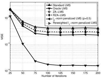
(a) $10$ dB SNR

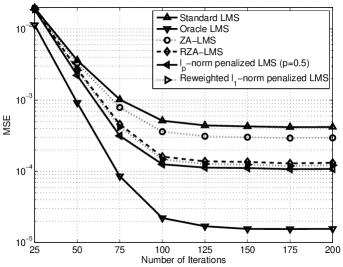
(b) $20$ dB SNR

Figure 1: Example 1, Case 1: MSE’s of different estimation algorithms vs number of iterations ($S=1$).

5.2 Simulation Example 2: Arbitrary Sparsity Basis

The ZA-LMS and RZA-LMS algorithms in the form derived in [7] are only applied to the case when the channel is sparse in the time domain. However, these algorithms as well as the $l_{p}$-pseudo-norm penalized LMS and reweighted $l_{1}$-norm penalized LMS algorithms can be modified to accommodate the case of an arbitrary sparsity basis. Consider the ZA-LMS algorithm in the case when the CIR is sparse in a sparsity domain denoted by $\boldsymbol{\Psi}$. The CIR representation in $\boldsymbol{\Psi}$, i.e., the vector ${\boldsymbol{w}}_{\Psi}=\boldsymbol{\Psi}\boldsymbol{w}$, is a sparse vector and it has a few nonzero entries. The corresponding update equation for the ZA-LMS algorithm is given by (53).

The update equation for the reweighted $l_{1}$-norm penalized LMS algorithm becomes

$$\boldsymbol{w}_{k+1}=\boldsymbol{w}_{k}+\mu e_{k}\boldsymbol{x}_{k}-\rho_{\rm r}\frac{\text{sgn}(\boldsymbol{\Psi}\boldsymbol{w}_{k})\boldsymbol{\Psi}}{\epsilon_{\rm r}+|\boldsymbol{\Psi}\boldsymbol{w}_{k-1}|}.$$ (56)

Finally, the modified update equation of the $l_{p}$-pseudo-norm penalized LMS algorithm can be derived as

$$\boldsymbol{w}_{k+1}=\boldsymbol{w}_{k}+\mu e_{k}\boldsymbol{x}_{k}-\rho_{\rm p}\frac{\left(\|\boldsymbol{\Psi}\boldsymbol{w}_{k}\|_{p}\right)^{1-p}\text{sgn}(\boldsymbol{\Psi}\boldsymbol{w}_{k})\boldsymbol{\Psi}}{\epsilon_{\rm p}+|\boldsymbol{\Psi}\boldsymbol{w}_{k}|^{(1-p)}}.$$ (57)

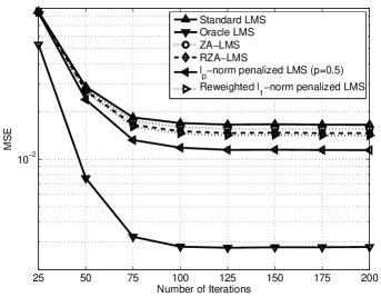
(a) $10$ dB SNR

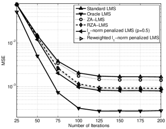
(b) $20$ dB SNR

Figure 2: Example 1, Case 2: MSE’s of different estimation algorithms vs number of iterations ($S=4$).

In this simulation example, a CIR of length $N=16$ with the sparsity level of $S=2$ is being estimated which is sparse in the discrete cosine transform (DCT) domain. The positions of nonzero taps in the DCT domain are chosen randomly. The value of the nonzero elements in the DCT domain are set to $1$ or $-1$ with the same probabilities each equal to half. The algorithms being compared here are the ZA-LMS, RZA-LMS, $l_{p}$-pseudo-norm penalized LMS, reweighted $l_{1}$-norm penalized LMS, and standard LMS algorithms. As in the first simulation scenario, two different SNR values of $10$ and $20$ dBs are tested. Parameter choices for the $10$ dB SNR case are as follows. For the $l_{p}$-pseudo-norm penalized LMS algorithm, $p=1/2$, $\epsilon_{\rm p}=0.05$, and $\rho_{\rm p}=2\times 10^{-4}$. Parameters of the reweighted $l_{1}$-norm penalized LMS algorithm are $\rho_{\rm r}=2\times 10^{-4}$ and $\epsilon_{\rm r}=0.05$. For the ZA-LMS and the RZA-LMS algorithms, the values are $\rho_{\rm ZA}=5\times 10^{-4}$, $\rho_{\rm RZA}=4\times 10^{-3}$, and $\epsilon_{\rm RZA}=25$. The step size $\mu$ is set to $0.05$. For the $20$ dB SNR case, $\rho_{\rm r}$, $\rho_{\rm p}$, and $\rho_{\rm RZA}$ are reduced by half.

The MSE curves in Fig. 3 are averaged over $10000$ simulation runs. The same conclusions as in Simulation Example 1 hold here as well. For the SNR of $10$ dB SNR, the $l_{p}$-pseudo-norm penalized LMS algorithm outperforms all the other algorithms followed by the reweighted $l_{1}$-norm penalized LMS algorithm, and then by the RZA-LMS and ZA-LMS algorithms. However, when the SNR is set to $20$ dB, the reweighted $l_{1}$-norm penalized LMS and RZA-LMS algorithms show a better performance than the $l_{p}$-pseudo-norm penalized LMS algorithm.

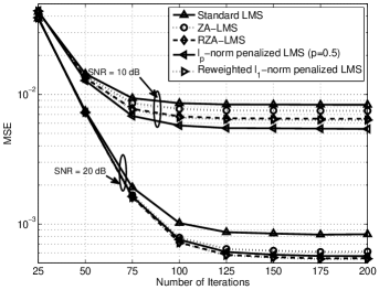
Figure 3: Example 2: MSEs of estimation algorithms vs number of iterations for a DCT sparse channel with $S=2$.

5.3 Simulation Example 3: Effect of Sparsity Level on the Performance of the Reweighted $l_{1}$-norm Penalized LMS Algorithm

In this example, we study the effect that the increasing sparsity level of CIR has on the performance of the reweighted $l_{1}$-norm penalized LMS algorithm. A CIR is assumed to be sparse in the time domain and it is of length $N=16$. The sparsity level varies from $2$ to $8$. The positions of the nonzero taps of the CIR are chosen randomly and the values of nonzero taps are set to $1$ or $-1$ with equal probability each equal to half. Parameters of the reweighted $l_{1}$-norm penalized LMS algorithm are $\rho_{\rm r}=2\times 10^{-4}$ and $\epsilon_{\rm r}=0.05$. The step size $\mu$ is set to $0.05$. Variance of the additive noise term $n_{k}$ is $\sigma^{2}_{\rm n}=0.01$. Excess MSE is used as a performance measure in this example. We have chosen a constant variance $\sigma^{2}_{\rm n}$ for the noise in order to make sure that the standard LMS algorithm has the same excess MSE regardless of the sparsity level of the channel. The excess MSE curves are averaged over $10000$ simulation runs. According to (5), the excess MSE can be derived as $\xi_{k}=\text{tr}\left\{\boldsymbol{R}E\big{[}\boldsymbol{v}_{k}\boldsymbol{v}^{T}_{k}\big{]}\right\}$. In this simulation example with $\boldsymbol{x}_{k}$ being an i.i.d. binary phase-shift keying (BPSK) sequence, the covariance matrix $\boldsymbol{R}$ becomes identity, and therefore, $\xi_{k}$ can be evaluated as $\text{tr}\left\{E\big{[}\boldsymbol{v}_{k}\boldsymbol{v}^{T}_{k}\big{]}\right\}$.

Fig. 4 shows the excess MSE versus the number of iterations for the standard LMS and reweighted $l_{1}$-norm penalized LMS algorithms when the CIR sparsity level is varied from $2$ to $8$. It can be seen that the standard LMS algorithm results in the same excess MSE regardless of the sparsity level of the CIR. However, the excess MSE of the reweighted $l_{1}$-norm penalized LMS algorithm increases with increasing sparsity level which is due to the fact that the value of $\alpha^{\prime}$ in equation (4.2) is decreasing. For example, $\alpha^{\prime}$ is equal to $2.7$, $2.3$, $2.0$, and $1.6$ for sparsity levels of 2, 4, 6, and 8, respectively, after $150$ iterations. It can be also seen that in all cases, the reweighted $l_{1}$-norm penalized LMS algorithm outperforms the standard LMS algorithm.

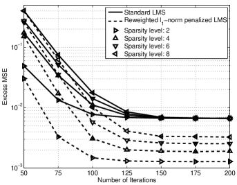
Figure 4: Example 3: Excess MSE versus number of iterations.

6 Conclusions

Sparse channel estimation problem has been considered in this paper and the reweighted $l_{1}$-norm penalized LMS algorithm has been introduced and analyzed. Quantitative analysis of the reweighted $l_{1}$-norm penalized LMS algorithm and the attainable excess MSE have been presented. The excess MSE result shows that the reweighted $l_{1}$-norm penalized LMS algorithm outperforms the standard LMS algorithm for the case of sparse CIR. The analysis has enabled us also to answer the question of what is the maximum sparsity level in the channel for which the reweighted $l_{1}$-norm penalized LMS algorithm is better than the standard LMS. Update equations of the reweighted $l_{1}$-norm penalized LMS, ZA-LMS, and the $l_{p}$-pseudo-norm penalized LMS algorithms have been generalized to the case of an arbitrary sparsity basis. Simulation results for the DCT sparse channel are given along with simulation results for the time sparse channel. The performance of the reweighted $l_{1}$-norm penalized LMS algorithm has been compared to that of the standard LMS, ZA-LMS, RZA-LMS algorithms, and our earlier proposed $l_{p}$-pseudo-norm penalized LMS algorithm through computer simulations. These results show that the reweighted $l_{1}$-norm penalized LMS algorithm outperforms the standard LMS, ZA-LMS, and RZA-LMS algorithms in all examples. It is also worth mentioning that variable step size is known to lead to better steady state error and therefore, better performance. Thus, as a further extention, the variable step size feature can be easily added to the proposed algorithm in the same way as it has been added to the RA-LMS in [29].

References

• [1] B. Widrow, and S. D. Stearns, Adaptive Signal Processing, Prentice Hall, 1985.
• [2] S. Haykin, Adaptive Filter Theory, Prentice Hall, 2002.
• [3] N. J. Bershad, J. M. Bermudez, and J. Y. Tourneret, “Stochastic analysis of the LMS algorithm for system identification with subspace inputs,” IEEE Trans. Signal Processing, vol. 56, no. 3, pp. 1018–1027, Mar. 2008.
• [4] H. I. K. Rao, and B. Farhang-Boroujeny, “Fast LMS/Newton algorithms for stereophonic acoustic echo cancellation,” IEEE Trans. Signal Processing, vol. 57, no. 8, pp. 2919–2930, Aug. 2009.
• [5] S. Coleri, M. Ergen, A. Puri, and A. Bahai, “Channel estimation techniques based on pilot arrangement in OFDM systems,” IEEE Trans. Broadcasting, vol. 48, no. 3, pp. 223–229, Sept. 2002.
• [6] O. Macchi, N. Bershad, and M. Mboup, “Steady-state superiority of LMS over LS for time-varying line enhancer in noisy environment,” IEE Proceedings Radar and Signal Processing, vol. 138, no. 4, pp. 354–360, Aug. 1991.
• [7] Y. Chen, Y. Gu, and A. O. Hero, “Sparse LMS for system identification,” in Proc. IEEE ICASSP, Taipei, Taiwan, Apr. 2009, pp. 3125–3128.
• [8] Y. Gu, J. Jin, and S. Mei, “$l_{0}$ norm constraint LMS algorithm for sparse system identification,” in IEEE Signal Processing Letters, vol. 16, no. 9, pp. 774–777, Sept. 2009.
• [9] K. Shi, and P. Shi, “Convergence analysis of sparse LMS algorithms with $l_{1}$-norm penalty based on white input signal,” ELSEVIER Signal Processing, vol. 90, no. 12, pp. 3289–3293, Dec. 2010.
• [10] G. Su, J. Jin, Y. Gu, and J. Wang, “Performance analysis of $l_{0}$ norm constraint least mean square algorithm,” IEEE Trans. Signal Processing, vol. 60, no. 9, pp. 2223–2235, May 2012.
• [11] K. Shi, and X. Ma, “Transform domain LMS for sparse system identification,” in Proc. IEEE ICASSP, Dallas, USA, Mar. 2010, pp. 3714–3717.
• [12] J. Yang, and G. E. Sobelman, “Sparse LMS with segment zero attractors for adaptive estimation of sparse signals,” in Proc. IEEE APCCAS, Kuala Lumpur, Malaysia, Dec. 2010, pp. 422–425.
• [13] Y. Murakami, M. Yamagishi, M. Yukawa, and I. Yamada, “A sparse adaptive filtering using time-varying soft-thresholding techniques,” in Proc. IEEE ICASSP, Dallas, USA, Mar. 2010, pp. 3734–3737.
• [14] O. Taheri and S. A. Vorobyov, “Decimated least mean squares for frequency sparse channel estimation,” in Proc. IEEE ICASSP, Kyoto, Japan, Mar. 25-30, 2012, pp. 3181-3184.
• [15] N. J. Bershad, and A. Bist, “Fast coupled adaptation for sparse impulse responses using a partial Haar transform,” IEEE Trans. Signal Processing, vol. 53, no. 3, pp. 966–976, Mar. 2005.
• [16] R. K. Martin, W. A. Sethares, R. C. Williamson, and C. R. Johnson, “Exploiting sparsity in adaptive filters,” IEEE Trans. Signal Processing, vol. 50, no. 8, pp. 1883–1894, Aug. 2002.
• [17] S. Chouvardas and K. Slavakis and Y. Kopsinis, and S. Theodoridis, “A sparsity promoting adaptive algorithm for distributed learning,” IEEE Trans. Signal Processing, vol. 60, no. 10, pp. 5412–5425, Oct. 2012.
• [18] P. Di Lorenzo, and A. H. Sayed, “Sparse distributed learning based on diffusion adaptation,” IEEE Trans. Signal Processing, vol. 61, no. 6, pp. 1419–1433, Mar. 2013.
• [19] D. Angelosante, J. A. Bazerque, and G. B. Giannakis, “Online adaptive estimation of sparse signals: where RLS meets the $l_{1}$-norm,” IEEE Trans. Signal Processing, vol. 58, pp. 3436–3447, July 2010.
• [20] B. Dumitrescu, A. Onose, P. Helin, and I. Tabus, “Greedy sparse RLS,” IEEE Trans. Signal Processing, vol. 60, no. 5, pp. 2194–2207, May 2012.
• [21] N. Vaswani, “Kalman filtered compressed sensing,” in Proc. IEEE ICIP, San Diego, USA, Oct. 2008, pp. 893–896.
• [22] E. J. Candes, and M. B. Wakin, “An introduction to compressive sampling,” IEEE Signal Processing Mag., vol. 25, no. 2, pp. 21–30, Mar. 2008.
• [23] D. Donoho, “Compressed sensing,” IEEE Trans. Inf. Theory, vol. 52, pp. 1289–1306, Apr. 2006.
• [24] O. Taheri, and S. A. Vorobyov, “Sparse channel estimation with $l_{p}$-norm and reweighted $l_{1}$-norm penalized least mean squares,” in Proc. IEEE ICASSP, Prague, Czech Republic, May 2011, pp. 2864–2867.
• [25] E. J. Candes, M. B. Wakin, and S. P. Boyd, “Enhancing sparsity by reweighted $l_{1}$ minimization,” Journal of Fourier Analysis and Applications, vol. 14, no. 5, pp. 877–905, Dec. 2008.
• [26] S. C. Douglas, and W. Pan, “Exact expectation analysis of the LMS adaptive filter,” IEEE Trans. Signal Processing, vol. 43, no. 12, pp. 2863–2871, Dec. 1995.
• [27] L. L. Horowitz, and K. D. Senne, “Performance advantage of complex LMS for controlling narrow-band adaptive arrays,” Proc. IEEE ICASSP, vol. 29, no. 3, pp. 722–736, June 1981.
• [28] B. Liu, and M. D. Sacchi, “Minimum weighted norm interpolation of seismic records,” Geophysics, vol. 69, no. 6, pp. 1560–1568, Nov.-Dec. 2004.
• [29] M. O. Bin Saeed and A. Zerguine, “A variable step size strategy for sparse system identification,” in Proc. 10th Intern. Multi-Conference on Systems, Signals, and Devices, Hammamet, Tunisia, Mar. 2013.