Predictive Control Algorithms: Stability despite Shortened Optimization Horizons

Abstract

: The stability analysis of model predictive control schemes without terminal constraints and/or costs has attracted considerable attention during the last years. We pursue a recently proposed approach which can be used to determine a suitable optimization horizon length for nonlinear control systems governed by ordinary differential equations. In this context, we firstly show how the essential growth assumption involved in this methodology can be derived and demonstrate this technique by means of a numerical example. Secondly, inspired by corresponding results, we develop an algorithm which allows to reduce the required optimization horizon length while maintaining asymptotic stability or a desired performance bound. Last, this basic algorithm is further elaborated in order to enhance its robustness properties.

1 Introduction

Within the last decades, model predictive control (MPC) has grown mature for both linear and nonlinear systems, see, e.g., Camacho and Bordons (2004) or Rawlings and Mayne (2009). Although analytically and numerically challenging, the method itself is attractive due to its simplicity: In a first step, a new measurement of the current system state is obtained which is thereafter used to compute an optimal control over a finite optimization horizon. In the third and last step, a portion of this control is applied to the process and the entire problem is shifted forward in time rendering the scheme to be iteratively applicable.

Stability of the MPC closed loop can be shown by imposing endpoint constraints, Lyapunov type terminal costs or terminal regions, cf. Keerthi and Gilbert (1988) and Chen and Allgöwer (1998). Here, we study MPC schemes without these ingredients for which stability and, in addition, bounds on the required horizon length can be deduced, both for linear and nonlinear systems, cf. Primbs and Nevistić (2000) and Tuna et al. (2006). We follow the recent approach from Reble and Allgöwer (2011) extending Grüne (2009); Grüne et al. (2010) to continuous time systems which not only guarantees stability but also reveals an estimate on the degree of suboptimality with respect to the optimal controller on an infinite horizon.

In this work, we show how the essential assumption needed to apply the methodology proposed in Reble and Allgöwer (2011) can be practically verified. Then, based on observations drawn from numerical computations, implementable MPC algorithms with variable control horizons are developed which allow for smaller optimization horizons while maintaining stability or a desired performance bound. To overcome the lack of robustness implied by prolonging the control horizon and, thus, staying in open loop for longer time intervals, conditions are presented which ensure that the control loop can be closed more often. Similar ideas were introduced in Pannek and Worthmann (2011) for a discrete time setting. Last, the computational effort is further reduced by introducing slack which allows to violate our main stability condition — a relaxed Lyapunov inequality — temporarily, cf. Giselsson (2010).

The paper is organized as follows: In Section 2 the problem formulation is given. In the ensuing Section 3, we summarize stability results from Reble and Allgöwer (2011) and propose a technique to verify the key assumption which is illustrated by an example. Thereafter, we present algorithms which allow for shortening the optimization horizon by using time varying control horizons. Before drawing conclusions, Section 5 contains results on how stability may be guaranteed by using weaker stability conditions.

2 Setup and Preliminaries

Let $\mathbb{N}$ and $\mathbb{R}$ denote the set of natural and real numbers respectively and $\|\cdot\|$ the Euclidean norm on $\mathbb{R}^{d}$, $d\in\mathbb{N}$. A continuous function $\eta:\mathbb{R}_{\geq 0}\rightarrow\mathbb{R}_{\geq 0}$ is called class $\mathcal{K}_{\infty}$-function if it satisfies $\eta(0)=0$, is strictly increasing and unbounded. A continuous function $\beta:\mathbb{R}_{\geq 0}\times\mathbb{R}_{\geq 0}\rightarrow\mathbb{R}_{\geq 0}$ is said to be of class $\mathcal{KL}$ if for each $r>0$ we have that $\lim_{t\rightarrow\infty}\beta(r,t)=0$ holds, and for each $t\geq 0$ the condition $\beta(\cdot,t)\in\mathcal{K}_{\infty}$ is satisfied.

Within this work we consider nonlinear time invariant control systems

$$\dot{x}(t)=f(x(t),u(t))$$ (1)

where $x(t)\in\mathbb{R}^{n}$ and $u(t)\in\mathbb{R}^{m}$ denote the state and control at time $t\geq 0$. Constraints can be included via suitable subsets $\mathbb{X}\subset\mathbb{R}^{n}$ and $\mathbb{U}\subset\mathbb{R}^{m}$ of the state and control space, respectively. We denote a state trajectory which emanates from the initial state $x_{0}$ and is subject to the control function $u:\mathbb{R}_{\geq 0}\rightarrow\mathbb{R}^{m}$ by $x_{u}(t)=x_{u}(t;x_{0})$. In the presence of constraints, a control function $u$ is called admissible for $x$ on the interval $[0,T)$ if the corresponding solution $x_{u}(\cdot;x)$ exists and satisfies

$$x_{u}(t;x)\in\mathbb{X},t\in[0,T],\quad\;\text{and}\;\quad u(t)\in\mathbb{U},t\in[0,T).$$ (2)

The set of these admissible control functions is denoted by $\mathcal{U}_{x}([0,T))$. For an infinite time interval, $u:\mathbb{R}_{\geq 0}\rightarrow\mathbb{R}^{m}$ is called admissible for $x$ if $u|_{[0,T)}\in\mathcal{U}_{x}([0,T))$ holds for each $T>0$ and the respective set is denoted by $\mathcal{U}_{x}([0,\infty))$.

For system (1) we assume an equilibrium $(x^{\star},u^{\star})\in\mathbb{X}\times\mathbb{U}$ to exist, i.e. $f(x^{\star},u^{\star})=0$ holds. Our goal is to design a feedback control law $\mu:\mathbb{R}^{n}\rightarrow\mathbb{R}^{m}$ such that the resulting closed loop is asymptotically stable with respect to $x^{\star}$, i.e. there exists $\beta\in\mathcal{KL}$ such that $\|x_{\mu}(t;x_{0})-x^{\star}\|\leq\beta(\|x_{0}-x^{\star}\|,t)$, $t\geq 0$, holds for all $x_{0}\in\mathbb{X}$ where $x_{\mu}(\cdot;x_{0})$ denotes the closed loop trajectory induced by $\mu$. The stabilization task is to be accomplished in an optimal fashion which is measured by a cost functional. To this end, we introduce the continuous running cost $\ell:\mathbb{R}^{n}\times\mathbb{R}^{m}\to\mathbb{R}_{\geq 0}$ satisfying

$$\ell(x^{\star},u^{\star})=0\quad\text{and}\quad\inf_{u\in\mathbb{U}}\ell(x,u)>0\ \forall\,x\neq x^{\star}.$$

Then, for a given state $x\in\mathbb{X}$, the cost of an admissible control $u\in\mathcal{U}_{x}([0,\infty))$ is

$$J_{\infty}(x,u):=\int_{0}^{\infty}\ell(x_{u}(t;x),u(t))\,dt.$$

The computation of a corresponding minimizer is, in general, computationally hard due to the curse of dimensionality, cf. Bardi and Capuzzo-Dolcetta (1997). Hence, we use model predictive control (MPC) to approximately solve this task. The central idea of MPC is to truncate the infinite horizon, i.e. to compute a minimizer $u^{\star}\in\mathcal{U}_{x}([0,T))$ of the cost functional

$$J_{T}(x,u):=\int_{0}^{T}\ell(x_{u}(t;x),u(t))\,dt,$$ (3)

which can be done efficiently using discretization methods and nonlinear optimization algorithms, see, e.g., Maciejowski (2002) or (Grüne and Pannek, 2011, Chapter 10). Furthermore, we define the corresponding optimal value function $V_{T}(x):=\inf_{u\in\mathcal{U}_{x}([0,T))}J_{T}(x,u)$, $T\in\mathbb{R}_{\geq 0}\cup\{\infty\}$.

To obtain an infinite horizon control, only the first portion of the computed minimizer is applied, i.e. we define the feedback law via

$$\mu_{T,\delta}(t;x):=u^{\star}(t),\quad t\in[0,\delta),$$ (4)

for the so called control horizon $\delta\in(0,T)$. Last, the optimal control problem is shifted forward in time which renders Algorithm 1 to be iteratively applicable.

Algorithm 1 MPC

Given: $T>\delta>0$

1. Measure the current state $\hat{x}$

2. Compute a minimizer $u^{\star}\in\mathcal{U}_{\hat{x}}([0,T))$ of (3) and define the MPC feedback law via (4)

3. Implement $\mu_{T,\delta}(t;\hat{x})|_{t\in[0,\delta)}$, shift the horizon forward in time by $\delta$ and goto (1)

The closed loop state trajectory emanating from the initial state $x_{0}$ subject to the MPC feedback law $\mu_{T,\delta}$ from Algorithm 1 is denoted by $x_{\mu_{T,\delta}}(\cdot;x_{0})$. Furthermore, $u_{\text{MPC}}^{\mu_{T,\delta}}:\mathbb{R}_{\geq 0}\rightarrow\mathbb{R}^{m}$ denotes the control function obtained by concatenating the applied pieces of control functions, i.e.

$$u_{\text{MPC}}^{\mu_{T,\delta}}(t;x_{0})=\mu_{T,\delta}(t-\lfloor t/\delta\rfloor\delta,x_{\mu_{T,\delta}}(\lfloor t/\delta\rfloor\delta;x_{0})).$$

The resulting MPC closed loop cost are given by

$$V_{\infty}^{\mu_{T,\delta}}(x):=\int_{0}^{\infty}\ell(x_{\mu_{T,\delta}}(t;x),u_{\text{MPC}}^{\mu_{T,\delta}}(t))\,dt.$$

Note that we tacitly assume that Problem (3) is solvable for all $x_{0}\in\mathbb{X}$ and the minimum is attained in each step of Algorithm 1. For a detailed discussion of feasibility issues we refer to (Grüne and Pannek, 2011, Chapter 8).

3 Stability and Performance Bounds

Due to the truncation of the infinite horizon, stability and optimality properties of the optimal control may be lost. Yet, stability can be shown if the optimization horizon is sufficiently long, cf. Alamir and Bornard (1995); Jadbabaie and Hauser (2005). Additionally, an optimization horizon length $T$ can be determined for which both asymptotic stability as well as a performance bound on the MPC closed loop in comparison to the infinite horizon control law hold.

Theorem 3.1

Suppose a control horizon $\delta>0$ and a monotone bounded function $B:\mathbb{R}_{\geq 0}\to\mathbb{R}_{\geq 0}$ satisfying

$$V_{t}(x)\leq B(t)\inf_{u\in\mathbb{U}}\ell(x,u)=:B(t)\ell^{\star}(x),\quad t\geq 0,$$ (5)

for all $x\in\mathbb{X}$ to be given. If $T>\delta$ is chosen such that $\alpha_{T,\delta}>0$ holds for

$$\alpha_{T,\delta}:=1-\frac{e^{-\int_{\delta}^{T}B(t)^{-1}dt}e^{-\int_{T-\delta}^{T}B(t)^{-1}dt}}{\left[1-e^{-\int_{\delta}^{T}B(t)^{-1}dt}\right]\left[1-e^{-\int_{T-\delta}^{T}B(t)^{-1}dt}\right]},$$ (6)

then the relaxed Lyapunov inequality

$$V_{T}(x)-V_{T}(x_{\mu_{T,\delta}}(\delta;x))\geq\alpha_{T,\delta}\int_{0}^{\delta}\ell(x_{\mu_{T,\delta}}(t;x),\mu_{T,\delta}(t;x))dt$$ (7)

as well as the performance estimate

$$V_{\infty}^{\mu_{T,\delta}}(x)\leq\alpha_{T,\delta}^{-1}V_{\infty}(x)$$ (8)

are satisfied for all $x\in\mathbb{X}$. If, additionally, there exist $\mathcal{K}_{\infty}$ functions $\underline{\eta}$, $\overline{\eta}$ such that $\underline{\eta}(x)\leq\ell^{\star}(x)\leq\overline{\eta}(x)$ hold for all $x\in\mathbb{X}$, then the MPC closed loop is asymptotically stable for horizon length $T$.

A detailed proof of Theorem 3.1 is given in Reble and Allgöwer (2011). We point out that for a given control horizon $\delta>0$ and a desired performance specification $\overline{\alpha}\in[0,1)$ on the MPC closed loop, there always exists an optimization horizon $T>\delta$ such that $\alpha_{T,\delta}>\overline{\alpha}$ is satisfied, cf. Worthmann (2012). Interpreting (8) exemplarily, the choice $\overline{\alpha}=0$ corresponds to asymptotic stability of the MPC closed loop whereas $\overline{\alpha}=0.5$ limits the cost of the MPC control to double the cost of the infinite horizon control.

The crucial assumption which has to be verified in order to apply Theorem 3.1 is the growth condition (5). Here, we demonstrate this by means of the following example:

Example 3.2

Consider the system dynamics of a synchronous generator given by

$$\dot{x}_{1}(t) =x_{2}(t)$$

$$\dot{x}_{2}(t) =-b_{1}x_{3}(t)\sin(x_{1}(t))-b_{2}x_{2}(t)+P$$

$$\dot{x}_{3}(t) =b_{3}\cos(x_{1}(t))-b_{4}x_{3}(t)+E+u(t)$$

with constants $b_{1}=34.29$, $b_{2}=0.0$, $b_{3}=0.149$, $b_{4}=0.3341$, $P=28.22$ and $E=0.2405$, cf. Galaz et al. (2003). The equilibrium we wish to stabilize is located at $x^{\star}=(1.124603730,0,0.9122974248)^{\top}$ and the running costs are defined as

$$\ell(x(t),u(t))=\|x(t)-x^{\star}\|_{2}^{2}+\lambda\|u(t)\|_{2}^{2}$$

where the parameter $\lambda=0.01$ is used to penalize the taken control effort. Due to physical considerations $x_{1}$ and $x_{3}$ are restricted to the interval $[0,\pi/2]$ and $\mathbb{R}_{\geq 0}$ respectively.

For Example 3.2, we want to determine an optimization horizon length $T$ such that asymptotic stability of the resulting MPC closed loop is guaranteed, i.e. $\overline{\alpha}=0$.

To achieve this goal, the following methodology can be applied to compute a function $B(\cdot)$ such that (5) holds:

1. For each state $x\in\mathbb{X}$ derive a monotone function $B_{x}:\mathbb{R}_{\geq 0}\rightarrow\mathbb{R}_{\geq 0}$ satisfying

   $$V_{t}(x)\leq B_{x}(t)\ell^{\star}(x)\qquad\forall\,t\geq 0.$$ (9)

2. Then, $B(t)$ is defined pointwise as $\sup_{x\in\mathbb{X}}B_{x}(t)$.

To accomplish Step (1) we exploit the fact that optimality of this bound is not needed. Hence, for each $t\in\mathbb{N}\cdot\Delta$ for some $\Delta>0$ we solve

$$\min_{u\in\mathcal{U}_{x}([0,t))}J_{t}(x,u)$$

over the class of sampled data systems with zero order hold and sampling period $\Delta$, i.e. control functions satisfying $u(t)=\text{\em constant}$ for $t\in[(n-1)\Delta,n\Delta)$, $n\in\mathbb{N}$. This yields monotone bounds $B_{x}(t)$, $t\in\Delta\mathbb{N}$, satisfying (9) by dividing by $\ell^{\star}(x)=\|x-x^{\star}\|$. Then, Step (2) is carried out in order to compute $B(t)$. Since neither terminal constraints nor costs were imposed, $V_{t}(x)$ is monotonically increasing in $t$ which implies $V_{t}(x)\leq V_{n\Delta}(x)\leq B(n\Delta)\ell^{\star}(x)$, $t\in((n-1)\Delta,n\Delta]$. Note that $B$ is only computed on a “sufficiently” large interval $[0,n^{\star}\Delta]$, $n^{\star}\in\mathbb{N}$, such that a desired performance estimate can be concluded by Theorem 3.1.

While the proposed procedure allows to verify Step (1) rigorously, we carry out Step (2) only approximately. The reason is twofold: Firstly, throughout this paper we assume feasibility for the set $\mathbb{X}$, i.e. $\mathbb{X}$ is control invariant, cf. Blanchini (1999) for a definition of control invariance. Hence, a suitable subset has to be computed a priori if this assumption is violated, see (Grüne and Pannek, 2011, Chapter 8). For Example 3.2, numerical computations show that an appropriately chosen level set $\mathcal{L}$ of the value function $V_{0.6}$ is control invariant. Secondly, this set has to be discretized. To this end, a grid of initial values $\mathcal{G}$ with discretization stepsize $\Delta_{x_{i}}$ within each direction $i\in\{1,\ldots,n\}$ is used. Then, $B(t)$ is approximately determined for the set $\mathcal{L}$ by taking the supremum with respect to all states contained in the intersection $\overline{X}:=\mathcal{L}\cap\mathcal{G}$.

In conclusion, the proposed approach allows to rigorously ensure the relaxed Lyapunov inequality except for the state space discretization assuming that a control invariant set is given.

Example 3.3

Regarding Example 3.2, let $\Delta=0.0125$ and the control horizon $\delta=0.05$ be given. Additionally, we define $\mathcal{G}:=[x^{\star}_{1}-a_{1},x^{\star}_{1}+a_{1}]\times[x^{\star}_{2}-a_{2},x^{\star}_{2}+a_{2}]\times[x^{\star}_{3}-a_{3},x^{\star}_{3}+a_{3}]$ with $a_{1}=0.4$, $a_{2}=0.5$, $a_{3}=0.9$ and discretization stepsize $\Delta_{x_{i}}:=0.02$, $i\in\{1,2,3\}$, and focus on the level set $\mathcal{L}:=\{x\mid V_{0.6}(x)\leq 0.0081\}$ whose convex hull satisfies all physical constraints, see Figure 1 for an illustration of $\overline{X}:=\mathcal{L}\cap\mathcal{G}$.

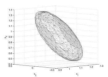
Figure 1: Illustration of the set $\overline{X}:=\mathcal{L}\cap\mathcal{G}$.

Then, Formula (6) enables us to determine an optimization horizon $T$ such that the relaxed Lyapunov inequality (7) holds with $\alpha_{T,\delta}>\overline{\alpha}=0$. For the computed function $B$ this methodology yields asymptotic stability of the MPC closed loop for optimization horizon $T=2.6$.

Remark 3.4

Note that the presented method verifies condition (5) for control functions $u\in\mathcal{L}^{\infty}([0,T),\mathbb{R}^{m})$, and allows to conclude asymptotic stability of the closed loop via Theorem 3.1, cf. (Worthmann et al., 2012, Remark 2.7).

4 Impact of the Control Horizon

In Section 3 we showed how to ensure asymptotic stability for the proposed MPC scheme for a given $\delta$. In this section, we investigate the impact of $\delta$ on the required optimization horizon length $T$.

Considering Example 3.2, we compute $\alpha_{T,\Delta}$, $\Delta=0.05$, and $\alpha_{T,T/2}$ for $T=n\Delta$, $n\in\{2,3,\ldots,60\}$, cf. Figure 2a. Here, $\alpha_{T,\Delta}>0$ holds for $T\geq 2.6=52\Delta$ whereas this stability criterion holds for significantly shorter optimization horizons if the control horizon is chosen equal to $T/2$, that is $\alpha_{T,T/2}>0$ for $T\geq 1.25=25\Delta$. Hence, enlarging the control horizon seems to induce an improved performance index $\alpha_{T,\delta}$.

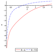
a) b)

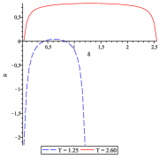
Figure 2: a) Development of $\alpha_{T,\delta}$ for varying $T$ and different choices of $\delta$. b) Development of $\alpha_{T,\delta}$ depending on the control horizon $\delta$.

This numerical result motivates to investigate the influence of $\delta$ on $\alpha_{T,\delta}$. To this end, we fix the optimization horizon $T$ and compute $\alpha_{T,n\Delta}$ for $n\in\{1,2,\ldots,T/\Delta-1\}$, cf. Figure 2b, which leads to the following observations: Firstly, a symmetry property seems to hold, i.e. $\alpha_{T,\delta}=\alpha_{T,T-\delta}$. Secondly, the performance estimates appear to increase up to the symmetry axis $T/2$. Both properties have been shown for systems which are exponentially controllable in terms of their stage costs, i.e. $\widetilde{B}(t)=C\int_{0}^{t}e^{-\mu s}\,ds$ for an overshoot constant $C\geq 1$ and a decay rate $\mu>0$, cf. Grüne et al. (2012). Using the computed function $B$ instead of exponential decay we obtain $\widetilde{B}(t)\geq B(t)$ and therefore better horizon estimates as shown in Worthmann (2011) for a discrete time setting. Despite the more general setting, symmetry still follows directly from Formula (6).

Corollary 4.1

The performance estimate $\alpha_{T,\delta}$ given by Formula (6) satisfies $\alpha_{T,\delta}=\alpha_{T,T-\delta}$ for $\delta\in(0,T)$, i.e. $\alpha_{T,\delta}$ is symmetric with symmetry axis $\delta=T/2$.

Unlike symmetry, we conjecture that there exists a counterexample negating monotonicity even if $B$ satisfies the additional condition (Reble and Allgöwer, 2011, Inequality (21)) which is, however, violated in Example 3.2. For such an example (5) holds but $\alpha_{T,\delta}$ is not monotone on $(0,T/2]$, cf. Grüne et al. (2010) for a counterexample in the discrete time setting.

Yet, for Example 3.2 numerical results indicate that the monotonicity property holds and allows to conclude asymptotic stability of the MPC closed loop for significantly shorter optimization horizons.

Example 4.2

Again consider Example 3.2. If we impose the horizon $T=1.25$, then from Figure 2b we observe that stability of the closed loop can only be guaranteed if $\delta\in[0.45,0.8]$. If the horizon length is increased to $T=2.60$, Figure 2a shows that for any chosen $\delta\in[0.05,2.55]$ stability can be concluded.

In the context of arbitrary monotone and bounded functions $B:\mathbb{R}_{\geq 0}\rightarrow\mathbb{R}_{\geq 0}$ another interesting fact arises if we consider arbitrarily small $\delta$:

Theorem 4.3

For any optimization horizon $T>0$ we have that $\alpha_{T,\delta}$ goes to $-\infty$ for $\delta\rightarrow 0$. In particular, our stability condition $\alpha_{T,\delta}\geq 0$ cannot be maintained for arbitrarily small control horizon $\delta$.

Proof: Follows directly from Formula (6).∎

Note that this assertion was solely shown for an exponentially controllable setting both for discrete and continuous time systems, cf. (Reble and Allgöwer, 2011, Section 4) and (Worthmann, 2011, Section 5.1). Hence, the key contribution is the observation that this conclusion can also be drawn without the restriction to this particular class of systems.

Motivated by Example 4.2 and Theorem 4.3, we propose an algorithm to obtain a control horizon length $\delta$ such that $\alpha_{T,\delta}$ exceeds a predefined suboptimality bound $\overline{\alpha}$. To this end, we introduce a partition $(\tau_{k})_{k\in\{0,\ldots,n\}}$, $n\in\mathbb{N}_{>1}$, of $[0,T]$ with $0=\tau_{0}<\tau_{1}<\ldots<\tau_{n}=T$. Such a setting naturally arises in the context of digital control for sampled data systems with zero order hold. Yet, we like to note that Algorithm 2 is not limited to the digital control case. Additionally, we like to stress that monotonicity of $\alpha_{T,\delta}$ in $\delta$ is the center of this algorithm.

Algorithm 2 MPC with increased control horizon

Given: $T>0$, $(\tau_{k})_{k\in\{0,\ldots,n\}}$ with $n\in\mathbb{N}_{>1}$ and $\overline{\alpha}\in[0,1)$

1. Measure the current state $\hat{x}$

2. Set $k:=0$ and compute a minimizer $u^{\star}\in\mathcal{U}_{\hat{x}}([0,T))$ of (3) and $V_{T}(\hat{x})=J_{T}(\hat{x},u^{\star})$.
   Do

   1. If $(k+1)=n$: Set $\delta$ according to exit strategy and goto (3)

   2. Set $k:=k+1$, $\delta:=\tau_{k}$ and compute $V_{T}(x_{u^{\star}}(\delta;\hat{x}))$

   3. Compute $\alpha_{T,\delta}$, i.e.

      $$\alpha_{T,\delta}:=\frac{V_{T}(\hat{x})-V_{T}(x_{u^{\star}}(\delta;\hat{x}))}{\int_{0}^{\delta}\ell(x_{u^{\star}}(t;\hat{x}),u^{\star}(t))\,dt}$$ (10)

   while $\alpha_{T,\delta}\leq\overline{\alpha}$

3. Implement $\mu_{T,\delta}(t;\hat{x})|_{t\in[0,\delta)}$, shift the horizon forward in time by $\delta$ and goto (1)

Algorithm 2 combines two aspects: the improved performance estimates obtained for larger control horizons $\delta$, and the inherent robustness resulting from using a feedback control law which benefits from updating the control law as often as possible. In order to illustrate this claim let us consider the numerical Example 3.2 again. From Figure 2b we observed that asymptotic stability of the MPC closed loop can be shown for $T\geq 1.25$. Indeed, Algorithm 2 only uses $\delta=\Delta=0.05$ in each step independent of the chosen initial condition. Hence, MPC with constant control horizon $\delta=0.05$ is performed safeguarded by our theoretically obtained estimates. Consequently, no exit strategy is needed since Step (2a) is excluded.

We compute $\alpha_{T,\delta}$ by Equation (10) for all $x\in\overline{X}$ in order to test out the limits of Algorithm 2. Here, $T=0.45$ is the smallest optimization horizon such that $\alpha_{T,\Delta}=\alpha_{T,\Delta}(x)>0$ is satisfied for all $x\in\overline{X}$. However, using Algorithm 2 allows to ensure this conditions for $T=0.25$ for varying control horizon $\delta\in\{\Delta,2\Delta,3\Delta,4\Delta\}$. Figure 3 shows the sets of states $x\in\overline{X}$ for which $\alpha_{T,\delta}$ computed by (10) is less than zero for the cases $\delta=\Delta$ and $\delta\in\{\Delta,2\Delta\}$. Again, we see that if we allow for larger control horizons $\delta$, then the performance bound $\alpha_{T,\delta}$ increases, i.e. the set of state vectors for which stability cannot be guaranteed shrinks. Hence, for the considered Example 3.2 Algorithm 2 allows to drastically reduce the horizon $T$ while maintaining asymptotic stability of the closed loop.

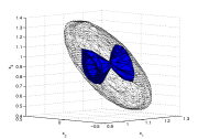
a) b)

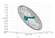
Figure 3: Set of initial values $x$ for which stability cannot be guaranteed for $T=0.45$, $\Delta=0.05$ with (a) $\delta=\Delta$ and (b) $\delta\in\{\Delta,2\Delta\}$.

The downside of considering potentially large control horizons $\delta$ is the possible lack of robustness in case of disturbances. Utilizing the introduced partition $(\tau_{k})_{k\in\{0,\ldots,n\}}$, we can perform an update of the feedback law at time $\tau_{j}\in\{0,\ldots,n\}$ via

$$\mu_{T,\delta}(t;x):=u^{\star}(t-\tau_{j};x_{\mu_{T,\delta}}(\tau_{j};x)),\quad t\geq\tau_{j},$$ (11)

where we extended the notation of the open loop optimal control to $u^{\star}(t;x)$ to indicate which initial state is considered. Such an update can be applied whenever the following Lyapunov type update condition holds, see also Pannek and Worthmann (2011) for the discrete time setting.

Proposition 4.4

Let $\overline{\alpha}\in[0,1)$, $T>0$ and a partition $(\tau_{k})_{k\in\{0,\ldots,n\}}$, $n\in\mathbb{N}$, of $[0,T]$ with $0=\tau_{0}<\tau_{1}<\ldots<\tau_{n}=T$ be given. For $\delta=\tau_{k}$ suppose (7) holds with $\alpha_{T,\delta}>\overline{\alpha}$ for some $x\in\mathbb{X}$. Let $u^{\star}(\cdot;x_{\mu_{T,\delta}}(\tau_{j};x))$ be a minimizer of (3) for some $j\in\{1,\ldots,k-1\}$. If additionally

$$V_{T}(x_{u^{\star}}(\tau_{k}-\tau_{j};x_{\mu_{T,\delta}}(\tau_{j};x)))-V_{T-\tau_{j}}(x_{\mu_{T,\delta}}(\tau_{j};x))$$

$$<(1-\overline{\alpha})\int_{0}^{\tau_{j}}\ell(x_{\mu_{T,\delta}}(t;x),\mu_{T,\delta}(t;x))dt$$ (12)

$$-\overline{\alpha}\int_{0}^{\tau_{k}-\tau_{j}}\ell(x_{u^{\star}}(t;x_{\mu_{T,\delta}}(\tau_{j};x)),u^{\star}(t;x_{\mu_{T,\delta}}(\tau_{j};x)))dt$$

holds, then the respective MPC feedback law $\mu_{T,\delta}(\cdot;x)$ can be modified by (11) and the lower bound $\overline{\alpha}$ on the degree of suboptimality is locally maintained.

We like to stress that if the stabilizing partition index $k$ is known, then Proposition 4.4 allows for iterative updates of the feedback until this index is reached. Hence, only Step (3) of Algorithm 2 needs to be adapted, see Algorithm 3 for a possible implementation.

Algorithm 3 MPC with intermediate update

1. For $n=0,\ldots k-1$ do

   1. Implement $\mu_{T,\delta}(t;\hat{x})|_{t\in[\tau_{n},\tau_{n+1})}$

   2. Compute $u^{\star}(\cdot;x_{\mu_{T,\delta}}(\tau_{n+1};\hat{x}))$

   3. If (12) holds: Update $\mu_{T,\delta}(\cdot;\hat{x})$ via (11)

   Shift the horizon forward in time by $\delta$ and goto (1)

5 Aggregated Performance

Usually, the relaxed Lyapunov inequality (7) is tight for only a few points in the state space. Hence, if a closed loop trajectory $x_{\mu_{T,\delta}}(\cdot;x)$ visits a point for which (7) is not an equality, then we can compute the occuring slack along the closed loop via

$$s(t,x):= V_{T}(x)-V_{T}(x_{\mu_{T,\delta}}(t;x))$$

$$-\overline{\alpha}\int_{0}^{t}\ell(x_{\mu_{T,\delta}}(s;x),u_{\text{MPC}}^{\mu_{T,\delta}}(s))\,ds.$$ (13)

This slack can be used to weaken the requirement (7) by considering the closed loop instead of the open loop solution. For simplicity of exposition, we formulate the following result using constant $\delta$, yet the conclusion also holds in the context of time varying control horizons as in Algorithm 2.

Theorem 5.1

Consider an admissible feedback law $u_{\text{MPC}}^{\mu_{T,\delta}}$, an initial value $x_{0}\in\mathbb{X}$ and $\overline{\alpha}\in(0,1)$ to be given. Furthermore, suppose there exist ${\mathcal{K}}_{\infty}$ functions $\underline{\eta}$, $\overline{\eta}$ such that $\ell^{\star}(x)\geq\underline{\eta}(\|x-x^{\star}\|)$ and $V_{T}(x)\leq\overline{\eta}(\|x-x^{\star}\|)$ hold for all $x\in\mathbb{X}$. If additionally $s(t,x)$ from (13) converges for $t$ tending to infinity, then the MPC closed loop trajectory with initial value $x_{0}$ behaves like an asymptotically stable solution. Furthermore, the following performance estimate holds

$$V_{\infty}^{\mu_{T,\delta}}(x_{0})\leq\frac{1-\lim_{t\rightarrow\infty}s(t,x_{0})/V_{T}(x_{0})}{\overline{\alpha}}V_{\infty}(x_{0}).$$ (14)

Proof: Let the limit of $s(t,x_{0})$ for $t\rightarrow\infty$ be denoted by $\theta$. Then, for given $\varepsilon>0$, there exists a time instant $t^{\star}$ such that $\|s(t,x_{0})-\theta\|\leq\varepsilon$ holds for all $t\geq t^{\star}$. As a consequence, we obtain

$$s(t,x_{0})= s(t^{\star},x_{0})-V_{T}(x_{\mu_{T,\delta}}(t;x_{0}))+V_{T}(x_{\mu_{T,\delta}}(t^{\star};x_{0}))$$

$$-\overline{\alpha}\int_{t^{\star}}^{t}\ell(x_{\mu_{T,\delta}}(s;x_{0}),u_{\text{MPC}}^{\mu_{T,\delta}}(s))\,ds\geq\theta-\varepsilon.$$

Since $V_{T}(x_{\mu_{T,\delta}}(t^{\star};x_{0}))\leq\overline{\eta}(\|x_{\mu_{T,\delta}}(t^{\star};x_{0})-x^{\star}\|)$ as well as $V_{T}(x_{\mu_{T,\delta}}(t;x_{0}))\geq 0$ hold, this inequality implies

$$2\varepsilon+\overline{\eta}(\|x_{\mu_{T,\delta}}(t^{\star};x_{0})-x^{\star}\|)$$

$$\geq s(t^{\star},x_{0})-\theta+\varepsilon+V_{T}(x_{\mu_{T,\delta}}(t^{\star};x_{0}))-V_{T}(x_{\mu_{T,\delta}}(t;x_{0}))$$

$$\geq \overline{\alpha}\int_{t^{\star}}^{t}\ell(x_{\mu_{T,\delta}}(s;x_{0}),u_{\text{MPC}}^{\mu_{T,\delta}}(s))\,ds.$$

Hence, boundedness of the integral on the right hand side can be concluded. Now, due to positivity and continuity of $\ell$ we have $\lim_{t\rightarrow\infty}\ell(x_{\mu_{T,\delta}}(t;x_{0}),u_{\text{MPC}}^{\mu_{T,\delta}}(t))=0$. In turn, the latter ensures $\underline{\eta}(\|x_{\mu_{T,\delta}}(t;x_{0})-x^{\star}\|)\rightarrow 0$ and, thus, $x_{\mu_{T,\delta}}(t;x_{0})\rightarrow x^{\star}$ for $t$ approaching infinity. Inequality (14) is shown by using

$$\lim_{t\rightarrow\infty}V_{T}(x_{\mu_{T,\delta}}(t;x))\leq\lim_{t\rightarrow\infty}\overline{\eta}(\|x_{\mu_{T,\delta}}(t;x)-x^{\star}\|)=0$$

in combination with (13) to obtain

$$\overline{\alpha}V_{\infty}^{\mu_{T,\delta}}(x) = \lim_{t\rightarrow\infty}\overline{\alpha}\int_{0}^{t}\ell(x_{\mu_{T,\delta}}(s;x),u_{\text{MPC}}^{\mu_{T,\delta}}(s))\,ds$$

$$= V_{T}(x)-\lim_{t\rightarrow\infty}s(t,x).$$

Then, since $V_{T}(x)\leq V_{\infty}(x)$, the assertion follows.∎

Note that within Theorem 5.1 we did not assume semipositivity but convergence of $s(t,x)$ to conclude stability. Here, we like to stress that $\lim_{t\rightarrow\infty}s(t,x)\geq 0$ implies a suboptimality index $\alpha_{T,\delta}\geq\overline{\alpha}$. Clearly, both the stability and performance result shown in Theorem 5.1 can be extended to assertions for all $x\in\mathbb{X}$ if $s(t,x)$ converges for every $x\in\mathbb{X}$ or a uniform lower bound can be found, i.e. $\inf_{x\in\mathbb{X}}\lim_{t\rightarrow\infty}s(t,x)=\theta>-\infty$.

Apart from its theoretical impact, $s(t,x)$ is also meaningful at runtime of the MPC algorithm. For instance, the condition $s(t,x)\geq 0$ can be checked at each time instant $t=n\delta$, $n\in\mathbb{N}$, instead of $\alpha_{T,\delta}>\overline{\alpha}$, cf. (10). This is particularly useful since accumulated slack can be used in order to compensate local violations of $\alpha_{T,\delta}\geq\overline{\alpha}$, i.e. weakening the stability condition (10), as long as the overall performance is still satisfactory.

If $s(t,x)<0$ occurs within the MPC algorithm, the slack can also be used to form an exit strategy. To this end, we denote the performance of the MPC closed loop until time $t$ by

$$\alpha(t):=\frac{V_{T}(x)-V_{T}(x_{\mu_{T,\delta}}(t;x))}{\int_{0}^{t}\ell(x_{\mu_{T,\delta}}(s;x),u_{\text{MPC}}^{\mu_{T,\delta}}(s))\,ds}.$$ (15)

Now, if $s(t,x)<0$ but $\alpha(t)>0$, then stability is still maintained, yet the current performance index is worse than the desired bound $\overline{\alpha}$.

Example 5.2

Again we consider Example 3.2 and analyze the MPC closed loop for $\mu_{T,\delta}$ with $T=0.25$ and $\delta=\Delta=0.05$. If we choose the initial value $x_{0}=(1.03960373,-0.085,0.9122974248)^{\top}$, then we observe from Figure 4 that the local estimate $\alpha_{T,\delta}$ drops below zero for $t=\delta$, i.e. stability cannot be guaranteed for $\delta=\Delta$. Yet, computing $\alpha(t)$ according to (15) shows that the relaxed Lyapunov inequality is satisfied after two steps of the MPC algorithm. Hence, using the slack information incorporated in $\alpha(t)$ allows to conclude asymptotic stability.

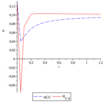
Figure 4: Development of $\alpha_{T,\delta}$ and $\alpha(t)$ for $T=0.25$ and $\delta=0.05$ along a specific closed loop solution.

6 Conclusions and Outlook

We have shown a methodology to verify the assumptions introduced in Reble and Allgöwer (2011) under which stability of the MPC closed loop without terminal constraints can be guaranteed. Additionally we presented an algorithmic approach for varying control horizons which allows to reduce the optimization horizon length. Last, we provided robustification methods via update and slack based rules.

This work was supported by the DFG priority research program 1305 “Control Theory of Digitally Networked Dynamical Systems”, grant. no. Gr1569/12-1, and by the German Federal Ministry of Education and Research (BMBF) project “SNiMoRed”, grant no. 03MS633G.

References

- Alamir and Bornard (1995) M. Alamir and G. Bornard. Stability of a truncated infinite constrained receding horizon scheme: the general discrete nonlinear case. Automatica, 31(9):1353–1356, 1995.
- Bardi and Capuzzo-Dolcetta (1997) M. Bardi and I. Capuzzo-Dolcetta. Optimal control and viscosity solutions of Hamilton-Jacobi-Bellman equations. Birkhäuser, 1997.
- Blanchini (1999) F. Blanchini. Set Invariance in Control. Automatica, 35:1747–1767, 1999.
- Camacho and Bordons (2004) E. F. Camacho and C. Bordons. Model Predictive Control. Springer, 2004.
- Chen and Allgöwer (1998) H. Chen and F. Allgöwer. A quasi-infinite horizon nonlinear model predictive control scheme with guaranteed stability. Automatica, 34(10):1205–1218, 1998.
- Galaz et al. (2003) M. Galaz, R. Ortega, A. S. Bazanella, and A. M. Stankovic. An energy-shaping approach to the design of excitation control of synchronous generators. Automatica, 39(1):111–119, 2003.
- Giselsson (2010) P. Giselsson. Adaptive Nonlinear Model Predictive Control with Suboptimality and Stability Guarantees. In Proceedings of the 49th Conference on Decision and Control, Atlanta, GA, USA, pages 3644–3649, 2010.
- Grüne (2009) L. Grüne. Analysis and design of unconstrained nonlinear MPC schemes for finite and infinite dimensional systems. SIAM Journal on Control and Optimization, 48:1206–1228, 2009.
- Grüne and Pannek (2011) L. Grüne and J. Pannek. Nonlinear Model Predictive Control: Theory and Algorithms. Springer, 2011.
- Grüne et al. (2010) L. Grüne, J. Pannek, M. Seehafer, and K. Worthmann. Analysis of unconstrained nonlinear MPC schemes with varying control horizon. SIAM Journal on Control and Optimization, 48(8):4938–4962, 2010.
- Grüne et al. (2012) L. Grüne, J. Pannek, and K. Worthmann. Ensuring Stability in Networked Systems with Nonlinear MPC for Continuous Time Systems. In Proceedings of the 51st Converence on Decision and Control, Maui, Hawaii, USA, 2012. To appear.
- Jadbabaie and Hauser (2005) A. Jadbabaie and J. Hauser. On the stability of receding horizon control with a general terminal cost. IEEE Trans. Automat. Control, 50(5):674–678, 2005. ISSN 0018-9286.
- Keerthi and Gilbert (1988) S. S. Keerthi and E. G. Gilbert. Optimal infinite horizon feedback laws for a general class of constrained discrete-time systems: stability and moving horizon approximations. Journal of Optimization Theory and Applications, 57:265–293, 1988.
- Maciejowski (2002) J. M. Maciejowski. Predictive Control with Constraints. Prentice-Hall, Harlow, England, 2002.
- Pannek and Worthmann (2011) J. Pannek and K. Worthmann. MPC Algorithms with Stability and Performance Guarantees. http://arxiv.org/pdf/1109.6153.pdf, 2011.
- Primbs and Nevistić (2000) J.A. Primbs and V. Nevistić. Feasibility and stability of constrained finite receding horizon control. Automatica, 36:965–971, 2000.
- Rawlings and Mayne (2009) J. B. Rawlings and D. Q. Mayne. Model Predictive Control: Theory and Design. Nob Hill Publishing, 2009.
- Reble and Allgöwer (2011) M. Reble and F. Allgöwer. Unconstrained Model Predictive Control and Suboptimality Estimates for Nonlinear Continuous-Time Systems. Automatica, 2011. Accepted.
- Tuna et al. (2006) S.E. Tuna, M.J. Messina, and A.R. Teel. Shorter horizons for model predictive control. In Proceedings of the 2006 American Control Conference, Minneapolis, Minnesota, USA, 2006.
- Worthmann (2011) K. Worthmann. Stability Analysis of Unconstrained Receding Horizon Control Schemes. PhD thesis, University of Bayreuth, 2011.
- Worthmann (2012) K. Worthmann. Estimates on the Required Prediction Horizon in MPC: A Numerical Case Study. In Proceedings of the Conference on Nonlinear Model Predicitve Control, Nordwijkerhout, the Netherlands, 2012. To appear.
- Worthmann et al. (2012) K. Worthmann, M. Reble, L. Grüne, and F. Allgöwer. The role of sampling for stability and performance in unconstrained model predictive control. 2012. Preprint, University of Bayreuth. Submitted.