Equation of state of sticky-hard-sphere fluids in the chemical-potential route

Abstract

The coupling-parameter method, whereby an extra particle is progressively coupled to the rest of the particles, is applied to the sticky-hard-sphere fluid to obtain its equation of state in the so-called chemical-potential route ($\mu$ route). As a consistency test, the results for one-dimensional sticky particles are shown to be exact. Results corresponding to the three-dimensional case (Baxter’s model) are derived within the Percus–Yevick approximation by using different prescriptions for the dependence of the interaction potential of the extra particle on the coupling parameter. The critical point and the coexistence curve of the gas-liquid phase transition are obtained in the $\mu$ route and compared with predictions from other thermodynamics routes and from computer simulations. The results show that the $\mu$ route yields a general better description than the virial, energy, compressibility, and zero-separation routes.

I Introduction

The chemical potential of a fluid can be evaluated as the change in the Helmholtz free energy when a new particle is added to the system through a coupling parameter Onsager (1933); Kirkwood (1935); Hill (1956); Reichl (1980). The coupling parameter determines the strength of the interaction of the added particle to the rest of the system and usually varies between zero (no interaction) and unity (full interaction). This method provides the equation of state (EOS) of the fluid in the so-called chemical-potential route (or $\mu$ route). This can be considered as the fourth route in addition to the better known routes based on the pressure (or virial), energy, and compressibility equations Hansen and McDonald (2006). It must be noted that all these ways to obtain the EOS are formally equivalent.

In practice, the various thermodynamic routes have been mostly developed, under the assumption of additive pair interactions, using the so-called radial distribution function (RDF) $g(r)$. Within this class of interactions, the evaluation of thermodynamic properties of a classical fluid reduces to finding the corresponding RDF. Since all well-known theoretical methods to obtain $g(r)$ give approximate solutions, with the exception of a few, simple fluid models (for example, one-dimensional systems whose particles interact only with their nearest neighbors Salsburg et al. (1953)), the EOS obtained from different routes differ in general from one another.

The $\mu$ route has been largely unexplored, except in the scaled-particle theory Reiss et al. (1959); Lebowitz et al. (1965); Mandell and Reiss (1975); Heying and Corti (2004); Stillinger et al. (2006). Recently, one of us used this method to obtain a hitherto unknown EOS for the hard-sphere (HS) model in the Percus–Yevick (PY) approximation Santos (2012). This method was then extended to multicomponent fluids for arbitrary dimensionality, interaction potential, and coupling protocol Santos and Rohrmann (2013). Its application to HS mixtures allowed us to provide a new EOS of this classical model in the PY approximation Santos and Rohrmann (2013) and to derive the associated fourth virial coefficient in the hypernetted-chain approximation Beltrán-Heredia and Santos (2014). Evidently, the $\mu$ route represents a helpful tool for the construction of new EOS and the analysis of thermodynamic properties of fluids. It is therefore of great interest to consider its application to non-HS models.

In this paper we use the $\mu$ route to evaluate the EOS of the three-dimensional sticky-hard-sphere (SHS) model introduced by Baxter Baxter (1968). In this fluid, impenetrable particles of diameter $\sigma$ interact through a square-well potential of infinite depth and vanishing width. The study of this pair potential model has two advantages. First, it admits an exact analytical solution to the Ornstein–Zernike equation with the PY closure Baxter (1968), its thermodynamic properties being described in terms of two simple parameters, the packing fraction $\eta$ and a stickiness parameter $\alpha$ Barboy (1974). Second, the SHS model has proved to provide an excellent starting point for the study of colloidal systems with short-rang attraction Chen et al. (1994); Verduin and Dhont (1995); Rosenbaum et al. (1996); Pontoni et al. (2003); Buzzaccaro et al. (2007), interactions between protein molecules in solution Piazza et al. (1998), and other interesting applications Noro and Frenkel (2000); Maestre et al. (2013).

We will exploit the known exact solution of the PY integral equation for both single and multicomponent SHS fluids Baxter (1968); Perram and Smith (1975) to obtain the EOS through the $\mu$ route and compare the outcome with the three standard routes (virial, energy, and compressibility), with the less known zero-separation (ZS) route Barboy and Tenne (1976, 1979), and with Monte Carlo (MC) simulations Miller and Frenkel (2004). As we will see, the $\mu$ route EOS in the PY approximation changes with the choice of the prescription followed to switch on the extra particle to the rest of the system. Despite this, the spread is typically much smaller than the one existing among the different routes. Interestingly enough, the $\mu$ route generally provides the best results, including the gas-liquid transition properties of the fluid.

The paper is organized as follows. In Sec. II we give the mathematical formulation of the $\mu$ route for SHS fluids. In Secs. III and IV we use the known exact and PY solutions of the SHS system in one and three dimensions, respectively to derive the $\mu$ route EOS of those systems. Section V is reserved for discussions of the results. The relevant calculations are presented in a series of appendixes.

II Chemical-potential route

We consider a $d$-dimensional system of volumen $V$ containing $N=\rho V$ spherical particles of diameter $\sigma$ with surface adhesion. The SHS interaction potential $\phi(r)$ between two particles with centers separated a distance $r$ is defined by

$$e^{-\beta\phi(r)}=\Theta(r-\sigma)+\alpha\sigma\delta(r-\sigma),$$ (1)

where $\beta=1/k_{B}T$, $k_{B}$ and $T$ being the Boltzmann constant and the absolute temperature, respectively. The dimensionless parameter $\alpha$ measures the strength of surface adhesion (stickiness). The equality in (1) must be interpreted as the limit of an increasingly deeper ($\epsilon\to\infty$) and narrower ($\Delta\to 0$) square-well potential of depth $\epsilon$ and (relative) width $\Delta$ with

$$\alpha=e^{\beta\epsilon}\Delta$$ (2)

kept constant. The stickiness parameter $\alpha$ is related to the Baxter temperature $\tau$ Baxter (1968) by $\tau=1/12\alpha$. The pure HS model is recovered from Eq. (1) in the limit $\alpha\rightarrow 0$.

We now include into the system an additional particle (the solute). Its interaction with any other particle in the fluid (the solvent) is given by

$$e^{-\beta\phi_{\xi}(r)}=\Theta(r-\xi\sigma)+\alpha_{\xi}\xi\sigma\delta(r-\xi\sigma),$$ (3)

where $\xi$ plays the role of a coupling parameter and $\alpha_{\xi}$ is a continuous function of $\xi$ encoding the strength of the solute-solvent attractive force. It runs from $\alpha_{\xi}=0$ at $\xi=0$ to $\alpha_{\xi}=\alpha$ at $\xi=1$.

For large $N$, the excess chemical potential $\mu^{\rm ex}=\mu-\mu^{\rm id}$, $\mu^{\rm id}$ being the contribution of the corresponding ideal fluid, can be written as follows Kirkwood (1935); Hill (1956); Reichl (1980); Santos (2012); Santos and Rohrmann (2013)

$$-\beta\mu^{\rm ex}=\ln\frac{Q_{N+1}^{(\xi=1)}}{Q_{N+1}^{(\xi=0)}},$$ (4)

where

$$Q_{N+1}^{(\xi)}=\frac{1}{V^{N+1}}\int\text{d}\mathbf{r}^{N}\int\text{d}\mathbf{r}_{0}\,e^{-\beta\Phi_{N+1}^{(\xi)}(\mathbf{r}^{N+1})}$$ (5)

is the configurational integral of $N$ solvent particles plus one solute particle with a coupling parameter $\xi$. Here, $\mathbf{r}^{N+1}=\{\mathbf{r}^{N},{\mathbf{r}}_{0}\}$, where $\mathbf{r}^{N}$ refers to all the translational coordinates of the $N$ solvent particles and ${\mathbf{r}}_{0}$ refers to the coordinates of the solute particle. Furthermore,

$$\Phi_{N+1}^{(\xi)}(\mathbf{r}^{N+1})=\frac{1}{2}\sum_{i\neq j}^{N}\phi(r_{ij})+\sum_{i=1}^{N}\phi_{\xi}(r_{0i})$$ (6)

is the total potential energy, $r_{ij}$ being the distance between particles $i$ and $j$. Hence,

$$Q_{N+1}^{(\xi)}=\frac{1}{V^{N+1}}\int\text{d}\mathbf{r}^{N}e^{-\beta\Phi_{N}(\mathbf{r}^{N})}\int\text{d}\mathbf{r}_{0}\prod_{i=1}^{N}e^{-\beta\phi_{\xi}(r_{0i})},$$ (7)

where $\Phi_{N}(\mathbf{r}^{N})$ denotes the solvent potential energy.

For convenience, we decompose the right-hand side of Eq. (4) into two separate contributions,

$$-\beta\mu^{\rm ex}=\ln\frac{Q_{N+1}^{(\frac{1}{2})}}{Q_{N+1}^{(0)}}+\int_{\frac{1}{2}}^{1}\text{d}\xi\,\frac{\partial\ln Q_{N+1}^{(\xi)}}{\partial\xi}.$$ (8)

Henceforth, for the sake of simplicity, we adopt $\sigma=1$. The two contributions in Eq. (8) are worked out as follows. First, with Eq. (3), we write

$$\prod_{i=1}^{N}e^{-\beta\phi_{\xi}(r_{0i})}= \prod_{i=1}^{N}\Theta(r_{0i}-\xi)$$

$$+\alpha_{\xi}\xi\sum_{i=1}^{N}\delta(r_{0i}-\xi)\prod_{j\neq i}\Theta(r_{0j}-\xi)$$

$$+(\alpha_{\xi}\xi)^{2}\sum_{i\neq j}^{N}\delta(r_{0i}-\xi)\delta(r_{0j}-\xi)$$

$$\times\prod_{k\neq i,j}\Theta(r_{0k}-\xi)+\mathcal{O}(\alpha_{\xi}^{3}).$$ (9)

For $\xi<\frac{1}{2}$, the $N$ surfaces defined by $r_{0i}=\xi$ ($i=1,\ldots,N$) do not overlap, so that the condition $r_{0i}=\xi$ implies $r_{0j}>\xi$ $\forall j\neq i$. As a consequence, the integrals in (7) of order two or higher in $\alpha_{\xi}$ vanish. On the other hand, integration of $\prod_{i=1}^{N}\Theta(r_{0i}-\xi)$ over $\mathbf{r}_{0}$ gives the free volume of the solute particle,

$$\int\text{d}\mathbf{r}_{0}\prod_{i=1}^{N}\Theta(r_{0i}-\xi)=V-N\Omega_{\xi},\quad\xi<\frac{1}{2},$$ (10)

where $\Omega_{\xi}=[\pi^{d/2}/{\Gamma(1+d/2)}]\xi^{d}$ is the volume of a $d$ sphere of radius $\xi$. Furthermore,

$$\int\text{d}\mathbf{r}_{0}\,\delta(r_{0i}-\xi)\prod_{j\neq i}\Theta(r_{0j}-\xi)=\Sigma_{\xi},\quad\xi<\frac{1}{2},$$ (11)

$\Sigma_{\xi}=\partial\Omega_{\xi}/\partial\xi=d\Omega_{\xi}/\xi$ being the surface of a $d$ sphere of radius $\xi$. Therefore,

$$\int\text{d}\mathbf{r}_{0}\prod_{i=1}^{N}e^{-\beta\phi_{\xi}(r_{0i})}=V-N\Omega_{\xi}+N\alpha_{\xi}\xi\Sigma_{\xi},\quad\xi<\frac{1}{2}.$$ (12)

With this result, Eq. (7) yields

$$Q_{N+1}^{(\xi)}=\left[1-\rho\Omega_{\xi}\left(1-d\alpha_{\xi}\right)\right]Q_{N},\quad\xi<\frac{1}{2},$$ (13)

where

$$Q_{N}=\frac{1}{V^{N}}\int\text{d}\mathbf{r}^{N}e^{-\beta\Phi_{N}(\mathbf{r}^{N})}$$ (14)

is the configurational integral of the solvent. As shown in Appendix A, the case $\xi=\frac{1}{2}$ is singular if $\alpha_{\frac{1}{2}}\neq 0$. This difficulty can be overcome by the choice $\alpha_{\frac{1}{2}}=0$. Therefore, taking into account that $Q_{N+1}^{(0)}=Q_{N}$, and taking the limit $\xi\to\frac{1}{2}$ in Eq. (13), the first term on the right-hand side of Eq. (8) becomes

$$\ln\frac{Q_{N+1}^{(\frac{1}{2})}}{Q_{N+1}^{(0)}}=\ln\left(1-\eta\right),$$ (15)

where

$$\eta\equiv\rho\Omega_{\frac{1}{2}}$$ (16)

is the packing fraction.

For $\xi>\frac{1}{2}$ one must follow another strategy because integration over $\mathbf{r}_{0}$ in Eq. (7) depends upon the coordinates of all the solvent particles. In this case, we consider

$$\frac{\partial e^{-\beta\Phi_{N+1}^{(\xi)}(\mathbf{r}^{N+1})}}{\partial\xi} =e^{-\beta\Phi_{N}(\mathbf{r}^{N})}\frac{\partial\prod_{i=1}^{N}e^{-\beta\phi_{\xi}(r_{0i})}}{\partial\xi}$$

$$=e^{-\beta\Phi_{N}(\mathbf{r}^{N})}\sum_{i=1}^{N}\frac{\partial e^{-\beta\phi_{\xi}(r_{0i})}}{\partial\xi}\prod_{j\neq i}^{N}e^{-\beta\phi_{\xi}(r_{0j})}$$

$$=e^{-\beta\Phi_{N+1}^{(\xi)}(\mathbf{r}^{N+1})}\sum_{i=1}^{N}e^{\beta\phi_{\xi}(r_{0i})}\frac{\partial e^{-\beta\phi_{\xi}(r_{0i})}}{\partial\xi}.$$ (17)

The solute-solvent RDF is expressed as Hill (1956)

$$g_{\xi}(r_{01})=\frac{V^{-(N-1)}}{Q_{N+1}^{(\xi)}}\int\text{d}\mathbf{r}_{2}\cdots\int\text{d}\mathbf{r}_{N}\,e^{-\beta\Phi_{N+1}^{(\xi)}(\mathbf{r}^{N+1})}.$$ (18)

It follows from Eqs. (7), (II), and (18) that

$$\frac{\partial\ln Q_{N+1}^{(\xi)}}{\partial\xi} =\frac{V^{-(N+1)}}{Q_{N+1}^{(\xi)}}\int\text{d}\mathbf{r}^{N+1}\frac{\partial e^{-\beta\Phi_{N+1}^{(\xi)}(\mathbf{r}^{N+1})}}{\partial\xi}$$

$$=\frac{1}{V^{2}}\sum_{i=1}^{N}\int\text{d}\mathbf{r}_{0}\int\text{d}\mathbf{r}_{i}\,y_{\xi}(r_{0i})\frac{\partial e^{-\beta\phi_{\xi}(r_{0i})}}{\partial\xi}$$

$$=\rho\int\text{d}\mathbf{r}\,y_{\xi}(r)\frac{\partial e^{-\beta\phi_{\xi}(r)}}{\partial\xi}$$

$$=d2^{d}\eta M_{\xi}(\eta,\alpha),$$ (19)

where

$$y_{\xi}(r)\equiv g_{\xi}(r)e^{\beta\phi_{\xi}(r)}$$ (20)

is the solute-solvent cavity function,

$$M_{\xi}(\eta,\alpha)\equiv\int_{0}^{\infty}\text{d}{r}\,r^{d-1}y_{\xi}(r)\frac{\partial e^{-\beta\phi_{\xi}(r)}}{\partial\xi},$$ (21)

and in the last step of Eq. (II) we have used spherical coordinates.

Finally, inserting Eqs. (15) and (II) into Eq. (8), we obtain

$$\beta\mu^{\rm ex}(\eta,\alpha)=-\ln\left(1-\eta\right)-d2^{d}\eta\int_{\frac{1}{2}}^{1}\text{d}\xi\,M_{\xi}(\eta,\alpha).$$ (22)

This gives the excess chemical potential of $d$-dimensional SHS fluids as obtained from the coupling parameter procedure. To have an expression for $M_{\xi}$ more explicit than Eq. (21), we note that, according to Eq. (3),

$$\frac{\partial e^{-\beta\phi_{\xi}(r)}}{\partial\xi}=\frac{\partial\left(\alpha_{\xi}-1\right)\xi}{\partial\xi}\delta(r-\xi)-\alpha_{\xi}\xi\frac{\partial\delta(r-\xi)}{\partial r}.$$ (23)

Thus,

$$M_{\xi}(\eta,\alpha)=\frac{\partial\left(\alpha_{\xi}-1\right)\xi}{\partial\xi}\xi^{d-1}y_{\xi}(\xi)+\alpha_{\xi}\xi\left.\frac{\partial\left[r^{d-1}y_{\xi}(r)\right]}{\partial r}\right|_{r=\xi}.$$ (24)

We may now derive the compressibility factor $Z\equiv\beta p/\rho$ ($p$ being the pressure) in the $\mu$ route. The familiar thermodynamic relation

$$\left(\frac{\partial p}{\partial\rho}\right)_{T}=\rho\left(\frac{\partial\mu}{\partial\rho}\right)_{T},$$ (25)

can be expressed as

$$\frac{\partial[\eta(Z-1)]}{\partial\eta}=\eta\frac{\partial(\beta\mu^{\rm ex})}{\partial\eta},$$ (26)

so that

$${Z(\eta,\alpha)=1+\beta\mu^{\text{ex}}(\eta,\alpha)-\int_{0}^{1}dt\,\beta\mu^{\text{ex}}(\eta t,\alpha).}$$ (27)

Thus, making use of Eq. (22), we obtain

$$Z^{(\mu)}(\eta,\alpha)= -\frac{\ln(1-\eta)}{\eta}-d2^{d}\eta\int_{\frac{1}{2}}^{1}\text{d}\xi\Big{[}M_{\xi}(\eta,\alpha)$$

$$-\int_{0}^{1}\text{d}t\,tM_{\xi}(\eta t,\alpha)\Big{]}.$$ (28)

This constitutes the EOS of $d$-dimensional SHS obtained from the $\mu$ route (hence the superscript in $Z^{(\mu)}$). The better known virial, energy, and compressibility routes are worked out in Appendix B.

III Sticky hard rods: Exact results

As a test of the correctness of Eq. (22), we prove in this section that it leads to the exact EOS for the one-dimensional system ($d=1$). In that case, Eq. (22) reduces to

$$\beta\mu^{\rm ex}(\eta,\alpha)=-\ln(1-\eta)-2\eta\int_{\frac{1}{2}}^{1}\text{d}\xi M_{\xi}(\eta,\alpha)$$ (29)

with

$$M_{\xi}(\eta,\alpha)=\frac{\partial\left(\alpha_{\xi}-1\right)\xi}{\partial\xi}y_{\xi}(\xi)+\alpha_{\xi}\xi y^{\prime}_{\xi}(\xi).$$ (30)

As shown in Appendix C,

$$y_{\xi}(\xi)=\frac{\beta p/\eta}{1+\beta p\alpha_{\xi}\xi},\quad y^{\prime}_{\xi}(\xi)=-\frac{(\beta p)^{2}/\eta}{1+\beta p\alpha_{\xi}\xi}.$$ (31)

Thus, Eq. (30) may be written in the form

$$M_{\xi}(\eta,\alpha)=-\frac{\beta p}{\eta}+\frac{1}{\eta}\frac{\partial}{\partial_{\xi}}\ln(1+\beta p\alpha_{\xi}\xi).$$ (32)

Then, Eq. (29) becomes

$$\beta\mu^{\rm ex}(\eta,\alpha)=-\ln(1-\eta)+\beta p-2\ln\left(1+\beta p\alpha\right).$$ (33)

This result is exact and does not depend on the explicit form of $\alpha_{\xi}$ in the interval $\frac{1}{2}<\xi<1$. Making use of Eq. (69), it is straightforward to check that Eq. (26) is indeed satisfied.

IV Sticky hard spheres: Percus–Yevick theory

The excess chemical potential for three-dimensional SHS fluids ($d=3$) is obtained from Eqs.  (22) and (24) as

$$\beta\mu^{\rm ex}(\eta,\alpha)=-\ln\left(1-\eta\right)-24\eta\int_{\frac{1}{2}}^{1}\text{d}\xi\,M_{\xi}(\eta,\alpha),$$ (34)

$$M_{\xi}(\eta,\alpha)=\frac{\partial\left(\alpha_{\xi}-1\right)\xi}{\partial\xi}\xi^{2}y_{\xi}(\xi)+\alpha_{\xi}\xi\left.\frac{\partial[r^{2}y_{\xi}(r)]}{\partial r}\right|_{r=\xi}.$$ (35)

The associated $\mu$ route compressibility factor is given by [see Eq. (II)]

$$Z^{(\mu)}(\eta,\alpha)= -\frac{\ln(1-\eta)}{\eta}-24\eta\int_{\frac{1}{2}}^{1}\text{d}\xi\Big{[}M_{\xi}(\eta,\alpha)$$

$$-\int_{0}^{1}\text{d}t\,tM_{\xi}(\eta t,\alpha)\Big{]}.$$ (36)

The evaluation of Eq.  (35) requires the contact values of the solute-solvent cavity function $y_{\xi}(r)$ and its derivative $\partial_{r}y_{\xi}(r)$. These may be obtained using the PY approximation for an SHS binary mixture (see Appendix D). In particular, $y_{\xi}(\xi)$ and $y_{\xi}^{\prime}(\xi)$ are given by Eqs.  (90) and (D.2), respectively.

For an explicit evaluation of Eqs. (34)–(IV) we need to specify the $\xi$-dependence of $\alpha_{\xi}$ (within the constraints $\alpha_{\frac{1}{2}}=0$ and $\alpha_{1}=\alpha$). In this paper, we shall consider results based on three representative prescriptions:

$$\alpha_{\xi}=\begin{cases}(2\xi-1)^{2}\alpha,&\text{(A)},\\ (2\xi-1)\alpha,&\text{(B)},\\ \sqrt{2\xi-1}\alpha,&\text{(C)}.\end{cases}$$ (37)

These three protocols are depicted in Fig. 1. In all of them, the solute-solvent stickiness monotonically grows from zero to the solvent-solvent value as the solute diameter ($2\xi-1$) grows from zero to the solvent diameter ($\sigma=1$). At a given solute diameter, the strength of the solute-solvent attraction increases when going from A to C.

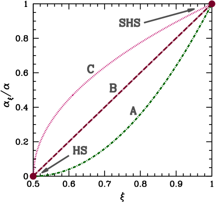
Figure 1: (Color online) The $\alpha_{\xi}$ stickiness parameter scaled by $\alpha$, in the prescriptions A, B, and C given by Eq. (37).

Since the PY integral equation is an approximate theory, a common RDF is expected to yield different EOSs depending on the route followed. In the case of the $\mu$ route, as will be seen below, an extra source of thermodynamic inconsistency arises: the EOS depends on the choice for the protocol $\alpha_{\xi}$.

IV.1 Virial expansion

Table 1: Numerical values of the coefficients $b_{4}^{\text{HS}}$ and $b_{4,i}$ [cf. Eq. (42)].

	$b_{4}^{\text{HS}}$	$b_{4,1}$	$b_{4,2}$	$b_{4,3}$	$b_{4,4}$	$b_{4,5}$	$b_{4,6}$
Exact	$18.36477$	$-165.283$	$880.416$	$-2623.10$	$3607.65$	$-1576.39$	$-194.468$
$v$	$16$	$-144$	$864$	$-2784$	$4032$	$-2304$	$0$
$e$	Undetermined	$-144$	$756$	$-2448$	$3888$	$-2073.6$	$0$
$c$	$19$	$-171$	$864$	$-2448$	$3456$	$-1728$	$0$
ZS	${5}$	${-45}$	${216}$	${-1296}$	${5184}$	${-5184}$	${0}$
$\mu_{\text{A}}$	$16.75$	$-150.75$	$853.795$	$-2711.64$	$4097.84$	$-2208.61$	$0$
$\mu_{\text{B}}$	$16.75$	$-150.75$	$860.384$	$-2737.15$	$4094.45$	$-2234.15$	$0$
$\mu_{\text{C}}$	$16.75$	$-150.75$	$866.194$	$-2759.45$	$4090.70$	$-2261.45$	$0$

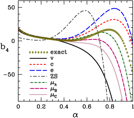
Figure 2: (Color online) Comparison of the exact fourth virial coefficient $b_{4}(\alpha)$ with the PY predictions in the virial ($v$), energy ($e$), compressibility ($c$), zero-separation (ZS), and chemical-potential ($\mu_{\text{A}}$, $\mu_{\text{B}}$, and $\mu_{\text{C}}$) routes.

Table 2: Numerical values of the coefficients $b_{5}^{\text{HS}}$ and $b_{5,i}$ [cf. Eq. (47)].

	$b_{5}^{\text{HS}}$	$b_{5,1}$	$b_{5,2}$	$b_{5,3}$	$b_{5,4}$	$b_{5,5}$	$b_{5,6}$	$b_{5,7}$
$v$	$22$	$-264$	$2700$	$-16\,920$	$63\,072$	$-134\,784$	$152\,064$	$-69\,120$
$e$	Undetermined	$-264$	$2160$	$-13\,104$	$51\,840$	$-120\,268.8$	$138\,240$	$-59\,245.7$
$c$	$31$	$-372$	$2916$	$-15\,048$	$50\,112$	$-100\,224$	$103\,680$	$-41\,472$
ZS	${-5.6}$	${67.2}$	${86.4}$	${-3974.4}$	${29\,030.4}$	${-124\,416}$	${248\,832}$	${-165\,888}$
$\mu_{\text{A}}$	$23.8$	$-285.6$	$2680.78$	$-16\,322.8$	$61\,654.4$	$-135\,696.4$	$152\,203.3$	$-65\,563.1$
$\mu_{\text{B}}$	$23.8$	$-285.6$	$2715.20$	$-16\,592.7$	$62\,400.3$	$-136\,366.0$	$153\,001.7$	$-66\,620.8$
$\mu_{\text{C}}$	$23.8$	$-285.6$	$2745.36$	$-16\,831.5$	$63\,063.1$	$-136\,973.3$	$153\,850.2$	$-67\,765.8$

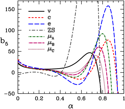
Figure 3: (Color online) Fifth virial coefficient $b_{5}(\alpha)$ as predicted by the PY theory in the virial ($v$), energy ($e$), compressibility ($c$), zero-separation (ZS), and chemical potential ($\mu_{\text{A}}$, $\mu_{\text{B}}$, and $\mu_{\text{C}}$) routes.

A standard method of examining different approximations in statistical mechanics is to compare the successive terms in the virial expansion of the compressibility factor. For SHS fluids,

$$Z(\eta,\alpha)=1+\sum_{j=2}^{\infty}b_{j}(\alpha)\eta^{j-1}.$$ (38)

The virial coefficients $b_{j}(\alpha)$ in the virial, energy, compressibility, and chemical-potential routes can be respectively evaluated from Eqs. (59), (65), (63), and (IV), complemented by the PY results summarized in Appendix D. The virial coefficients corresponding to an additional route, the so-called ZS route Barboy and Tenne (1976, 1979), can be derived within the PY approximation from Eq. (85).

All the routes in the PY approximation yield the exact second virial coefficient:

$$b_{2}(\alpha)=4-12\alpha.$$ (39)

As for the third virial coefficient, its exact expression,

$$b_{3}(\alpha)=10-60\alpha+144\alpha^{2}-96\alpha^{3},$$ (40)

is recovered from the virial, energy, compressibility, and chemical-potential routes, but not from the ZS route. The ZS result is

$${b_{3}^{(\text{ZS})}(\alpha)=-\frac{4}{3}+8\alpha+96\alpha^{2}-192\alpha^{3},}$$ (41)

which is especially wrong in the HS limit ($\alpha\to 0$).

The exact fourth virial coefficient is a sixth-degree polynomial in $\alpha$ Post and Glandt (1986), i.e.,

$$b_{4}(\alpha)=b_{4}^{\text{HS}}+\sum_{i=1}^{6}b_{4,i}\alpha^{i},$$ (42)

where the numerical coefficients are given by the first row of Table 1. The PY predictions for $b_{4}(\alpha)$ depend on the thermodynamic route. They have the structure of Eq. (42), except that $b_{4,6}=0$. The corresponding numerical coefficients are displayed in Table 1. Note that the energy route is unable to fix the HS EOS, so that the coefficients $b_{j}^{\text{HS}}$ remain undetermined in that route. All the coefficients $b_{4,i}$ derived from the $\mu$ route are rational numbers although a limited number of digits is shown in Table 1. Note that the three protocols of the $\mu$ route agree in the values of $b_{4}^{\text{HS}}=\frac{67}{4}$ and $b_{4,1}=-\frac{603}{4}$. However, the coefficients $b_{4,2}$–$b_{4,5}$ depend on the choice of $\alpha_{\xi}$. For an arbitrary function $\alpha_{\xi}$, they are

$$b_{4,2}^{(\mu)}=837\left[1+\frac{12}{31}\int_{\frac{1}{2}}^{1}\text{d}\xi\,\left(\xi^{2}-\frac{1}{4}\right)\frac{\xi^{2}\alpha_{\xi}^{2}}{\alpha^{2}}\right],$$ (43)

$$b_{4,3}^{(\mu)}=-2646\left[1+\frac{24}{49}\int_{\frac{1}{2}}^{1}\text{d}\xi\,\left(\xi^{2}+\frac{\xi^{2}\alpha_{\xi}}{6\alpha}-\frac{3}{8}\right)\frac{\xi^{2}\alpha_{\xi}^{2}}{\alpha^{2}}\right],$$ (44)

$$b_{4,4}^{(\mu)}=4104\left[1-\frac{3}{19}\int_{\frac{1}{2}}^{1}\text{d}\xi\,\left(1-\frac{4\xi^{2}\alpha_{\xi}}{3\alpha}\right)\frac{\xi^{2}\alpha_{\xi}^{2}}{\alpha^{2}}\right],$$ (45)

$$b_{4,5}^{(\mu)}=-2160\left(1+\frac{2}{5}\int_{\frac{1}{2}}^{1}\text{d}\xi\,\frac{\xi^{4}\alpha_{\xi}^{3}}{\alpha^{3}}\right).$$ (46)

The three protocols in Eq. (37) have the common form $\alpha_{\xi}=(2\xi-1)^{q}\alpha$ with $q=0.5$, $1$, and $2$ for C, B, and A, respectively. Taking $q>0$ as a free parameter and using Eqs. (43)–(46), it is possible to find the optimal value of $q$ that makes $b_{4}^{(\mu)}(\alpha)=b_{4}^{\text{exact}}(\alpha)$ for a given value $\alpha>0.282$. For instance, the optimal values are $q=0.199$, $1.208$, $2.076$, $3.702$, and $4.997$ for $\alpha=0.3$, $0.5$, $0.7$, $0.9$, and $1$, respectively. For $\alpha<0.282$ the mathematical solutions of $b_{4}^{(\mu)}(\alpha)=b_{4}^{\text{exact}}(\alpha)$ are $q<0$, but these are nonphysical values violating the condition $\alpha_{\frac{1}{2}}=0$.

Figure 2 compares the exact $b_{4}(\alpha)$ with various PY routes, where the Carnahan–Starling (CS) Hansen and McDonald (2006) value $b_{4}^{\text{HS}}=18$ has been taken in the case of the energy route. A very poor behavior of the ZS route is observed. In what concerns the other four routes, small deviations occur among them for low and moderate stickiness ($\alpha\lesssim 0.35$), a good agreement with the exact values being found in that range. For $\alpha\gtrsim 0.35$, however, larger discrepancies occur, with the energy and virial routes showing the most extreme deviations with respect to the exact solution. The $\mu$ route predictions lie between the virial and the compressibility ones, becoming closer to the exact values as a softer stickiness prescription is used (protocol A).

Although, to the best of our knowledge, the fifth virial coefficient is not exactly known, it is worthwhile comparing the different PY predictions for it. They have the polynomial structure

$$b_{5}(\alpha)=b_{5}^{\text{HS}}+\sum_{i=1}^{7}b_{5,i}\alpha^{i},$$ (47)

the coefficients being presented in Table 2. Again, all the coefficients are rational numbers. The dependence of $b_{5}(\alpha)$ on the stickiness parameter is shown in Fig. 3 (with the CS choice $b_{5}^{\text{HS}}=28$ for the energy route). As expected, the influence of the thermodynamic route on $b_{5}(\alpha)$ is stronger than in the case of $b_{4}(\alpha)$. The general shapes of $b_{5}$ in the $\mu$ and compressibility routes are intermediate between those in the virial and energy routes.

IV.2 Weakly sticky limit

Table 3: Expressions for $Z_{\text{HS}}(\eta)$ and the coefficients ${Z}_{1}(\eta)$ and ${Z}_{2}(\eta)$ [cf. Eq. (48)].

	$Z_{\text{HS}}(\eta)$	${Z}_{1}(\eta)$	${Z}_{2}(\eta)$
$v$	$\frac{1+2\eta+3\eta^{2}}{(1-\eta)^{2}}$	$-\frac{12\eta(1+2\eta)}{(1-\eta)^{3}}$	$\frac{36\eta^{2}(2+\eta)(2+3\eta)}{(1-\eta)^{4}}$
$e$	Undetermined	$-\frac{12\eta(1+2\eta)}{(1-\eta)^{3}}$	$\frac{36\eta^{2}(4+5\eta)}{(1-\eta)^{4}}$
$c$	$\frac{1+\eta+\eta^{2}}{(1-\eta)^{3}}$	$-\frac{3\eta(2+\eta)^{2}}{(1-\eta)^{4}}$	$\frac{36\eta^{2}(2+\eta)^{2}}{(1-\eta)^{5}}$
ZS	${-\frac{\ln\left[(1+2\eta)(1-\eta)^{4}\right]}{\eta}-1}$	${-3\frac{\ln\left[(1+2\eta)(1-\eta)^{4}\right]}{\eta}-\frac{6(1+5\eta)}{(1-\eta)(1+2\eta)}}$	${-3\frac{\ln\left[(1+2\eta)^{5}(1-\eta)^{64}\right]}{\eta}-\frac{18(9+25\eta-17\eta^{2}-71\eta^{3})}{(1-\eta)^{2}(1+2\eta)^{2}}}$
$\mu_{\text{A}}$	$-9\frac{\ln(1-\eta)}{\eta}-\frac{16-31\eta}{2(1-\eta)^{2}}$	$-27\frac{\ln(1-\eta)}{\eta}-\frac{3(18-37\eta+49\eta^{2})}{2(1-\eta)^{3}}$	$-648\frac{\ln(1-\eta)}{\eta}-\frac{9(8064-28\,224\eta+33\,152\eta^{2}-20\,257\eta^{3})}{112(1-\eta)^{4}}$
$\mu_{\text{B}}$	$-9\frac{\ln(1-\eta)}{\eta}-\frac{16-31\eta}{2(1-\eta)^{2}}$	$-27\frac{\ln(1-\eta)}{\eta}-\frac{3(18-37\eta+49\eta^{2})}{2(1-\eta)^{3}}$	$-\frac{96\,363}{140}\frac{\ln(1-\eta)}{\eta}-\frac{27(7138-24\,983\eta+29\,438\eta^{2}-17\,820\eta^{3})}{280(1-\eta)^{4}}$
$\mu_{\text{C}}$	$-9\frac{\ln(1-\eta)}{\eta}-\frac{16-31\eta}{2(1-\eta)^{2}}$	$-27\frac{\ln(1-\eta)}{\eta}-\frac{3(18-37\eta+49\eta^{2})}{2(1-\eta)^{3}}$	$-\frac{28\,917}{40}\frac{\ln(1-\eta)}{\eta}-\frac{9(6426-22\,491\eta+26\,566\eta^{2}-15\,967\eta^{3})}{80(1-\eta)^{4}}$

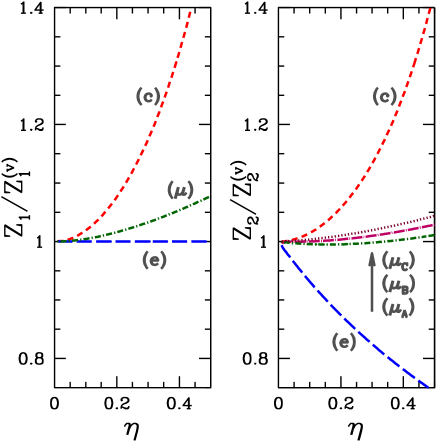
Figure 4: (Color online) Coefficients $Z_{1}(\eta)$ and $Z_{2}(\eta)$ in the $\alpha$ expansion of $Z(\eta,\alpha)$ [cf. Eq. (48)] from the PY equation in the energy ($e$), compressibility ($c$), and chemical-potential ($\mu_{\text{A}}$, $\mu_{\text{B}}$, and $\mu_{\text{C}}$) routes, relative to the coefficients $Z_{1}^{(v)}(\eta)$ and $Z_{2}^{(v)}(\eta)$ obtained in the virial route.

As a complement of the virial expansion (38), it is of interest to examine the leading terms in the series expansion

$$Z(\eta,\alpha)=Z_{\text{HS}}(\eta)+\sum_{i=1}^{\infty}{Z}_{i}(\eta)\alpha^{i}$$ (48)

of the compressibility factor in powers of the stickiness parameter. Obviously, the zeroth-order coefficient in the $\alpha$ expansion is just the compressibility factor of the pure HS system. Equation (48) can be interpreted as a high-temperature expansion.

Making use of the results of Appendix D in Eqs. (59), (65), (63), (85), and (IV), the first-order and second-order coefficients from the different routes can be derived. The results are displayed in Table 3. Interestingly, one has $Z_{1}^{(v)}(\eta)=Z_{1}^{(e)}(\eta)$, thus generalizing the results $b_{4,1}^{(v)}=b_{4,1}^{(e)}$ and $b_{5,1}^{(v)}=b_{5,1}^{(e)}$ observed in Tables 1 and 2. This reinforces that the natural extension of the energy route to HS fluids is the virial EOS Santos (2005, 2006).

The HS EOS $Z_{\text{HS}}^{(\mu)}(\eta)$ was already derived in Ref. Santos (2012). We observe that $Z_{1}^{(\mu)}(\eta)$ is protocol-independent. This generalizes to any order in density the behavior observed for $b_{4,1}^{(\mu)}$ and $b_{5,1}^{(\mu)}$ in Tables 1 and 2, respectively. The expression of $Z_{2}^{(\mu)}(\eta)$ for arbitrary $\alpha_{\xi}$ is

$$Z_{2}^{(\mu)}(\eta)= -540\frac{\ln(1-\eta)}{\eta}-\frac{18(30-105\eta+122\eta^{2}-77\eta^{3})}{(1-\eta)^{4}}$$

$$-3888\int_{\frac{1}{2}}^{1}\text{d}\xi\,\xi^{2}\left(\xi-\frac{1}{2}\right)\left(\xi-\frac{1}{6}\right)\Bigg{[}\frac{\ln(1-\eta)}{\eta}$$

$$+\frac{1-\frac{7}{2}\eta+\frac{13}{3}\eta^{2}-\frac{13\xi-\frac{11}{6}}{6\xi-1}\eta^{3}}{(1-\eta)^{4}}\Bigg{]}\frac{\alpha_{\xi}^{2}}{\alpha^{2}}.$$ (49)

The coefficients $Z_{1}(\eta)$ and $Z_{2}(\eta)$, relative to the virial-route predictions, obtained from various PY routes (except the ZS one, in order to avoid distortion of the scales) are shown in Fig. 4. The discrepancies grow as density increases. In particular, the largest inconsistencies occur between the energy and compressibility routes. On the other hand, the $\mu$ route deviates only slightly from the virial route, especially in the case of $Z_{2}$.

IV.3 Finite density and stickiness

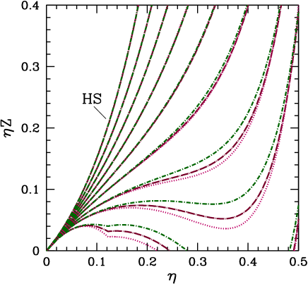
Figure 5: (Color online) Reduced pressure $\eta Z^{(\mu)}$ of SHS fluids, as obtained from the PY solution in the $\mu$ route according to the protocols A (-$\,\cdot\,$-$\,\cdot\,$-$\,\cdot$), B (—$\,\cdot\,$—$\,\cdot\,$—$\,\cdot$), and C ($\cdots\cdots$). The values of $\alpha$ are (from left to right) $\alpha=0$, $0.1$, $0.2$, $0.3$, $0.4$, $0.5$, $\alpha_{c}^{(v)}\simeq 0.612\,418$, $\alpha_{c}^{(e)}\simeq 0.703\,209$, and $\alpha_{c}^{(c)}\simeq 0.853\,553$.

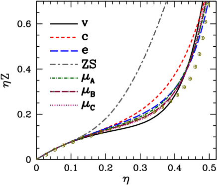
Figure 6: (Color online) Reduced pressure $\eta Z$ as a function of the packing fraction for SHS fluids at $\alpha=\frac{5}{9}\simeq 0.556$ ($\tau=\frac{3}{20}=0.15$). The curves correspond to PY results from various routes as indicated on the plot. Open circles represent MC calculations Miller and Frenkel (2004).

After having examined the low-density and low-stickiness (or high-temperature) regimes, we now consider the full non-perturbative regime. The density dependence of the reduced pressure $\eta Z^{(\mu)}$ is plotted in Fig. 5 for different values of $\alpha$ and for the three protocols (37). Of course, in the limit of zero stickiness ($\alpha=0$), the choice of the protocol becomes irrelevant and one recovers the EOS $Z^{(\mu)}_{\rm HS}(\eta)$ (see Table 3) corresponding to the PY theory in the $\mu$ route Santos (2012). As $\alpha$ increases, the pressure decreases with respect to the HS value and the influence of the protocol is practically negligible up to $\alpha\approx 0.5$. For higher stickiness, however, the values of $Z^{(\mu)}$ are increasingly sensitive to the protocol chosen. We observe that, as expected on physical grounds, the stronger the relative stickiness $\alpha_{\xi}/\alpha$, the smaller the pressure.

The three higher values of $\alpha$ in Fig. 5 correspond to the gas-liquid critical values $\alpha_{c}^{(v)}$, $\alpha_{c}^{(e)}$, and $\alpha_{c}^{(c)}$ predicted by the PY approximation in the virial, energy, and compressibility routes, respectively (see below). In fact the kink in $Z^{(\mu)}$ at $\alpha=\alpha_{c}^{(c)}$ and $\eta=\eta_{c}^{(c)}\simeq 0.12132$ reflects the fact that $(\eta_{c}^{(c)},\alpha_{c}^{(c)})$ is the critical point for the existence of real solutions of the PY equation (see Appendix D).

In Fig. 6 we compare MC simulations at $\alpha=\frac{5}{9}$ Miller and Frenkel (2004) with PY predictions from the different routes. Since, as discussed before, the energy route leaves the integration constant $Z_{\text{HS}}(\eta)$ undetermined, henceforth the CS EOS Hansen and McDonald (2006)

$$Z_{\text{HS}}^{\text{CS}}(\eta)=\frac{1+\eta+\eta^{2}-\eta^{3}}{(1-\eta)^{3}}$$ (50)

will be taken to complete the determination of $Z^{(e)}(\eta,\alpha)$ via Eq. (63), despite the fact that the choice $Z_{\text{HS}}^{(e)}=Z_{\text{HS}}^{(v)}$ would be more consistent Santos (2005, 2006). The virial, compressibility, and ZS data have been obtained from Eqs. (59), (65), and (85), respectively. In all the cases, use has been made of the PY solution detailed in Appendix D.

We observe that in the low-density range ($\eta\lesssim 0.15$) all PY routes and simulation data agree very well. For higher densities, the ZS pressure grows too rapidly and the curves corresponding to the three different protocols of the $\mu$ route remain rather close in comparison with those from the virial, energy, and compressibility routes, which show a larger spread. In the range $0.2\lesssim\eta\lesssim 0.4$, the $\mu$ route gives the best fits to the simulation data. In the same region, $Z^{(e)}$ and $Z^{(c)}$ overestimate the simulation values, while $Z^{(v)}$ underestimates them. Up to $\eta\approx 0.4$, one has $Z^{(v)}<Z^{(\mu_{\text{C}})}<Z^{(\mu_{\text{B}})}<Z^{(\mu_{\text{A}})}<Z^{(e)}<Z^{(c)}$. Finally, there is a rather strong disagreement of all the PY routes at high densities, $0.4\lesssim\eta\lesssim 0.5$, where the simulation data exhibit lower pressure values than the theoretical ones. Aside from the ZS curve, the compressibility route shows the largest deviations from MC results on the whole range of studied densities.

IV.4 Gas-liquid transition

Table 4: Comparison of the SHS gas-liquid critical values of $\alpha$, $\eta$, $\tau=1/12\alpha$, and $\rho=6\eta/\pi$ from MC simulations Miller and Frenkel (2004) and PY solutions in the virial, energy, compressibility, and chemical-potential routes.

	MC	$v$	$e$	$c$	ZS	$\mu_{\text{A}}$	$\mu_{\text{B}}$	$\mu_{\text{C}}$
$\alpha_{c}$	$0.7355$	$0.6124$	$0.7032$	$0.8536$	${0.7112}$	$0.6858$	$0.6605$	$0.6412$
$\tau_{c}$	$0.1133$	$0.1361$	$0.1185$	$0.0976$	${0.1172}$	$0.1215$	$0.1262$	$0.1300$
$\eta_{c}$	$0.2660$	$0.2524$	$0.3187$	$0.1213$	${0.1039}$	$0.2761$	$0.2691$	$0.2645$
$\rho_{c}$	$0.5080$	$0.4820$	$0.6086$	$0.2317$	${0.1985}$	$0.5274$	$0.5140$	$0.5051$

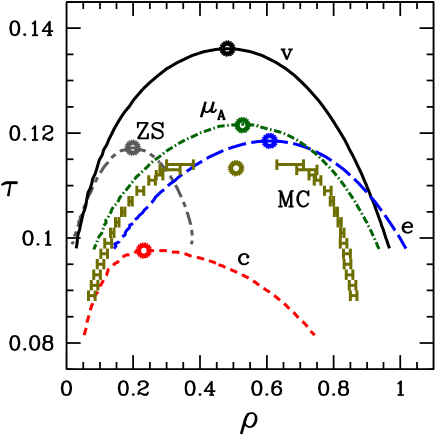
Figure 7: (Color online) Phase diagram of the SHS fluid showing the gas-liquid coexistence curves from PY solutions in the virial (—), energy (– – –), compressibility (- - -), ZS (– - – -), and chemical-potential (-$\,\cdot\,$-$\,\cdot\,$-$\,\cdot$) routes. Results in the $\mu$ route are based on prescription A. MC simulation data taken from Ref. Miller and Frenkel (2004) are shown with error bars. The critical points are indicated with circles.

The two highest values of $\alpha$ in Fig.  5 show a domain of mechanical instability, $\partial(\eta Z)/\partial\eta<0$ (i.e., $\partial p/\partial\rho<0$), which indicates a phase transition according to the $\mu$ route in the various protocols analyzed. As is well known, the SHS fluid has a (metastable) fluid-fluid transition which was early predicted in the compressibility Baxter (1968) and energy Watts et al. (1971) routes of the PY approximation. Critical values of the parameters $\alpha$ and $\eta$ (or $\tau$ and $\rho$) can be determined by the conditions $\partial p/\partial\rho=0$ and $\partial^{2}p/\partial\rho^{2}=0$. Results concerning to various PY routes are summarized in Table 4, where they can be compared to the ones obtained by Miller and Frenkel Miller and Frenkel (2004) using MC simulations.

As is known, the compressibility route produces a gross underestimation of the critical density. An even higher underestimation of $\eta_{c}$ is obtained from the ZS method. The critical density is much better approximated by the virial route (deviation of $5\%$) and, especially, the $\mu$ route (deviations of $4\%$, $1.2\%$, and $0.6\%$ for protocols A, B, and C, respectively). On the other hand, the critical value of the stickiness parameter evaluated from the virial and the compressibility routes differ significantly from those predicted by numerical experiments. For this parameter, the ZS route (deviation of $3\%$), the energy route (deviation of $4\%$) and the $\mu$ route (deviations of $7\%$, $10\%$, and $13\%$ for A, B, and C, respectively) give the best results. In view of the general poor performance of the ZS route, its good prediction of the critical stickiness can be viewed as accidental. In addition, it must be remarked that the critical point obtained from $Z^{(e)}$ is quite sensitive to the choice of $Z_{\text{HS}}$. If, instead of the CS EOS (50), the more consistent choice Santos (2005, 2006) $Z_{\text{HS}}=Z_{\text{HS}}^{(v)}$ is used, then no SHS critical point is predicted by the energy route. In conclusion, the parameters of the critical points obtained from the $\mu$ route show the best global agreement with simulations.

We have also computed coexistence curves with the familiar equal-area Maxwell construction that is applicable when $\partial p/\partial\rho<0$. Figure 7 displays the coexistence curve and the location of the critical point derived by various PY routes and from computer simulations Miller and Frenkel (2004). For simplicity, in the case of the $\mu$ route only results from protocol A are shown. As may be seen in Fig. 7, the curves obtained from the virial, compressibility, and ZS routes differ substantially from computer evaluations. On the contrary, the agreement is reasonably good for the energy and $\mu$ routes. As already seen from Table 4, the critical Baxter temperature $\tau_{c}$ predicted by the energy route is more accurate than the one obtained from the $\mu$ route. However, the general shape of the coexistence curve (both the gas and the liquid branches) is better described by the $\mu$ route.

V Conclusions

In this paper we have studied the SHS fluid using the concept of a partially coupled particle, whereby the interaction potential connecting this particle (the solute) to all other particles in the fluid (the solvent) is regulated by a charging parameter $\xi$ which varies from $\xi=0$ (no interaction) to $\xi=1$ (full interaction). With this method, first introduced by Onsager Onsager (1933) and subsequently developed by Kirkwood Kirkwood (1935) and other authors Hill (1956); Reiss et al. (1959), we have derived the chemical potential of $d$-dimensional SHS fluids in terms of the contact values of the solute-solvent cavity function $y_{\xi}(\xi)$ and its first derivative $y^{\prime}_{\xi}(\xi)$ [see Eqs. (24) and (22)].

The procedure requires $y_{\xi}(\xi)$ and $y^{\prime}_{\xi}(\xi)$ in the range $\frac{1}{2}<\xi<1$, where the effective diameter ($2\xi-1$) of the coupled particle varies between zero to the solute diameter $\sigma=1$. Thus, the explicit evaluation of the EOS of the fluid in the $\mu$ route requires the structural functions of the corresponding binary system in the infinite dilution limit. While this may represent a practical disadvantage with respect to the other standard routes (which only require the RDF of the one-component fluid), it nicely complements them. As is well known, the natural variables of the free energy $F$ are the temperature ($T$), the volume ($V$), and the number of particles ($N$). The internal energy, the pressure and the isothermal compressibility are directly related to $\partial F/\partial T$, $\partial F/\partial V$, and $\partial^{2}F/\partial V^{2}$, respectively. Therefore, the chemical potential, being related to $\partial F/\partial N$, completes the picture.

The $\mu$ route also requires a prescription for the solute-solvent interaction potential, i.e., the dependence of the solute-solvent stickiness $\alpha_{\xi}$ on the coupling parameter $\xi$ must be specified. Here, in order to avoid the effects of trimer particle configurations, we have selected prescriptions with $\alpha_{\xi}=0$ at $\xi=\frac{1}{2}$. The resulting EOS, Eq. (26), is exact if the correct contact values $y_{\xi}(\xi)$ and $y^{\prime}_{\xi}(\xi)$ are used, regardless of the explicit form of $\alpha_{\xi}$ in the range $\frac{1}{2}<\xi\leq 1$. This has been checked for the one-dimensional sticky fluid, in which case the exact EOS is recovered from the $\mu$ route (see Sec. III).

We have also applied the $\mu$ route to three-dimensional SHS fluids in the PY approximation. In this case, since the associated RDF is only approximate, the $\mu$ route EOS is influenced by the choice of the $\alpha_{\xi}$-protocol. On the other hand, this thermodynamical inconsistency becomes small in comparison with the spread of results obtained from the other routes (virial, energy, compressibility, and ZS). When compared with available simulation data Miller and Frenkel (2004), the $\mu$ route EOS exhibits a general better agreement than those evaluated from the other routes. The gas-liquid phase transition has also been analyzed. The $\mu$ route provides the best prediction for the critical density, being only improved by the ZS and energy routes in the prediction of the critical stickiness parameter. To put this latter fact in perspective, it is important to remark that, as usually done Watts et al. (1971), the energy route has been complemented ad hoc by the accurate CS EOS for the HS fluid. As for the coexistence curve, the best global agreement with simulation data is obtained from the $\mu$ route. In addition, comparison of the fourth virial coefficient with exact results shows that the best performance corresponds to the $\mu$ route with a slower switching on of stickiness (protocol A).

To conclude, we expect that the results presented in this paper may contribute to place the $\mu$ route on the same footing as the other three conventional routes. This is especially important in the case of mixtures Santos and Rohrmann (2013), where the chemical-potential concept fits in a more natural way. Regarding the PY approximation, it is interesting to note that, whereas in the case of the HS fluid Santos (2012); Santos and Rohrmann (2013) the best behavior corresponds to the compressibility route (followed by the $\mu$ route), the inclusion of an attractive part in the interaction potential seems to favor the $\mu$ route as the most advantageous one.

Appendix A The limit $\xi\to\frac{1}{2}$

In contrast to the situation with $\xi<\frac{1}{2}$, a solute particle with $\xi=\frac{1}{2}$ allows spatial configurations where the solute and two solvent particles are simultaneously touching each other. Such configurations have a non-zero statistical weight in the evaluation of Eq. (7) through the term of order $\alpha_{\xi}^{2}$ in Eq. (II), unless $\alpha_{\frac{1}{2}}=0$. Such a term is

$$Q_{N+1}^{(\frac{1}{2},2)}\equiv \frac{\alpha_{\frac{1}{2}}^{2}}{4V^{N+1}}\int\text{d}\mathbf{r}^{N}e^{-\beta\Phi_{N}(\mathbf{r}^{N})}\int\text{d}\mathbf{r}_{0}\sum_{i\neq j}^{N}\delta\left(r_{0i}-\frac{1}{2}\right)$$

$$\times\delta\left(r_{0j}-\frac{1}{2}\right)\prod_{k\neq i,j}\Theta\left(r_{0k}-\frac{1}{2}\right)$$

$$= \alpha_{\frac{1}{2}}^{2}\frac{N(N-1)}{4V^{N+1}}\int\text{d}\mathbf{r}^{N}e^{-\beta\Phi_{N}(\mathbf{r}^{N})}$$

$$\times\int\text{d}\mathbf{r}_{0}\,\delta\left(r_{01}-\frac{1}{2}\right)\delta\left(r_{02}-\frac{1}{2}\right),$$ (51)

where we have taken into account that, if $r_{0i}=r_{0j}=\frac{1}{2}$, one has $r_{0k}>\frac{1}{2}$ $\forall k\neq i,j$. Next, $r_{01}=r_{02}=\frac{1}{2}$ is compatible with $r_{12}\geq 1$ only if $r_{12}=1$. Thus, using spherical coordinates,

$$Q_{N+1}^{(\frac{1}{2},2)} =\alpha_{\frac{1}{2}}^{2}\frac{d}{8}\Omega_{\frac{1}{2}}\frac{N(N-1)}{V^{N+1}}\int\text{d}\mathbf{r}^{N}e^{-\beta\Phi_{N}(\mathbf{r}^{N})}\delta(r_{12}-1)$$

$$=\alpha_{\frac{1}{2}}^{2}\frac{d}{8}\rho^{2}\Omega_{\frac{1}{2}}Q_{N}\int\text{d}\mathbf{r}\,\delta(r-1)g(r),$$ (52)

where

$$g(r_{12})=\frac{V^{-(N-2)}}{Q_{N}}\int\text{d}\mathbf{r}_{3}\cdots\int\text{d}\mathbf{r}_{N}e^{-\beta\Phi_{N}(\mathbf{r}^{N})}$$ (53)

is the solvent RDF. Finally, introducing the solvent cavity function

$$y(r)\equiv g(r)e^{\beta\phi(r)}$$ (54)

and using Eq. (3), we obtain

$$Q_{N+1}^{(\frac{1}{2},2)}=\alpha_{\frac{1}{2}}^{2}d^{2}2^{d-3}\eta^{2}y(1)Q_{N}\lim_{r\to 1}\left[\Theta(r-1)+\alpha\delta(r-1)\right],$$ (55)

where $\eta$ is defined by Eq. (16). This contribution is singular by a two-fold reason. First, the Heaviside function implies that the result depends on whether $\xi\to\frac{1}{2}$ from below or from above. Second, and more importantly, the $\delta$ function gives a divergent term. Both singularities are avoided by the choice $\alpha_{\frac{1}{2}}=0$.

Appendix B Virial, energy, and compressibility routes

For systems of particles interacting through two-body central forces, the thermodynamic functions can be evaluated in terms of the RDF $g(r)$. In particular, the pressure $p$, the excess internal energy per particle $u^{\rm ex}$, and the isothermal susceptibility $\chi$ are given by Hill (1956); Balescu (1974); Barker and Henderson (1976); Hansen and McDonald (2006)

$$p=\rho kT-\frac{\rho^{2}}{2d}\int\text{d}\mathbf{r}\,\frac{\partial\phi(r)}{\partial r}rg(r),$$ (56)

$$u^{\rm ex}=\frac{\rho}{2}\int\text{d}\mathbf{r}\,\phi(r)g(r),$$ (57)

$$\chi\equiv{k_{B}T}\left(\frac{\partial\rho}{\partial p}\right)_{T}=1+\rho\int\text{d}\mathbf{r}\,[g(r)-1].$$ (58)

Equations (56), (57), and (58) are usually known as the pressure (or virial), energy, and compressibility equations, respectively.

For SHS fluids, the compressibility factor, $Z\equiv p/\rho kT$, can be expressed from Eqs. (56) and (1) in terms of the contact values of the cavity function and its radial derivative $y^{\prime}(r)$ as

$$Z^{(v)}(\eta,\alpha)=1+2^{d-1}\eta\{y(1)-\alpha[dy(1)+y^{\prime}(1)]\}.$$ (59)

Here, the superscript $v$ specifies that the compressibility factor proceeds from the virial equation.

In turn, the excess of internal energy per particle is related with the compressibility factor as follows:

$$\rho\frac{\partial u^{\rm ex}}{\partial\rho}=-k_{B}T^{2}\frac{\partial Z}{\partial T}.$$ (60)

For SHS fluids, the changes of variables $\rho\rightarrow\eta$ and $T\rightarrow\alpha$ yield

$$\eta\frac{\partial u^{\rm ex}/\epsilon}{\partial\eta}=\alpha\frac{\partial Z}{\partial\alpha},$$ (61)

where we have taken into account that, according to Eq. (2), $\partial_{T}=-(\epsilon\alpha/k_{B}T^{2})\partial_{\alpha}$. Moreover, the excess energy can be expressed from Eq. (57) in terms of the cavity function using Eqs. (54) and (1):

$$\frac{u^{\rm ex}}{\epsilon}=-d{2^{d-1}}\eta\alpha y(1).$$ (62)

Integration of Eq. (61) with (62) yields the compressibility factor in the energy route as

$$Z^{(e)}(\eta,\alpha)=Z_{\rm HS}(\eta)-{d2^{d-1}}\eta\int_{0}^{\alpha}\text{d}\alpha^{\prime}\,\left(\frac{\partial[\eta y(1)]}{\partial\eta}\right)_{\alpha^{\prime}},$$ (63)

where $Z_{\rm HS}(\eta)$ is the compressibility factor for pure HS (which here remains undetermined) and in the integrand $y(1)$ is a function of $\eta$ and $\alpha^{\prime}$.

As for the compressibility route, taking into account that $\chi^{-1}=\left({\partial\eta Z}/{\partial\eta}\right)_{T}$ and introducing the moments

$$H_{n}\equiv\int_{0}^{\infty}\text{d}r\,r^{n}h(r)$$ (64)

of the total correlation function $h(r)=g(r)-1$, one can find

$$Z^{(c)}(\eta,\alpha)=\int_{0}^{1}\frac{\text{d}t}{\chi(\eta t)}=\int_{0}^{1}\frac{\text{d}t}{1+d2^{d}\eta H_{d-1}(\eta t)}.$$ (65)

Appendix C RDF of sticky hard rods

The exact solution of one-dimensional ($d=1$) fluids with nearest-neighbor interactions is well known Salsburg et al. (1953); Lebowitz and Zomick (1971); Heying and Corti (2004); Santos (2007); not . In the case of an infinitely diluted solute particle in a solvent, the Laplace transform

$$G_{\xi}(s)=\int_{0}^{\infty}\text{d}r\,e^{-rs}g_{\xi}(r)$$ (66)

of the RDF $g_{\xi}(r)$ is given by

$$G_{\xi}(s)=\frac{1}{\rho}\frac{\Psi_{\xi}(s+\beta p)/\Psi_{\xi}(\beta p)}{1-\Psi(s+\beta p)/\Psi(\beta p)},$$ (67)

where $\Psi(s)$ and $\Psi_{\xi}(s)$ are the Laplace transforms of $e^{-\beta\phi(r)}$ (solvent-solvent interaction) and $e^{-\beta\phi_{\xi}(r)}$ (solute-solvent interaction), respectively.

In the particular case of sticky hard rods, use of Eqs. (1) and (3) gives

$$\Psi(s)=\left(\frac{1}{s}+\alpha\right)e^{-s},\quad\Psi_{\xi}(s)=\left(\frac{1}{s}+\alpha_{\xi}\xi\right)e^{-s\xi}.$$ (68)

Moreover, the exact EOS is

$$\beta p=\frac{\sqrt{1+4\alpha\eta/(1-\eta)}-1}{2\alpha}.$$ (69)

Expansion of the right-hand side of Eq. (67) in powers of $e^{-s}$ allows one to obtain $g_{\xi}(r)$ in the shells $0<r<1+\xi$, $1+\xi<r<2+\xi$, $\ldots$ In particular, if $r<1+\xi$,

$$g_{\xi}(r)=\frac{\alpha_{\xi}\xi\delta(r-\xi)+e^{-\beta p(r-\xi)}\Theta(r-\xi)}{\eta(\alpha_{\xi}\xi+1/\beta p)},\quad r<1+\xi.$$ (70)

Taking into account Eqs. (3) and (20), one has

$$y_{\xi}(r)=\frac{e^{-\beta p(r-\xi)}}{\eta(\alpha_{\xi}\xi+1/\beta p)},\quad\xi\leq r<1+\xi.$$ (71)

From here one easily gets Eq. (31).

Appendix D Solution of the PY equation for SHS

In this Appendix we summarize the main results obtained from the exact solution of the PY integral equation for SHS. The reader is referred to Refs. Baxter (1968); Barboy (1974); Yuste and Santos (1993a, b); Perram and Smith (1975); Barboy (1975); Barboy and Tenne (1979); Santos et al. (1998) for further details.

D.1 Solvent properties

The PY solution is expressed in terms of the Laplace transform

$$G(s)=\int_{0}^{\infty}\text{d}r\,e^{-rs}rg(r)$$ (72)

of $rg(r)$. Such a solution is

$$s^{2}e^{s}G(s)=\frac{L_{0}+L_{1}s+L_{2}s^{2}}{1-12\eta\left[\psi_{2}(s)L_{0}+\psi_{1}(s)L_{1}+\psi_{0}(s)L_{2}\right]},$$ (73)

where

$$\psi_{n}(s)\equiv\frac{1}{s^{n+1}}\left[\sum_{m=0}^{n}\frac{(-s)^{m}}{m!}-e^{-s}\right].$$ (74)

The quantities $L_{0}$, $L_{1}$, and $L_{2}$ are given as functions of $\eta$ and $\alpha$ by

$$L_{0}=\frac{1+2\eta}{(1-\eta)^{2}}-\frac{12\eta}{1-\eta}L_{2},\quad L_{1}=\frac{1+\eta/2}{(1-\eta)^{2}}-\frac{6\eta}{1-\eta}L_{2},$$ (75)

$$L_{2}=\frac{1-(1-12\alpha)\eta-K}{24\alpha(1-\eta)\eta},$$ (76)

where

$$K\equiv\sqrt{(1-\eta)[1-\eta(1-24\alpha+48\alpha^{2})]+72\alpha^{2}\eta^{2}}.$$ (77)

The large-$s$ behavior of $G(s)$ provides the contact values of $y(r)$ and $y^{\prime}(r)$. The results are

$$y(1)=\frac{L_{2}}{\alpha},$$ (78)

$$y^{\prime}(1)= -\frac{9\eta(1+\eta)}{2(1-\eta)^{3}}+\frac{12\eta(1+5\eta)}{(1-\eta)^{2}}L_{2}-\frac{12\eta(1+11\eta)}{1-\eta}L_{2}^{2}$$

$$+144\eta^{2}L_{2}^{3}.$$ (79)

Insertion of these expressions into Eq. (59) (with $d=3$) gives the virial equation

$$Z^{(v)}= \frac{1+2\eta+3\eta^{2}}{(1-\eta)^{2}}+18\alpha\frac{\eta^{2}(1+\eta)}{(1-\eta)^{2}}$$

$$-\frac{12\eta}{1-\eta}\left[1+3\eta+4\alpha\frac{\eta(1+5\eta)}{1-\eta}\right]L_{2}$$

$$+48\eta^{2}\left(1+\alpha\frac{1+11\eta}{1-\eta}\right)L_{2}^{2}-576\eta^{3}\alpha L_{2}^{3}.$$ (80)

Analogously, insertion of Eq. (78) into Eq. (63) yields an analytical expression for $Z^{(e)}-Z_{\text{HS}}$.

The moment $H_{2}$ of the total correlation function [cf. Eq. (64)] can be obtained from the small-$s$ behavior of $G(s)$ as $s^{2}G(s)=1+H_{1}s^{2}-H_{2}s^{3}+\mathcal{O}(s^{3})$. Inserting the resulting expression of $H_{2}$ into $\chi=1+24\eta H_{2}$ [cf. Eq. (58)], one obtains

$$\frac{1}{\chi}=\frac{\left[1+2\eta-12\eta(1-\eta)L_{2}\right]^{2}}{(1-\eta)^{4}}.$$ (81)

The compressibility factor $Z^{(c)}$ by the compressibility route is readily obtained in analytical form by application of Eq. (65). For conciseness, the explicit expressions of $Z^{(c)}$ and $Z^{(e)}$ will be omitted here.

As a consequence of the square root present in $K(\eta,\alpha)$ [cf. Eq. (77)], the PY solution is not physically meaningful if $\alpha>\alpha_{c}^{(c)}\equiv\frac{2+\sqrt{2}}{4}\simeq 0.85355$ (or $\tau<1/12\alpha_{c}^{(c)}=0.09763$) and $\eta_{-}(\alpha)<\eta<\eta_{+}(\alpha)$, where

$$\eta_{\pm}(\alpha)=\frac{1-12\alpha+24\alpha^{2}\pm 6\alpha\sqrt{2-16\alpha(1-\alpha)}}{1-24\alpha+120\alpha^{2}}.$$ (82)

In the limit $\alpha\to\alpha_{c}^{(c)}$ one has $\eta_{\pm}\to\eta_{c}^{(c)}=(3\sqrt{2}-4)/2\simeq 0.121\,32$. It can be easily checked that the right-hand side of Eq. (81) vanishes at $(\eta,\alpha)=(\eta_{c}^{(c)},\alpha_{c}^{(c)})$. This implies that $(\eta_{c}^{(c)},\alpha_{c}^{(c)})$ is the critical point in the compressibility route.

As an extra route, Barboy and Tenne Barboy and Tenne (1979) applied the so-called ZS theorem Barboy and Tenne (1976) to the PY solution for SHS fluids. According to this ZS route, the excess chemical potential is expressed as

$${\beta\mu^{\text{ex}}=\ln y_{\text{reg}},}$$ (83)

where

$${y_{\text{reg}}=\frac{\left[1-4\eta-(1-\eta-K)/2\alpha\right]^{2}}{(1-\eta)^{4}}}$$ (84)

is the regular part of the cavity function at $r=0$. The associated compressibility factor is then obtained from the thermodynamic relation (27), i.e.,

$${Z^{(\text{ZS})}(\eta,\alpha)=1+\ln y_{\text{reg}}(\eta,\alpha)-\int_{0}^{1}dt\,\ln y_{\text{reg}}(\eta t,\alpha)}.$$ (85)

D.2 Solute-solvent RDF

From the exact solution of the PY equation for an SHS binary mixture Perram and Smith (1975); Santos et al. (1998) one can take the limit where one of the species (the solute) is infinitely dilute. As a result, the Laplace transform

$$G_{\xi}(s)=\int_{0}^{\infty}\text{d}r\,e^{-rs}rg_{\xi}(r)$$ (86)

of $rg_{\xi}(r)$ is given by

$$s^{2}e^{s\xi}G_{\xi}(s)=\frac{L_{0}+L_{1}^{(\xi)}s+L_{2}^{(\xi)}s^{2}}{1-12\eta\left[\psi_{2}(s)L_{0}+\psi_{1}(s)L_{1}+\psi_{0}(s)L_{2}\right]},$$ (87)

where

$$L_{1}^{(\xi)}=\frac{\xi+\eta(2\xi-3/2)}{(1-\eta)^{2}}-\frac{6\eta(2\xi-1)}{1-\eta}L_{2},$$ (88)

$$L_{2}^{(\xi)}=\left(\frac{1}{\alpha_{\xi}\xi}+\frac{6\eta}{1-\eta}-12\eta L_{2}\right)^{-1}L_{1}^{(\xi)}.$$ (89)

From the large-$s$ behavior of $G_{\xi}(s)$ we can obtain the contact values of $y_{\xi}(r)$ and $y_{\xi}^{\prime}(r)$ as

$$y_{\xi}(\xi)=\frac{L_{2}^{(\xi)}}{\alpha_{\xi}\xi^{2}},$$ (90)

$$\xi y^{\prime}_{\xi}(\xi)= 12\eta L_{2}^{(\xi)}\left[3\eta\left(L_{0}-2L_{1}+2L_{2}\right)^{2}-L_{0}+L_{1}\right]$$

$$+L_{0}+6\eta L_{1}^{(\xi)}(L_{0}-2L_{1}+2L_{2})-y_{\xi}(\xi).$$ (91)

References

- Onsager (1933) L. Onsager, Chem. Rev. 13, 73 (1933).
- Kirkwood (1935) J. G. Kirkwood, J. Chem. Phys. 3, 300 (1935).
- Hill (1956) T. L. Hill, Statistical Mechanics (McGraw-Hill, New York, 1956).
- Reichl (1980) L. E. Reichl, A Modern Course in Statistical Physics (University of Texas Press, Austin, 1980), 1st ed.
- Hansen and McDonald (2006) J.-P. Hansen and I. R. McDonald, Theory of Simple Liquids (Academic, London, 2006).
- Salsburg et al. (1953) Z. W. Salsburg, R. W. Zwanzig, and J. G. Kirkwood, J. Chem. Phys. 21, 1098 (1953).
- Reiss et al. (1959) H. Reiss, H. L. Frisch, and J. L. Lebowitz, J. Chem. Phys. 31, 369 (1959).
- Lebowitz et al. (1965) J. L. Lebowitz, E. Helfand, and E. Praestgaard, J. Chem. Phys. 43, 774 (1965).
- Mandell and Reiss (1975) M. Mandell and H. Reiss, J. Stat. Phys. 13, 113 (1975).
- Heying and Corti (2004) M. Heying and D. Corti, J. Phys. Chem. B 108, 19756 (2004).
- Stillinger et al. (2006) F. H. Stillinger, P. G. Debenedetti, and S. Chatterjee, J. Chem. Phys. 125, 204504 (2006).
- Santos (2012) A. Santos, Phys. Rev. Lett. 109, 120601 (2012).
- Santos and Rohrmann (2013) A. Santos and R. D. Rohrmann, Phys. Rev. E 87, 052138 (2013).
- Beltrán-Heredia and Santos (2014) E. Beltrán-Heredia and A. Santos, J. Chem. Phys. 140, 134507 (2014).
- Baxter (1968) R. J. Baxter, J. Chem. Phys. 49, 2770 (1968).
- Barboy (1974) B. Barboy, J. Chem. Phys. 61, 3194 (1974).
- Chen et al. (1994) S. H. Chen, J. Rouch, F. Sciortino, and P. Tartaglia, J. Phys.: Condens. Matter 6, 109855 (1994).
- Verduin and Dhont (1995) H. Verduin and J. K. G. Dhont, J. Colloid Interf. Sci. 172, 425 (1995).
- Rosenbaum et al. (1996) D. Rosenbaum, P. C. Zamora, and C. F. Zukoski, Phys. Rev. Lett. 76, 150 (1996).
- Pontoni et al. (2003) D. Pontoni, S. Finet, T. Narayanan, and A. R. Rennie, J. Chem. Phys. 119, 6157 (2003).
- Buzzaccaro et al. (2007) S. Buzzaccaro, R. Rusconi, and R. Piazza, Phys. Rev. Lett. 99, 098301 (2007).
- Piazza et al. (1998) R. Piazza, V. Peyre, and V. Degiorgio, Phys. Rev. E 58, R2733 (1998).
- Noro and Frenkel (2000) M. G. Noro and D. Frenkel, J. Chem. Phys. 113, 2941 (2000).
- Maestre et al. (2013) M. A. G. Maestre, R. Fantoni, A. Giacometti, and A. Santos, J. Chem. Phys. 138, 094904 (2013).
- Perram and Smith (1975) J. W. Perram and E. R. Smith, Chem. Phys. Lett. 35, 138 (1975).
- Barboy and Tenne (1979) B. Barboy and R. Tenne, Chem. Phys. 38, 369 (1979).
- Barboy and Tenne (1976) B. Barboy and R. Tenne, Mol. Phys. 31, 1749 (1976).
- Miller and Frenkel (2004) M. A. Miller and D. Frenkel, J. Chem. Phys. 121, 535 (2004).
- Post and Glandt (1986) A. J. Post and E. D. Glandt, J. Chem. Phys. 84, 4585 (1986).
- Santos (2005) A. Santos, J. Chem. Phys. 123, 104102 (2005).
- Santos (2006) A. Santos, Mol. Phys. 104, 3411 (2006).
- Watts et al. (1971) R. O. Watts, D. Henderson, and R. J. Baxter, Adv. Chem. Phys. 21, 421 (1971).
- Balescu (1974) R. Balescu, Equilibrium and Nonequilibrium Statistical Mechanics (Wiley, New York, 1974).
- Barker and Henderson (1976) J. A. Barker and D. Henderson, Rev. Mod. Phys. 48, 587 (1976).
- Lebowitz and Zomick (1971) J. L. Lebowitz and D. Zomick, J. Chem. Phys. 54, 3335 (1971).
- Santos (2007) A. Santos, Phys. Rev. E 76, 062201 (2007).
- (37) See also A. Santos, “Radial Distribution Function for Sticky Hard Rods”, http://demonstrations.wolfram.com/RadialDistributionFunctionForStickyHardRods/, Wolfram Demonstrations Project.
- Yuste and Santos (1993a) S. B. Yuste and A. Santos, J. Stat. Phys. 72, 703 (1993a).
- Yuste and Santos (1993b) S. B. Yuste and A. Santos, Phys. Rev. E 48, 4599 (1993b).
- Barboy (1975) B. Barboy, Chem. Phys. 11, 357 (1975).
- Santos et al. (1998) A. Santos, S. B. Yuste, and M. López de Haro, J. Chem. Phys. 109, 6814 (1998).