Excitation transfer pathways in excitonic aggregates revealed by the stochastic Schrödinger equation

Abstract

We derive the stochastic Schrödinger equation for the system wave vector and use it to describe the excitation energy transfer dynamics in molecular aggregates. We suggest a quantum-measurement based method of estimating the excitation transfer time. Adequacy of the proposed approach is demonstrated by performing calculations on a model system. The theory is then applied to study the excitation transfer dynamics in a photosynthetic pigment-protein Fenna-Matthews-Olson (FMO) aggregate using both the Debye spectral density and the spectral density obtained from earlier molecular dynamics simulations containing strong vibrational high-frequency modes. The obtained results show that the excitation transfer times in the FMO system are affected by the presence of the vibrational modes, however the transfer pathways remain the same.

I introduction

Recent 2D spectroscopy studies of photosynthetic pigment-protein complexes Engel et al. (2007); Panitchayangkoon et al. (2010) have shown the evidence of coherent dynamics which may play a role in energy transfer processes. These results sparked numerous debates whether the coherent system dynamics are related to the observed high efficiency and speed of the excitation energy transfer in such systems Novoderezhkin and van Grondelle (2010); Ishizaki et al. (2010); Olaya-Castro and Scholes (2011); Mennucci and Curutchet (2011); Schlau-Cohen et al. (2011); König and Neugebauer (2012). Persistance of the coherent beats over picosecond and their robustness contradict with predictions using conventional exciton relaxation theory based on Markovian Redfield equation Pachón and Brumer (2011); Cheng and Fleming (2009). Possible vibronic contribution into some of these beats has been proposed in a number of recent studies resulting in complex behavior of the excitonic/vibronic 2D spectra Mančal et al. (2012); Christensson et al. (2012); Mančal et al. (2010). Although long lasting beats in photosynthetic complexes reported by Raman spectroscopy measurements are well known for a long time Chachisvilis et al. (1995), the Raman experiments only provide information about the ground state molecular. However, the coherent beats observed by 2D spectroscopy have contributions from the electronic excited states and hence the origin of the beats becomes obscure even in a such well-studied photosynthetic complex as Fenna-Matthews-Olson (FMO) Milder et al. (2010); Christensson et al. (2012); Kreisbeck et al. (2013). A number of experiments and theoretical studies has been recently acomplished to disentangle the electronic/vibrational origin of these beats in simple systems Butkus et al. (2012, 2013); Westenhoff et al. (2012).

The strong interaction of molecular systems to environment greatly increases the difficulty to theoretically describe the dynamics of the systems because the environment has an infinite number of degrees of freedom. Without the environment no such phenomena as relaxation or energy transfer would be possible since only the macroscopic size of the environment ensures truly irreversible dynamics of the system. The most general way to calculate the quantum system dynamics is firstly to solve the problem of the evolution of the whole closed quantum system S+B, which can be described by its density operator $\widehat{\rho}\left(t\right)$, and then to calculate the needed observables of the system S. If the Hamiltonian $\widehat{H}$ characterizes this composite system, its exact evolution in time is governed by the Liouville equation for the full density operator $\widehat{\rho}\left(t\right)$:

$$i\frac{\textrm{d}}{\textrm{d}t}\widehat{\rho}\left(t\right)=\left[\widehat{\rho}\left(t\right),\widehat{H}\right].$$ (1)

Unfortunately practically it is not possible to solve it directly. Therefore approximate methods which reduce the complexity of the open quantum system are welcome Valkunas et al. (2013); Breuer and Petruccione (2002); May and Kühn (2004); Hashitsume et al. (1992).

Usually we are interested only in the dynamics of the system S which we can describe using the reduced density operator $\widehat{\rho}_{red}\left(t\right)$. It can be obtained by averaging over the environmental degrees of freedom, i. e., performing the trace operation

$$\widehat{\rho}_{\textrm{red}}\left(t\right)=\textrm{Tr}_{\textrm{B}}\left[\widehat{\rho}\left(t\right)\right].$$ (2)

Second order perturbation theory with respect to system-bath interaction leads to the Redfield equation for the reduced density operator of the system Redfield (1957); Valkunas et al. (2013). The Redfield approach is sufficiently accurate and computationally effective for rather large systems which interact weakly with the environment. The closely related Lindblad equation Lindblad (1976); Gorini et al. (1978) method has the advantage of preserving the trace of the system reduced density operator. The Lindblad equation can describe the system dynamics at approximately the same level as Redfield equation Abramavicius and Mukamel (2010). Time-adaptive Density Matrix Renormalization Group (t-DMRG) Prior et al. (2010); Chin et al. (2011), Hierarchical Equations of Motion (HEOM) Tanimura (2006); Ishizaki and Fleming (2009a) allow to incorporate the influence of the heat bath on the system non-perturbatively. The HEOM method is formally exact for certain types of environments, thus in principle it does not have restrictions on the values of system parameters or system-bath coupling strength. However in practice HEOM is computationally very costly, therefore its application is limited only to small systems at sufficiently high temperatures. The t-DMRG approach utilizes a unitary transformation of the whole composite system into a linear 1D nearest-neighbor model. It is formally exact and allows the usage of an arbitrary environmental spectral density but it cannot include correlations between fluctuations of different molecules, which may be important in spectroscopy Abramavicius and Mukamel (2011). An iterative linearized density matrix (ILDM) stochastic approach propagates the density matrix using the path integral technique for the environment Huo and Coker (2010). Formally path integral is exact approach as well, however a simplified version of ILDM allows its practical application.

All the methods relying on the calculation of the reduced density operator share a common property which allows only the investigation of the statistically averaged behavior of the system S. However, in this case the information about the instantaneous dynamic characteristics of the system is lost. To investigate them the wavefunction description of the system is preferrable. One of the approximate approaches for the wavefunction is based on the smart guess of parametrized wavefunction (so-called ansatz). A variational method is then used to determine equations of motion for the wavefunction parameters Chorosajev et al. (2013); Sun et al. (2010); Luo et al. (2010); Ye et al. (2012) for the wavefunction to approximately satisfy the Schrödinger equation with. However, the solution is restricted to the specific domain of the ansatz. Alternative approaches for the wavefunction can be classified as quantum jump methods and quantum state diffusion methods. The quantum jump methods are based on a deterministic evolution of the system wave vector with random jumps of the system state, e. g., surface hopping when some vibrational adiabatic coordinate is explicitly included Dahlbom et al. (2002); Beenken et al. (2002) and they govern the jump rates, or where jumps are realized by explicit jump operators (so-called quantum Monte-Carlo approach) Mølmer et al. (1993); Piilo et al. (2008, 2009); Rebentrost et al. (2009a). Quantum state diffusion methods propagate the system wave vector under the influence of continuous fluctuations which represent the action of the environment Gisin and Percival (1992, 1993); Diósi et al. (1998); Broadbent et al. (2012); Zhong and Zhao (2013).

In this paper we apply the stochastic approach to study the excitation transfer times in molecular aggregates. Their histograms provide information on excitation transport pathways. The main goal of this paper is to investigate the dependency of the excitation energy transfer in the FMO complex on the intra-molecular vibrations represented by the high frequencies of the environmental spectral density. In Sec. II we will see how this wave vector can be interpreted and then we derive the general form of the stochastic Schrödinger equation (SSE). In Sec. III we define the procedure of transfer time calculation and demonstrate its validity and the accuracy of the SSE method on the simple dimer calculating the population dynamics and transfer time distributions. Further we apply the SSE to study the dynamics of the FMO complex and investigate the energy transfer dependency on the intra-molecular vibrations in Sec. IV.

II Theory

II.1 Stochastic Schrödinger equation

Let us consider a quantum system, defined by the Hamiltonian $\widehat{H}_{\textrm{S}}$. In general the operator in some particular basis $\left|n\right\rangle$ can be represented in the following bra-ket form

$$\widehat{H}_{\textrm{S}}=\overset{N}{\underset{n=1}{\sum}}\varepsilon_{n}\left|n\right\rangle\left\langle n\right|+\overset{N}{\underset{n\neq m}{\sum}}J_{nm}\left|n\right\rangle\left\langle m\right|,$$ (3)

where $N$ is the number of basis vectors (in the following we denote them as sites), $\varepsilon_{n}$ - the energy of the $n$-th site, $J_{nm}$ - the interaction energy between sites $n$ and $m$. The environment is the harmonic heat bath of temperature $T$ which consists of an infinite number of harmonic oscillators. Using the creation - annihilation operators $\widehat{a}_{j}^{\dagger}$ and $\widehat{a}_{j}$ for the bath (the Planck’s constant is set $\hbar=1$) we have

$$\widehat{H}_{\textrm{B}}=\underset{j}{\sum}\omega_{j}\widehat{a}_{j}^{\dagger}\widehat{a}_{j},$$ (4)

here $\omega_{j}$ is the frequency of the $j$-th oscillator. In Eq. (4) the constant energy term is omitted because it does not affect the dynamical properties of the system. The system is linearly coupled to the environment via a set of system operators $\widehat{L}_{n}$ and $\widehat{L}_{n}^{\dagger}$, thus the system - bath interaction Hamiltonian will be written as

$$\widehat{H}_{\textrm{SB}}=\kappa\underset{n}{\sum}\underset{j}{\sum}\left[\widehat{L}_{n}g_{nj}\widehat{a}_{j}^{\dagger}+h.c.\right],$$ (5)

where $h.c.$ denotes the Hermitian conjugate. Here the quantity $\kappa$ parametrizes the overall strength of the interaction between the system and the environment, $g_{nj}$ are constants describing the coupling strength between the $j$-th bath oscillator and the $n$-th system operator $\widehat{L}_{n}$.

The composite system is closed, thus its state can be described by the wave vector $\left|\Psi\left(t\right)\right\rangle$ which satisfies the Schrödinger equation

$$i\frac{\textrm{d}}{\textrm{d}t}\left|\Psi\left(t\right)\right\rangle=\left(\widehat{H}_{\textrm{S}}+\widehat{H}_{\textrm{B}}+\widehat{H}_{\textrm{SB}}\right)\left|\Psi\left(t\right)\right\rangle\equiv\widehat{H}\left|\Psi\left(t\right)\right\rangle.$$ (6)

The solution of this equation formally can be written using the evolution operator $\widehat{U}_{0}\left(t\right)$:

$$\left|\Psi\left(t\right)\right\rangle=\widehat{U}_{0}\left(t\right)\left|\Psi\left(0\right)\right\rangle=\textrm{e}^{-i\widehat{H}t}\left|\Psi\left(0\right)\right\rangle.$$ (7)

Let us now switch to the interaction representation with respect to the bath. In this representation we define a new time-dependent Hamiltonian of the composite system

$$\widehat{H}\left(t\right)\equiv\textrm{e}^{i\widehat{H}_{\textrm{B}}t}\left(\widehat{H}_{\textrm{S}}+\widehat{H}_{\textrm{SB}}\right)\textrm{e}^{-i\widehat{H}_{\textrm{B}}t}.$$ (8)

Using the commutation relation of the bosonic creation - annihilation operators $\left[\widehat{a}_{j},\widehat{a}_{k}^{\dagger}\right]=\delta_{jk}$ we can rewrite the Hamiltonian (8) explicitly:

$$\widehat{H}\left(t\right)=\widehat{H}_{\textrm{S}}+\kappa\underset{n}{\sum}\underset{j}{\sum}\left[\widehat{L}_{n}g_{nj}\widehat{a}_{j}^{\dagger}\textrm{e}^{i\omega_{j}t}+h.c.\right].$$ (9)

The wave vector which is transformed to the interaction representation $\left|\Psi\left(t\right)\right\rangle\rightarrow\left|\Psi\left(t\right)\right\rangle^{(\textrm{I})}=\textrm{e}^{i\widehat{H}_{\textrm{B}}t}\left|\Psi\left(t\right)\right\rangle$ also satisfies the Schrödinger equation (6) if we substitute the Hamiltonian $\widehat{H}\rightarrow\widehat{H}\left(t\right)$. Its solution is formally given by:

$$\left|\Psi\left(t\right)\right\rangle^{(I)}=\widehat{U}\left(t\right)\left|\Psi\left(0\right)\right\rangle.$$ (10)

Further on we will work only in the interaction representation, hence for brevity we drop index $(I)$ above the wave vector. This wave vector $\left|\Psi\left(t\right)\right\rangle$ of the composite system encodes the full information about the evolution of both the environment and the system. However, we are only interested in the dynamics of the latter.

Let us consider the initial state. We assume that initially the interaction between the system and the environment is turned off and the system is not correlated with the environment. The state of the system can then be defined as $\left|\phi\right\rangle$. For the bath we must have the thermal equilibrium, which is described by the canonical density operator. Hence, the initial condition can be defined for the density operator of the composite system as a tensor product Zhong and Zhao (2013); Broadbent et al. (2012); Diósi et al. (1998); Strunz (2005):

$$\widehat{\rho}\left(0\right)=\left|\phi\right\rangle\left\langle\phi\right|\otimes\widehat{\rho}_{\textrm{B}}=\left|\phi\right\rangle\left\langle\phi\right|\otimes Z^{-1}\textrm{e}^{-\beta_{T}\widehat{H}_{\textrm{B}}},$$ (11)

where $\beta_{T}=1/T$ is the inverse temperature and $Z=\textrm{Tr}_{\textrm{B}}[\textrm{e}^{-\beta_{T}\widehat{H}_{\textrm{B}}}]$, here the trace is over the bath degrees of freedom.

Alternatively as all bath oscillators and the system are uncoupled at $t=0$, the wave vector $\left|\Psi\left(0\right)\right\rangle$ of the composite system can be formally written in a chosen basis for the bath $\left|\beta_{j}\right\rangle$ as a tensor product as well

$$\left|\Psi\left(0\right)\right\rangle=\left|\phi\right\rangle\otimes\left|\beta_{1}\right\rangle\otimes\left|\beta_{2}\right\rangle\otimes...\equiv\left|\phi\right\rangle\otimes\left|\bm{\beta}\right\rangle,$$ (12)

where $\left|\beta_{i}\right\rangle$ describes the state of the $i$-th oscillator. It is convenient to characterize the state of the environmental oscillators using the coherent states of harmonic oscillators (see Appendix A). The coherent states basis are the Gaussian wavepackets which have the closest resemblence with the classical description which is expected for the bath at high temperatures. Additionally the coherent state $|\alpha\rangle$ has very clear physical meaning: $\Re\alpha$ and $\Im\alpha$ are the coordinate and the momentum expectation values of the oscillator, respectively. As we show below we also simply obtain Gaussian stochastic process using this basis set.

By taking the scalar product of the full wave vector $\left|\Psi\left(0\right)\right\rangle$ and the vector $\left\langle\boldsymbol{\alpha}\right|=\left\langle\alpha_{1}\right|\otimes\left\langle\alpha_{2}\right|\otimes...$, we find the wave vector of the system at the initial time

$$\left|\psi\bm{\alpha}_{\phi\bm{\beta}}\left(0\right)\right\rangle=\textrm{e}^{-\bm{\alpha}^{\ast}\bm{\beta}}\left\langle\boldsymbol{\alpha}|\Psi\left(0\right)\right\rangle,$$ (13)

with respect to the bath states $|\alpha\rangle$ and $|\beta\rangle$. Here $\bm{\alpha}^{*}\bm{\beta}=\underset{j}{\sum}\alpha_{j}^{*}\beta_{j}$. At time $t$ we can then write:

$$\left|\psi\bm{\alpha}_{\phi\bm{\beta}}\left(t\right)\right\rangle=\textrm{e}^{-\bm{\alpha}^{\ast}\bm{\beta}}\left\langle\boldsymbol{\alpha}|\Psi\left(t\right)\right\rangle$$

$$\hskip 48.18pt\equiv\textrm{e}^{-\bm{\alpha}^{\ast}\bm{\beta}}\left\langle\boldsymbol{\alpha}\left|\widehat{U}\left(t\right)\right|\boldsymbol{\beta}\right\rangle\left|\phi\right\rangle.$$ (14)

Recall that $\left|\phi\right\rangle$ does not involve the bath state, hence, it has no indices $\alpha$ and $\beta$.

At this point we can form the reduced density operator (2) at an arbitrary time moment, which reads:

$$\widehat{\rho}_{\textrm{red}}\left(t\right)=\textrm{Tr}_{\textrm{B}}\left[\left|\Psi\left(t\right)\right\rangle\left\langle\Psi\left(t\right)\right|\right]$$

$$=\int\frac{\textrm{d}^{2}\boldsymbol{\alpha}}{\pi}\textrm{e}^{-|\boldsymbol{\alpha}|^{2}}\left\langle\boldsymbol{\alpha}\right|\widehat{U}\left(t\right)\left|\phi\right\rangle\widehat{\rho}_{\textrm{B}}\left\langle\phi\right|\widehat{U}^{\dagger}\left(t\right)\left|\boldsymbol{\alpha}\right\rangle.$$

(15)

Using the equilibrium bath density operator in the coherent state basis (see Appendix B) in Eq. (15) we obtain the system reduced density operator expressed through the system wave vector:

$$\widehat{\rho}_{red}\left(t\right)=\int\frac{\textrm{d}^{2}\bm{\beta}}{\pi}\int\frac{\textrm{d}^{2}\boldsymbol{\alpha}}{\pi}\left[\prod_{j}p_{\alpha_{j}\beta_{j}}(\omega_{j})\right]$$

$$\qquad\hskip 13.04874pt\times\left|\psi\bm{\alpha}_{\phi\bm{\beta}}\left(t\right)\right\rangle\left\langle\psi\bm{\alpha}_{\phi\bm{\beta}}\left(t\right)\right|,$$ (16)

where

$$p_{\alpha\beta}(\omega_{j})=\bar{n}_{j}^{-1}\exp\left(-|\alpha|^{2}-|\beta|^{2}\textrm{e}^{\beta_{T}\omega_{j}}+\alpha^{*}\beta+\alpha\beta^{*}\right).$$

(17)

We can see from Eq. (16) that $\widehat{\rho}_{\textrm{red}}\left(t\right)$ is given by the system wave vector defined in Eq. (14) and depends on the quantum variables of the environment $\alpha$ and $\beta$. These are complex-valued quantities representing a particular configuration of the heat bath. Also notice that the temperature enters only with respect to variable $\beta$. States $\left|\bm{\beta}\right\rangle$ are the "entry" states, which define the initial thermal equilibrium density operator of the bath. This is the reason why the thermal Boltzmann exponent is only related to variables $\beta$. States $\left|\bm{\alpha}\right\rangle$ should be understood as the "exit" states which are used to expand the final state of the environment at an arbitrary time.

However, the final expression can also be interpreted differently. First, we notice that parameters $\alpha_{j}$ and $\beta_{j}$ are continuous variables, which could be assumed as stochastic parameters. Second, the factor $p_{\alpha\beta}(\omega_{j})$ has the form of the probability density function of two variables $\alpha$ and $\beta$. It follows that the operator $\left|\psi\bm{\alpha}_{\phi\bm{\beta}}\left(t\right)\right\rangle\left\langle\psi\bm{\alpha}_{\phi\bm{\beta}}\left(t\right)\right|$, which is the matrix element of the density operator of the composite system pure state, can be interpreted as the density operator of the particular configuration of the system state $\psi$, with respect to the bath stochastic configuration. Hence the system wave vector $\left|\psi\bm{\alpha}_{\phi\bm{\beta}}\left(t\right)\right\rangle$, can be interpreted as a stochastic system wave vector depending on the particular configuration of the environment, characterized by two stochastic complex-valued infinite-dimensional vectors $\bm{\alpha}$ and $\bm{\beta}$. Consequently, we can take one particular configuration ($\bm{\alpha}$,$\bm{\beta}$), calculate the vector $\left|\psi\bm{\alpha}_{\phi\bm{\beta}}\left(t\right)\right\rangle$ and the averaging of Eq. (16) with the probability density in Eq. (17) necessarily provides the proper reduced density matrix. It should be mentioned that at this point the wave vector $\left|\psi\bm{\alpha}_{\phi\bm{\beta}}\left(t\right)\right\rangle$ is not normalized.

The equation for the system wave vector $\left|\psi\bm{\alpha}_{\phi\bm{\beta}}\left(t\right)\right\rangle$ can be obtained by differentiating Eq. (14) with respect to time:

$$\frac{\textrm{d}}{\textrm{d}t}\left|\psi\bm{\alpha}_{\phi\bm{\beta}}\left(t\right)\right\rangle=\textrm{e}^{-\bm{\alpha}^{*}\bm{\beta}}\left\langle\boldsymbol{\alpha}\right|\frac{\textrm{d}}{\textrm{d}t}\widehat{U}\left(t\right)\left|\boldsymbol{\beta}\right\rangle\left|\phi\right\rangle$$

$$=-i\widehat{H}_{\textrm{S}}\left|\psi\bm{\alpha}_{\phi\bm{\beta}}\left(t\right)\right\rangle-i\kappa\sum_{nj}\widehat{L}_{n}g_{nj}\textrm{e}^{i\omega_{j}t}\alpha_{j}^{*}\left|\psi\bm{\alpha}_{\phi\bm{\beta}}\left(t\right)\right\rangle$$

$$-i\textrm{e}^{-\bm{\alpha}^{*}\bm{\beta}}\kappa\sum_{nj}\widehat{L}_{n}^{\dagger}g_{nj}^{*}\textrm{e}^{-i\omega_{j}t}\left\langle\boldsymbol{\alpha}\right|\widehat{a}_{j}\widehat{U}\left(t\right)\left|\boldsymbol{\beta}\right\rangle\left|\phi\right\rangle.$$ (18)

In the last term of Eq. (18) we calculate the quantity $\left\langle\boldsymbol{\alpha}\right|\widehat{a}_{j}\widehat{U}\left(t\right)\left|\boldsymbol{\beta}\right\rangle\left|\phi\right\rangle$ by writing the annihilation operator $\widehat{a}_{j}$ in the Heisenberg representation $\widehat{a}_{j}\left(t\right)=\widehat{U}^{\dagger}\left(t\right)\widehat{a}_{j}\widehat{U}\left(t\right)$ leading to: $\widehat{a}_{j}\widehat{U}\left(t\right)=\widehat{U}\left(t\right)\widehat{a}_{j}\left(t\right)$. Differentiating the operator $\widehat{a}_{j}\left(t\right)$ with respect to time we obtain the equation:

$$\frac{\textrm{d}}{\textrm{d}t}\widehat{a}_{j}\left(t\right)=-i\kappa\sum_{n}g_{nj}\textrm{e}^{i\omega_{j}t}\widehat{L}_{n}(t),$$ (19)

with $\widehat{L}_{n}(t)=\widehat{U}^{\dagger}\left(t\right)\widehat{L}_{n}\widehat{U}\left(t\right)$ or

$$\widehat{a}_{j}\left(t\right)=\widehat{a}_{j}-i\kappa\overset{t}{\underset{0}{\int}}\textrm{d}\tau\sum_{n}g_{nj}\textrm{e}^{i\omega_{j}\tau}\widehat{L}_{n}(\tau).$$ (20)

By using this result the third term of Eq. (18) becomes

$$\left\langle\boldsymbol{\alpha}\right|\widehat{U}\left(t\right)\widehat{a}_{j}\left(t\right)\left|\boldsymbol{\beta}\right\rangle\left|\phi\right\rangle=\beta_{j}\left|\psi\bm{\alpha}_{\phi\bm{\beta}}\left(t\right)\right\rangle$$

$$-i\kappa\overset{t}{\underset{0}{\int}}\textrm{d}\tau\sum_{n}g_{nj}\textrm{e}^{i\omega_{j}\tau}\left\langle\boldsymbol{\alpha}\right|\widehat{U}\left(t\right)\widehat{U}^{\dagger}\left(\tau\right)\widehat{L}_{n}\widehat{U}\left(\tau\right)\left|\boldsymbol{\beta}\right\rangle\left|\phi\right\rangle$$

(21)

and we can write Eq. (18) in the following form:

$$i\frac{\textrm{d}}{\textrm{d}t}\left|\psi\bm{\alpha}_{\phi\bm{\beta}}\left(t\right)\right\rangle=\widehat{H}_{\textrm{S}}\left|\psi\bm{\alpha}_{\phi\bm{\beta}}\left(t\right)\right\rangle$$

$$+\kappa\sum_{n}\left[\widehat{L}_{n}z_{n}(t)+\widehat{L}_{n}^{\dagger}w_{n}(t)\right]\left|\psi\bm{\alpha}_{\phi\bm{\beta}}\left(t\right)\right\rangle$$

$$-i\kappa^{2}\sum_{mn}\left[\widehat{L}_{n}^{\dagger}\overset{t}{\underset{0}{\int}}\textrm{d}\tau C_{nm}^{(0)}(t-\tau)\textrm{e}^{-\alpha^{*}\beta}\right.$$

$$\times\left\langle\boldsymbol{\alpha}\right|\widehat{U}\left(t-\tau\right)\widehat{L}_{m}\widehat{U}\left(\tau\right)\left|\boldsymbol{\beta}\right\rangle\left|\phi\right\rangle\Biggr{]}$$ (22)

In this equation we defined the following quantities:

$${\displaystyle z_{n}(t)=\sum_{j}g_{nj}\alpha_{j}^{*}\textrm{e}^{i\omega_{j}t},}$$ (23)

$${\displaystyle w_{n}(t)=\sum_{j}g_{nj}^{*}\beta_{j}\textrm{e}^{-i\omega_{j}t},}$$ (24)

$$C_{nm}^{(0)}(t)=\sum_{j}g_{nj}^{*}g_{mj}\textrm{e}^{-i\omega_{j}t}.$$ (25)

Since according to previous discussion $\alpha_{j}$ and $\beta_{j}$ are stochastic complex quantities, $z_{n}\left(t\right)$ and $w\left(t\right)$ are Fourier transformations of these from the frequency domain to the time domain. This means that $z_{n}(t)$ and $w_{n}(t)$ are complex-valued fluctuations. Let us calculate their correlation functions $\mathcal{Z}_{nn}(t)=\left\langle z_{n}^{*}(t)z_{n}\left(0\right)\right\rangle_{\textrm{ens}}$ and $\mathcal{W}_{nn}(t)=\left\langle w_{n}^{*}(t)w_{n}\left(0\right)\right\rangle_{\textrm{ens}}$, where $\left\langle...\right\rangle_{\textrm{ens}}$ denotes the statistical averaging operation using the Gaussian probability density function from Eq. (17). We find that

$$\mathcal{Z}_{nm}(t)=\sum_{j}\left(\overline{n}(\omega_{j})+1\right)g_{nj}^{*}g_{mj}\textrm{e}^{-i\omega_{j}t}$$ (26)

and for $w_{n}(t)$:

$$\mathcal{W}_{nm}(t)=\sum_{j}\overline{n}(\omega_{j})g_{nj}g_{mj}^{\ast}\textrm{e}^{i\omega_{j}t}.$$ (27)

These functions depend on temperature, however as $T\to 0$ we find $\mathcal{Z}_{nm}(t)$ to be equivalent to Eq. (25), hence, $C_{nm}^{(0)}(t)\equiv\mathcal{Z}_{nm}(t)|_{T=0}$.

Eq. (22) can be denoted as the stochastic Schrödinger equation. The first term on the right-hand side of the equation with the Hamiltonian $\widehat{H}_{\textrm{S}}$ describes the coherent evolution of the system. The second term accounts for the influence of fluctuations $z_{n}(t)$ and $w_{n}(t)$ on the system. The third term is related to the energy dissipation. The obtained equation is not convenient due to the explicit dependency on the initial system wave vector $\left|\phi\right\rangle$. Let us extract the system wave vector from this term. Using Eq. (48) and Eq. (50) from Appendix A we can obtain the most general form of the SSE for the system wave vector:

$$i\frac{\textrm{d}}{\textrm{d}t}\left|\psi\bm{\alpha}_{\phi\bm{\beta}}\left(t\right)\right\rangle=\widehat{H}_{\textrm{S}}\left|\psi\bm{\alpha}_{\phi\bm{\beta}}\left(t\right)\right\rangle$$

$$+\kappa\sum_{n}\left[\widehat{L}_{n}z_{n}(t)+\widehat{L}_{n}^{\dagger}w_{n}(t)\right]\left|\psi\bm{\alpha}_{\phi\bm{\beta}}\left(t\right)\right\rangle$$

$$-i\kappa^{2}\sum_{nm}\Biggl{[}\widehat{L}_{n}^{\dagger}\overset{t}{\underset{0}{\int}}\textrm{d}\tau C_{nm}^{(0)}(t-\tau)\widehat{A}_{\bm{\alpha}}\left(t-\tau\right)\widehat{L}_{m}$$

$$\times\widehat{A}_{\boldsymbol{\alpha}}^{\dagger}\left(t-\tau\right)\Biggr{]}\left|\psi\bm{\alpha}_{\phi\bm{\beta}}\left(t\right)\right\rangle,$$ (28)

Here $\widehat{A}_{\bm{\alpha}}\left(t-\tau\right)$ is the system propagator when the state of the environment is $\bm{\alpha}$. Deriving this result we did not make any approximations, hence it exactly describes the evolution of the system with the Hamiltonian (9). We can see that Eq. (28) has convolutionless form, i. e. it is time-local, however, the evolution of the system wave vector is non-Markovian because of the backward propagator $\widehat{A}_{\boldsymbol{\alpha}}^{\dagger}\left(t-\tau\right)$ acting on the wave vector.

In the following we make the assumption that the action of the bath is weak and we can then restrict ourselves only with the terms of the order $\kappa^{2}$. In the expression (28) the non-local term is multiplied by the factor $\kappa^{2}$, thus all functions inside the integral must be of the order $\kappa^{0}$. This condition is satisfied when $\widehat{\mathcal{H}}_{\alpha}\left(t\right)\approx\widehat{H}_{\textrm{S}}$ leading to $\widehat{A}_{\bm{\alpha}}\left(t-\tau\right)\approx\exp\left(-i\widehat{H}_{\textrm{S}}\left(t-\tau\right)\right)$. Additionally, as the initial parameters $\phi$, $\bm{\alpha}$ and $\bm{\beta}$ now do not appear explicitly, we can drop them, i. e., $\left|\psi\bm{\alpha}_{\phi\bm{\beta}}\left(t\right)\right\rangle\equiv\left|\psi\left(t\right)\right\rangle$. These simplifications turn the SSE into a simpler form:

$$i\frac{\textrm{d}}{\textrm{d}t}\left|\psi\left(t\right)\right\rangle=\widehat{H}_{\textrm{S}}\left|\psi\left(t\right)\right\rangle$$

$$+\kappa\sum_{n}\left[\widehat{L}_{n}z_{n}(t)+\widehat{L}_{n}^{\dagger}w_{n}(t)\right]\left|\psi\left(t\right)\right\rangle$$

$$-i\kappa^{2}\sum_{nm}\left[\widehat{L}_{n}^{\dagger}\overset{t}{\underset{0}{\int}}\textrm{d}\tau C_{nm}^{(0)}(\tau)\textrm{e}^{-i\widehat{H}_{\textrm{S}}\tau}\widehat{L}_{m}\textrm{e}^{i\widehat{H}_{\textrm{S}}\tau}\right]\left|\psi\left(t\right)\right\rangle.$$

(29)

The second term now introduces the fluctuations, while third term takes care of the damping/dephasing .

We can note that the expressions of the SSE (28) and (29) resemble the form of the Redfield equation. Consider the general form of the Redfield equation May and Kühn (2004); Valkunas et al. (2013):

$$\frac{\textrm{d}}{\textrm{d}t}\widehat{\rho}_{\textrm{red}}(t)=-i\left[\widehat{H}_{\textrm{int}},\widehat{\rho}_{\textrm{red}}\left(t\right)\right]-\left(\overset{t}{\underset{0}{\int}}\textrm{d}\tau\widehat{R}(\tau)\right)\widehat{\rho}_{\textrm{red}}(t),$$

(30)

where $\widehat{R}\sim\widehat{H}_{\textrm{int}}^{2}$ is a superoperator responsible for the dissipation acting on the reduced system operator $\widehat{\rho}_{\textrm{red}}$. Expression (30) is obtained using the same approximations are the SSE. Despite the fact that the SSE has similar form and one could expect comparable accuracy from both methods, the stochastic equation has one big advantage. It is well-known that the Redfield equation leads to unphysical results in certain regimes of parameters Ishizaki and Fleming (2009b). The stochastic equation avoids this problem as the wavefunction can be normalizeed at an arbitrary time and the final density matrix will always be physical.

II.2 Model with independent diagonal fluctuations

In this work we investigate the stochastic dynamical characteristics of molecular excitations in the aggregate consisting of $N$ molecules. Each molecule is considered as a two-level system, characterized by the excitation energy $\varepsilon_{n}$. We consider only a single excitation in the aggregate, so state $|n\rangle$ denotes the excitation residing on site $n$. It is often assumed that the interaction of such system with the environment can be approximated by including the diagonal fluctuations (to excitation energies) Rebentrost et al. (2009a, b). In the stochastic equation we have to define operators $\widehat{L}_{n}$, which couple the system with the environment, accordingly. For diagonal-only fluctuations they become the projection operators $\widehat{L}_{n}=\left|n\right\rangle\left\langle n\right|$. Thus, the fluctuations of the heat bath affect only the diagonal elements of the system Hamiltonian $\widehat{H}_{\textrm{S}}$. Additionally we assume that different projectors $\widehat{L}_{n}$ are coupled to different sets of the bath oscillators Rebentrost et al. (2009a, b). This makes the correlation functions $\mathcal{Z}_{nm}(t)$ and $\mathcal{W}_{nm}(t)$ diagonal. Taking that the environment of all sites is statistically the same ($C_{nm}^{(0)}(\tau)\equiv\delta_{nm}C^{(0)}(\tau)$) Eq. (29) for the system wave vector $\left|\psi\left(t\right)\right\rangle$ can then be written in the following way:

$$i\frac{\textrm{d}}{\textrm{d}t}\left|\psi\left(t\right)\right\rangle=\widehat{H}_{\textrm{S}}\left|\psi\left(t\right)\right\rangle+\kappa\sum_{n}\widehat{L}_{n}u_{n}(t)\left|\psi\left(t\right)\right\rangle$$

$$-i\kappa^{2}\sum_{n}\left[\widehat{L}_{n}\overset{t}{\underset{0}{\int}}\textrm{d}\tau C^{(0)}(\tau)\textrm{e}^{-i\widehat{H}_{S}\tau}\widehat{L}_{n}\textrm{e}^{i\widehat{H}_{S}\tau}\right]\left|\psi\left(t\right)\right\rangle$$

$$\equiv\left(\widehat{H}_{\textrm{S}}+\widehat{H}_{u}\left(t\right)\right)\left|\psi\left(t\right)\right\rangle,$$ (31)

where we have a new stochastic function $u_{n}\left(t\right)=z_{n}(t)+w_{n}(t)$. The stochastic function $u_{n}\left(t\right)$ replaces functions $z_{n}(t)$ and $w_{n}(t)$. Hence, the set of variables ($\bm{\alpha},\bm{\beta}$) can now be replaced by a stochastic complex-valued functions of frequency $u_{n}(\omega)$. The sole characteristics which fully defines $u_{n}(t)$ and $u_{n}(\omega)$ is the correlation function of $u$. Using Eq. (26) and Eq. (27) we find

$$C_{nn}(t)=\sum_{j}\left[\left(\overline{n}(\omega_{j})+1\right)|g_{nj}|^{2}\textrm{e}^{-i\omega_{j}t}\right.$$

$$\hskip 32.12pt\left.+\overline{n}(\omega_{j})|g_{nj}|^{2}\textrm{e}^{i\omega_{j}t}\right].$$ (32)

At this point it is convenient to introduce the spectral density of the heat bath which describes the distribution of frequencies of the environmental oscillators at $n$-th site. For our model we have

$$C^{\prime\prime}\left(\omega\right)=\sum_{j}|g_{nj}|^{2}\delta\left(\omega-\omega_{j}\right).$$ (33)

Extending it to negative frequencies we define $C^{\prime\prime}\left(-\omega\right)=-C^{\prime\prime}\left(\omega\right)$. The correlation function is thus fully defined by the spectral density, which is a continuous function of frequency for an infinite number of bath oscillators Valkunas et al. (2013):

$$C_{nn}(t)=\int\frac{\textrm{d}\omega}{2\pi}C^{\prime\prime}\left(\omega\right)$$

$$\hskip 32.12pt\times\left(\coth\frac{\omega\beta_{T}}{2}\cos\omega t-i\sin\omega t\right).$$

(34)

Additionally, since $\mathcal{W}_{nm}(t)=0$ at zero temperature, we have

$$C_{nn}^{(0)}(\tau)=\int\frac{\textrm{d}\omega}{2\pi}C^{\prime\prime}\left(\omega\right)e^{-i\omega t},$$ (35)

i. e., it is a Fourier transform of the spectral density.

A widely used model for the environment is based on the Debye spectral density. Its form is an overdamped Lorentzian:

$$C_{\textrm{Deb}}^{\prime\prime}\left(\omega\right)=\frac{2\lambda\omega\omega_{\textrm{D}}}{\omega^{2}+\omega_{\textrm{D}}^{2}},$$ (36)

where $\lambda$ is the reorganization energy which characterizes the system - bath coupling strength and $\omega_{\textrm{D}}\sim\tau_{\textrm{D}}^{-1}$ is the Debye frequency inversely proportional to the correlation time of environmental fluctuations. The system - bath coupling strength is defined via the parameter $\lambda$ (quantity $\kappa$ in Eq. 31 can be set to $1$).

The SSE depends on the stochastic trajectory. Fluctuations having a predefined correlation function can be generated using the Wiener - Khinchin theorem in the frequency domain Valkunas et al. (2013). If the ergodicity condition is fulfilled the correlation function can be defined by the Fourier transform of the stochastic trajectory:

$$C(t)=\int\frac{\textrm{d}\omega}{2\pi}\textrm{e}^{-i\omega t}|u\left(\omega\right)|^{2}$$ (37)

where

$$u\left(\omega\right)=\int\textrm{d}t\textrm{e}^{i\omega t}u\left(t\right)$$ (38)

is the Fourier transform of the stochastic trajectory $u\left(t\right)$. Let us consider inverse procedure. To obtain $u\left(t\right)$ we have to calculate $u\left(\omega\right)$ and then perform its inverse Fourier transform. Since Eq. (37) is essentially a definition of the Fourier transform, we notice that the function $u\left(\omega\right)$ is equal to:

$$A\left(\omega\right)=\textrm{e}^{i\varphi\left(\omega\right)}\sqrt{C\left(\omega\right)}.$$ (39)

We obtain $u\left(t\right)$ as a stochastic trajectory only when we treat the phase $\varphi\left(\omega\right)$ as a stochastic function. Itis essentially a random shift of the complex exponential in time. Thus, the final expression of the noise $u\left(t\right)$ can be written as

$$u\left(t\right)=\int\frac{\textrm{d}\omega}{2\pi}\textrm{e}^{-i\omega t+i\varphi\left(\omega\right)}\sqrt{C^{\prime\prime}\left(\omega\right)\left(1+\coth\frac{\omega\beta_{T}}{2}\right)}.$$

(40)

According to the central limit theorem the distribution of a sum obtained from a large number of random variables is Gaussian. It follows that the probability density function of the fluctuation (40) remains Gaussian regardless of the distribution of the function under the integral. For this reason we use the simple uncorrelated random process to generate the function $\varphi\left(\omega\right)$ in the interval $[0,2\pi)$. To have the real-value stochastic trajectory of $u(t)$ at high temperature (classical fluctuations) we also set $\varphi(\omega)=-\varphi(-\omega)$.

III Simulation results

III.1 Population relaxation in a two-level system

One of the most widely used characteristics of the system dynamics is the dependencies of the state populations on time. Averaged populations in the site basis $\left|n\right\rangle$ can be calculated using the wave vector, which is a $N$-component vector $\left|\psi\left(t\right)\right\rangle=\sum_{n}\psi_{n}(t)|n\rangle$. The $n$-th population is then:

$$\rho_{nn}\left(t\right)=\left\langle\left|\psi_{n}\left(t\right)\right|^{2}\right\rangle_{\textrm{ens}},$$ (41)

where $\left\langle...\right\rangle_{\textrm{ens}}$ denotes the averaging over fluctuating trajectories. This quantity is essentially a diagonal element of the density operator and thus can be readily compared to other methods, e. g. Redfield or the Hierarchical Equations of Motion (HEOM) approaches Ishizaki and Fleming (2009a); Cheng and Silbey (2005).

To validate the theory let us consider relaxation properties in a simple two-level system. Let’s set the parameters of the model to reflect weakly coupled two sites affected by small thermal noise. So we set $\varepsilon_{1}=100\textrm{ cm}^{-1}$, $\varepsilon_{2}=0\textrm{ cm}^{-1}$, the thermal noise is generated from the Debye spectral density with short correlation time $\omega_{\textrm{D}}=10\textrm{ fs}^{-1}$, with $\lambda=20\textrm{ cm}^{-1}$ and temperature $T=300\textrm{ K}$. We next set the initial condition $|\psi\left(0\right)\rangle=\sum_{n}\delta_{n1}|n\rangle$. By setting the intersite coupling to a small value ($J=4\textrm{ cm}^{-1}$) in Fig. 1 we show two particular realizations of the second site population $\left|\psi_{2}\left(t\right)\right|^{2}$ with respect to the fluctuating trajectory ($u_{1}(t)$ and $u_{2}(t)$). Starting from the initial value $|\psi_{2}\left(0\right)|^{2}=0$ the population begins to rise in a stochastic fashion. Repeating the same simulation for another realization of the noise we find initial dynamics similar, but two curves quickly begin to diverge, thus reflecting the decoherence process.

Averaging such trajectories leads to the ensemble-averaged populations, which is the ensemble-averaged density matrix. These are shown in Fig. 2 for two values of $J=4$ and $6$ $\textrm{cm}^{-1}$. The averaged populations show exponential functional form, which is confirmed by exponential fitting (parameters obtained from fitting: for $J=4\textrm{ cm}^{-1}$, we get $A=0.56$, $\tau=27.1\textrm{ ps}$; for $J=6\textrm{ cm}^{-1}$, we get $A=0.58$, $\tau=13.4\textrm{ ps}$) .

Indeed, in accord with the Fermi golden rule (FGR), which applies in this weak coupling regime, the population $\rho_{22}(t)$ should be approximated by the expression $\rho_{22}(t)=A\left[1-\exp(-t/\tau)\right]$ with $A=k_{1\rightarrow 2}/(k_{1\rightarrow 2}+k_{2\rightarrow 1})$ and $\tau=1/(k_{1\rightarrow 2}+k_{2\rightarrow 1})$, where $k_{1\rightarrow 2}$ and $k_{2\rightarrow 1}$ are energy transfer rates from site 1 to 2 and vice versa, respectively. The values of these rates have been obtained using the simple fitting, $k_{1\rightarrow 2}=A/\tau$ and $k_{2\rightarrow 1}=(1-A)/\tau$. According to the FGR, the rates $k_{1\rightarrow 2}$ and $k_{2\rightarrow 1}$ must be proportional to $J^{2}$. This relation is also confirmed investigating the results in Fig. 1. Hence in the weak intersite coupling limit, the SSE is consistent with the FGR.

Figure 1: Single realizations of populations $\rho_{22}(t)$ of two-level systems with coupling $J=4\textrm{ cm}^{-1}$ between the states calculated using Debye spectral density ($\omega_{D}=10\textrm{ fs}^{-1}$, $\lambda=20\textrm{ cm}^{-1}$). Blue lines illustrate the procedure of the excitation transfer time calculation.

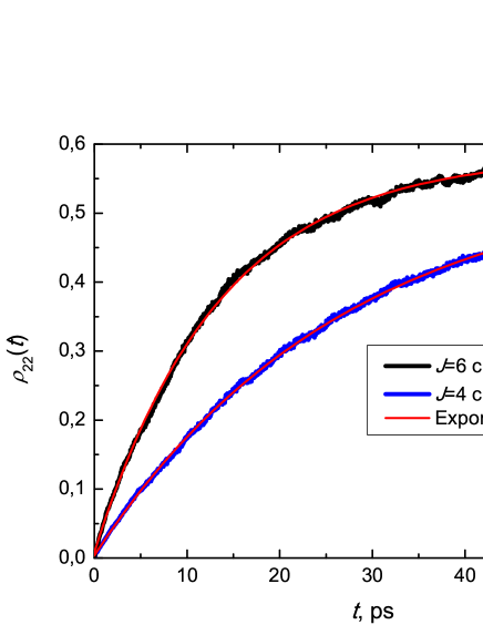
Figure 2: Averaged populations $\rho_{22}(t)$ of two-level systems with different coupling $J$ between the states calculated using Debye spectral density ($\omega_{D}=10\textrm{ fs}^{-1}$, $\lambda=20\textrm{ cm}^{-1}$). Parameters obtained from fitting when $J=4\textrm{ cm}^{-1}$: $A=0.56$, $\tau=27.1\textrm{ ps}$; when $J=6\textrm{ cm}^{-1}$: $A=0.58$, $\tau=13.4\textrm{ ps}$. Averaging is performed over $R=10000$ realizations.

It can be noticed that the populations do not exactly converge to the values defined by the thermal distribution of system states. There are two reasons for this. First, the exact Boltzmann equilibrium values for the populations with respect to the level splittings of 100 cm^-1 can be obtained only when there is no interaction between the system and the bath. Otherwise when system-bath coupling is on, the stationary states become different and the equilibrium values in the simulations are obtained with respect to the full system+bath Hamiltonian. Second, the SSE is nevertheless approximate.

III.2 Excitation transfer time

One of the main characteristic of the energy transfer is the transfer time. This transfer time is the stochastic property, being unique for each member of the ensemblel. Moreover this transfer time is a stochastic property even for a single member of the ensemble. From the theory of stochastic Markovian systems Breuer and Petruccione (2002) it is known that the actual transfer time from the initial state to the final one, when the process is characterized by a single rate constant, must be a random number distributed according to the exponential law with the properly defined mean transfer time, that is the inverse of the rate, i. e. $p(t)=B\exp\left(-k_{1\rightarrow 2}t\right)$. Consequently the mean transfer time is given by $\tau_{1\to 2}=1/k_{1\rightarrow 2}$. Hence, using the FGR (or the Redfield theory), the mean transfer time can be evaluated as the inverse of calculated transfer rates. However, the Redfield theory as well as the rate concepts are valid only for the weak coupling regimes. In the case of intermediate or strong couplings, the HEOM method allows to exactly propagate the density matrix, however, the rates and the transfer times then become undefined. Additional heuristic arguments may be necessary to define the transfer times based on the density matrix population evolutions. We next devise a stochastic method to simulate the excitation transfer time using the SSE, which allows to properly define and evaluate the excitation transfer time distribution function even if it is not exponential.

The meaning of the transfer time implies that we start with the predefined state of the system and after some time we observe another state. Hence, to calculate the transfer time to an arbitrary site of the system, first we have to define the process of the measurement (detection) of the excitation on the necessary site. This measurement procedure can be constructed in the following way. The system wave vector with components $\psi_{n}\left(t\right)$ is a stochastic variable depending on a set of fluctuations $u_{k}\left(t\right)$ according to Eq. (31). Additionally, the magnitudes of the components of the wave vector are generally nonzero. For this reason the system can be found in an arbitrary state at an arbitrary time. We can "measure" the excitation on an arbitrary site of the system by performing the non-destructive quantum measurement of the system state. If the exciton is detected on the $n$-th site, the system state collapses to $\left|n\right\rangle$, we determine the arrival time and stop the propagation because the state before arrival has now collapsed into a new state $\left|n\right\rangle$. The statistical probabilities of these outcomes are $1-\left|\psi_{n}\left(t\right)\right|^{2}$ and $\left|\psi_{n}\left(t\right)\right|^{2}$, respectively. This measurement process can be modeled using the Monte - Carlo method by drawing a random number $r$ uniformly distributed in the interval $[0,1)$ before starting the propagation (1). Now during the propagation as soon as we find $r<\left|\psi_{n}\left(\tau\right)\right|^{2}$, we register the exciton on the $n$-th site and $\tau$ is defined as the transfer time. Due to the fact that the system state evolves stochastically and the random number $r$ takes unique values for each propagation, the exciton detection condition is fulfilled at different time moments in each realization. With a sufficient number of realizations we can then calculate the distribution of the energy transfer time. Hence, the algorithm of the exciton registration at site $n$ and construction of the exciton transfer time distribution can be summarized as follows:

1. A uniformly distributed random number $r$ is generated in the interval $[0,1)$.

2. The system wave vector is propagated, and at every time step the condition $r<\left|\psi_{n}\left(t\right)\right|^{2}$ is checked.

3. If the condition is satisfied, the propagation is stopped and the exciton transfer time to the $n$-th site is recorded; otherwise the propagation (step 2) is being continued.

4. 1-3 stages are repeated for the same system until a statistically sufficient amount of results is obtained.

5. The distribution of transfer times is constructed as the histogram of the arrival times.

This procedure is illustrated in Fig. 1: the exciton detection time is marked by crossing point of $r$ and $|\psi_{2}\left(t\right)|^{2}$. The corresponding distribution of excitation transfer time from site $1$ to $2$ in the weakly-coupled two-site system is presented in Fig. 3 As the FGR holds in this case, we find proper exponential distribution of transfer times. The mean values of the transfer time indeed correspond to the transfer rates, determined from population evolution in Fig. 1.

We must notice that the transfer time distributions in Fig. 3 contain a sharp rise at short times which is not accounted by the probabilistic theory of Markovian processes. This rise is the result of transient processes caused by slight non-Markovianity of the bath at short times originating from the finite-time correlation function for the environmental fluctuations. In our case the correlation time of the environment fluctuations is 10 fs. This initial rise corresponds to this time. In the ideal Markovian case the fluctuation would be infinitely fast (white noise) and the initial rise and transition into the exponential function would happen at infinitesimal time interval.

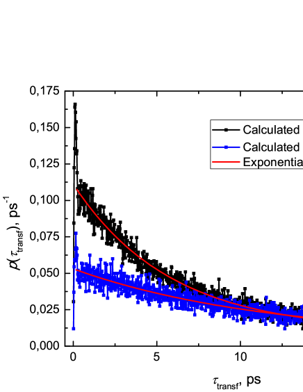
Figure 3: Probability density functions of the transfer time $\tau_{\textrm{transf}}$ from the initially occupied state to the unoccupied state in two-level systems with different coupling $J$ between the states calculated using Debye spectral density ($\omega_{D}=10\textrm{ fs}^{-1}$, $\lambda=20\textrm{ cm}^{-1}$). Parameters obtained from fitting when $J=4\textrm{ cm}^{-1}$: $B=8.4\cdot 10^{-5}$, $\tau_{1\to 2}=11.1\textrm{ ps}$; when $J=6\textrm{ cm}^{-1}$: $B=1.3\cdot 10^{-4}$, $\tau_{1\to 2}=5.7\textrm{ ps}$.

III.3 Relaxation in a strongly-coupled model system

We next consider the intermediate-to-strong coupling regime. Again we study the two-site system, but we choose model parameters for intermediate couplings consistent with ref. Ishizaki et al. (2010) : $\varepsilon_{1}=100\textrm{ cm}^{-1}$, $\varepsilon_{2}=0\textrm{ cm}^{-1}$, $J_{12}=J_{21}=100\textrm{ cm}^{-1}$. For the environment we choose the Debye spectral density (the same for the both sites), with $\lambda=100\textrm{ cm}^{-1}$ and $\omega_{\textrm{D}}=100\textrm{ fs}^{-1}$ and study relaxation at two temperatures. The initial condition is $|\psi\left(0\right)\rangle=\sum_{n}\delta_{n1}|n\rangle$. The population of the second site is presented in Fig. 4. We can see that at both heat bath temperatures ($T=300\textrm{ K}$ and $T=77\textrm{ K}$) the population rises very quickly in the first 100 fs and then performs oscillatory motion until it reaches the equilibrium value. It should be noted that in case of higher environmental temperature the amplitude of the population oscillations is smaller and they are damped quicker ($\sim 300\textrm{ fs}$) than in the case of low temperature when oscillations die out after $\sim 500\textrm{ fs}$. The oscillations are mostly Rabi beats due to coupling $J$ and nonstationary initial state. The damping is due to the bath. It has been discussed that the approximate Redfield theory is not appropriate for this system, since the relaxation rates and consequently the excitation transfer times can not be accurately defined Gelzinis et al. (2011). For comparison we also present the density matrix propagation results using the Redfield theory with the time-dependent relaxation kernel (Eq. 30). The Redfield theory result shows large deviations from the SSE result. However, as both are approximate, the provided information is not sufficient to judge about correctness. Therefore we additionally present the dependencies calculated using the exact HEOM method. We can see that both methods give results that coincide perfectly at the beginning of the simulation. We can also notice that the equilibrium values of the populations calculated with the SSE agree well with those obtained with the HEOM method and this correspondence is better the higher is the temperature of the environment. It is evident that the Redfield method gives largest errors. At low temperatures some deviations between HEOM and SSE are moderate, however the results of the stochastic method qualitatively reproduce the character of the HEOM dependencies from short to intermediate times when transient processes are present in the system.

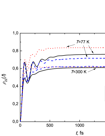
Figure 4: Time dependencies of the population $\rho_{22}\left(t\right)$ at different bath temperatures calculated using SSE, Redfield and HEOM methods. For SSE averaging is performed over $R=10000$ realizations.

The dynamics of the two-site system with the above-given parameters and heat bath characteristics should be rather non-Markovian due to the long decay time of the bath correlation function (100 fs) and this behavior must be reflected in the distributions of the exciton transfer time. These distributions are presented in Fig. 5. Comparing these results with distributions obtained for the weakly interacting Markovian system (Fig. 3) we clearly see that now the distributions are not exponential which indicates the significance of non-Markovian effects in this two-site system. The second peak in the transfer time signifies the coherent components. We can notice that the duration of the initial rise of the probability density functions corresponds to the relaxation time of the heat bath ($\omega_{\textrm{D}}=100\textrm{ fs}^{-1}$). Such non-exponential distributions do not correspond to any process described by simple constant-rate equations, which define the transfer mean times. Thus, in this respect the SSE approach has an advantage in describing energy transfer over the density matrix approaches.

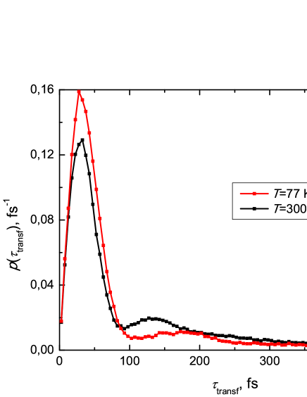
Figure 5: Probability density functions of the transfer time $\tau_{\textrm{transf}}$ from the initially occupied state to the unoccupied state in the two-level system at different bath temperatures calculated using Debye spectral density ($\omega_{\textrm{D}}=100\textrm{ fs}^{-1}$, $\lambda=100\textrm{ cm}^{-1}$).

IV Case study: Exciton dynamics in the FMO complex

FMO complex found in the green sulfur bacteria is the first pigment - protein which had its structure revealed using the method of X-ray crystallography, hence it is one of the best studied photosynthetic aggregates Engel et al. (2007); Mohseni et al. (2008); Panitchayangkoon et al. (2010); Milder et al. (2010). FMO complex is a trimer consisting of 3 identical monomers which are formed from 8 bacteriochlorophyll (BChl) molecules supported by a rigid protein carcass (Fig. 6). In green sulfur bacteria the FMO aggregate acts as a molecular wire which transports the excitation energy from the light-harvesting chlorosomes to the reaction centers of the I type located in the membrane Engel et al. (2007); Mohseni et al. (2008); Panitchayangkoon et al. (2010). We next apply the the SSE theory and the simulation protocol described above to study the energy transfer dynamics in the FMO aggregate.

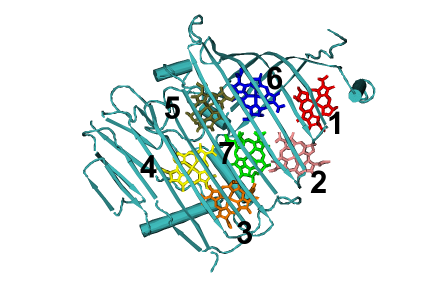
Figure 6: Arrangement of the bacteriochlorophylls in one monomer of the FMO complex.

The FMO complex is described by the Hamiltonian adapted from previous publications Mohseni et al. (2008). We assume that the FMO system consists only of 7 sites corresponding to different BChl molecules. The 8th molecule is not taken into account due to its weak coupling with the rest of the BChls. Setting the energy of the 3rd site, through which the energy excitation travels to the reaction center, to zero, we obtain the matrix:

	1.	2.	3.	4.	5.	6.	7.
1.	280	-106	0	0	0	-8	-4
2.		420	28	0	0	13	0
3.			0	-62	0	0	17
4.				175	-70	-19	-57
5.					320	40	-2
6.						360	32
7.							260

Table 1: Matrix elements of the FMO Hamiltonian given in $\textrm{cm}^{-1}$. Sites are numbered according to the crystallographic nomenclature Fenna et al. (1977).

In all simulations of the FMO system the initial state was chosen to be a superposition $\left|\psi\left(0\right)\right\rangle=\frac{1}{\sqrt{2}}\left(\left|1\right\rangle+\left|6\right\rangle\right)$. This state is chosen because the 1st and the 6th BChl molecules are nearest to the light-harvesting chlorosomes where the excitation is created Mohseni et al. (2008). The interaction with the environment induces fluctuations of the excitation energies of the BChl molecules. Classical correlation functions of these energy fluctuations for every BChl molecule have been estimated by the Olbrich et al molecular dynamics (MD) simulations of the whole FMO complex in the solution Olbrich et al. (2011). These correlation functions have been approximated by a combination of exponents and decaying oscillations. After performing the Fourier transformation the spectral densities of different BChl molecules at room temperature ($T=300$ K) have been obtained:

$$C_{\textrm{MD},n}^{\prime\prime}\left(\omega\right)=\frac{2}{\pi\hbar}\tanh\left(\frac{\beta_{T}\hbar\omega}{2}\right)\left[\overset{N_{0}}{\underset{m=1}{\sum}}\frac{\eta_{n,m}\gamma_{n,m}}{\gamma_{n,m}^{2}+\omega^{2}}\right.$$

$$\hskip 10.03749pt\hskip 8.03pt\hskip 30.11249pt\left.+\overset{N_{0}}{\underset{m=1}{\sum}}\frac{\widetilde{\eta}_{n,m}\widetilde{\gamma}_{n,m}}{2\left(\widetilde{\gamma}_{n,m}^{2}+\left(\omega-\widetilde{\omega}_{n,m}\right)^{2}\right)}\right].$$

(42)

$\eta_{n}$, $\gamma_{n}$, $\widetilde{\eta}_{n}$ and $\widetilde{\omega}_{n}$ are parameters best fitting the corresponding correlation functions and $N_{0}$ is the number of terms in the sum. In this expression the factor $\tanh\left(\frac{\beta_{T}\hbar\omega}{2}\right)$ is introduced to take into account the temperature dependence of the parameters. In the following we denote this spectral density as the MD spectral density.

The spectral density given above consists mainly of two terms. The first is a Debye term determining the overdamped low frequency modes. The second part reflects the high-frequency modes. These should be associated with the intra-molecular vibrations. As the intra-molecular vibrational frequencies are the same for all chrolophylls, while their amplitudes vary from site to site, for simplicity we assume the averaged spectral density for all BChl molecules with $N_{0}=12$ terms in Eq. (42). As a reference, a model without high frequency intra-molecular vibrations based on the Debye spectral density (Eq. (36)) is used as well. Both Debye and MD spectral densities have similar low-frequency part, while they are different at high frequencies as shown in Fig. 7. The low frequency part also corresponds to the experimentally determined spectral density Wendling et al. (2000) in this range of frequencies.

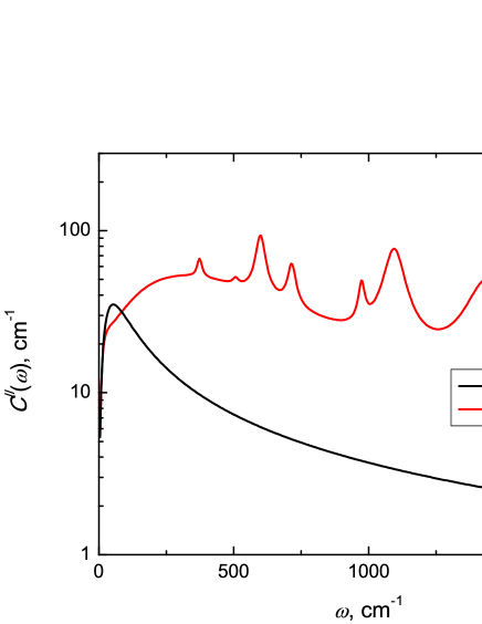
Figure 7: Debye and MD spectral densities used for FMO complex. Parameters of Debye spectral density: $\omega_{D}=100\textrm{ fs}^{-1}$, $\lambda=35\textrm{ cm}^{-1}$ were set according to Ref. Ishizaki and Fleming (2009c).

The dynamics and relaxation of the excitation in the aggregate can be investigated by first analyzing time dependencies of the site populations. These, averaged over the ensemble according to Eq. 41 at the temperature $T=300$, are presented in Fig. 8. We can see from both figures that when the system approaches equilibrium the value of the population $\rho_{33}\left(t\right)$, which corresponds to the site with the lowest energy $\varepsilon_{3}=0$, becomes the largest in accord with previous simulations Nalbach and Thorwart (2012). Equilibrium values of populations of other sites are also ordered in accord with their energy corresponding to proper thermal equilibrium. Time dependencies of the populations calculated with Debye spectral density (Fig. 8 (a)) show that despite of populations $\rho_{44}\left(t\right)$, $\rho_{55}\left(t\right)$, $\rho_{66}\left(t\right)$ and $\rho_{77}\left(t\right)$ reaching equilibrium after $\sim 2\textrm{ ps}$, other curves are still not stationary, thus the full relaxation of the system occurs in more than 5 ps. The results obtained with MD spectral density are depicted in Fig. 8 (b) demonstrate qualitatively similar but slightly quicker relaxation process. The coherent evolution as well as delocalized excitons in the system can be recognized from the oscillations of the presented populations. From the calculations with Debye spectral density we can see that oscillations decay after $\sim 500\textrm{ fs}$. Using MD spectral density we obtain smaller amplitudes of oscillations and they decay faster - after $\sim 300\textrm{ fs}$. That manifests the decay of electronic coherences. Hence the MD spectral density seems to slightly speed-up the relaxation dynamics without noticeable qualitative differences.

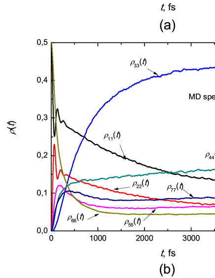
Figure 8: System population dependencies on time calculated in the site basis: (a) with Debye spectral density ($\omega_{\textrm{D}}=100\textrm{ fs}^{-1}$, $\lambda=35\textrm{ cm}^{-1}$), (b) with MD spectral density. Averaging is performed over $R=10000$ realizations.

The most important result of this study which is available from the SSE is the distribution of excitation transfer times. These distributions for all seven sites calculated at temperature $T=300$ K are presented in Fig. 9. It is evident that all distributions calculated with both spectral densities greatly differ from the exponential form. We can notice that with both spectral densities result in similar overall arrangement of the exciton transfer time distribution curves and also the most probable transfer times. It is evident that the energy excitation can be registered at the 1st or the 6th site in the shortest time. Analyzing the positions of the maxima of the probability distributions we can see that the exciton travels through the FMO complex in such order: 2nd site, 5th site, 7th site, 4th site and it takes the longest time for the exciton to arrive at the 3rd site. Hence, the transfer time distributions reveal the excitation transfer pathways in multi-site excitonic systems. From the Fig. 9 we can also see that the transfer time distribution at the 3rd site is the broadest, which means that in this case the time $\tau_{\textrm{transf}}$ has the biggest uncertainty.

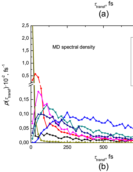
Figure 9: Distributions of energy excitation transfer time calculated for all sites of the system: (a) with Debye spectral density ($\omega_{\textrm{D}}=100\textrm{ fs}^{-1}$, $\lambda=35\textrm{ cm}^{-1}$), (b) with MD spectral density.

V Discussion

In this paper we employ the SSE to study relaxation of molecular excitations where the system state is described by the stochastic vector $\left|\psi\left(t\right)\right\rangle$. While the mathematical formulation of the problem is transparent, the physical meaning of stochastic quantities requires additional discussion. The origin of the stochasticity of $|\psi(t)\rangle$ vector stems from the fact that the environmental quantum variables, $\bm{\alpha}$ and $\bm{\beta}$, are interpreted as complex-valued Gaussian fluctuations acting on our investigated system. This step introduces the ambiguity in interpretation of the stochastic vector $|\psi(t)\rangle\equiv\left|\psi\bm{\alpha}_{\phi\bm{\beta}}\left(t\right)\right\rangle$.

One’s initial guess might be that the wavevector describes the state of the reduced system $\psi$ at an arbitrary time. This initial guess contains a flaw since based on the quantum mechanics the system and bath parts inevitably must be entangled as time passes and the "reduced wavefunction of the system" does not exist. The state of the composite system+bath system must be understood as a linear superposition in the basis of composite system+bath vectors $|n\bm{\alpha}\rangle$:

$$|\Psi\rangle=\sum_{n}\int\frac{\mathrm{d}\bm{\alpha}}{\pi}c_{n\bm{\alpha}}(t)|n\bm{\alpha}\rangle;$$ (43)

$n$ is taken as a discrete variable and $\bm{\alpha}$ is a continuous, while $c_{n\bm{\alpha}}(t)$ is the specific component with respect to the basis. What does $\left|\psi\bm{\alpha}_{\phi\bm{\beta}}\left(t\right)\right\rangle$ stand for? Let us remind that this quantity was obtained by taking the factorized initial condition $\left|\phi\bm{\beta}\right\rangle$, which properly denotes the initial state. The state is then propagated for a time $t$ by an evolution operator. $\left|\psi\bm{\alpha}_{\phi\bm{\beta}}\left(t\right)\right\rangle$ is thus a specific $\bm{\alpha}$ component of the complete wavefunction with respect to the initial condition $\left|\phi\bm{\beta}\right\rangle$. This component becomes available by collapsing the environment wavefunction into the $|\bm{\alpha}\rangle$ state or in other words by measurement of the $|\bm{\alpha}\rangle$ state. Probability of such collapse, which should be realized by a quantum measurement, is given by the norm of the vector $\left|\psi\bm{\alpha}_{\phi\bm{\beta}}\left(t\right)\right\rangle$. Hence, the SSE describes a single $\bm{\alpha}$ component of the full wavefunction. So how about other components and where does the stochasticity comes from? This is an additional ingredient in the stochastic equation, which takes into account the probability density (Eq. (17)). Notice that the complete specification of vectors $\bm{\alpha}$ and $\bm{\beta}$ completely determines functions $z_{n}(t)$ and $w_{n}(t)$. These functions are merely kind-of Heisenberg representation of $\bm{\alpha}$ and $\bm{\beta}$. So when the component of the complete wavefunction is chosen, the whole "trajectories" $z_{n}(t)$ and $w_{n}(t)$ are specified and stochasticity is removed. The different component is obtained by taking $\bm{\alpha}^{\prime}\neq\bm{\alpha}$, hence, by taking another function $z_{n}^{\prime}(t)$ corresponding to $\bm{\alpha}^{\prime}$. Smart way of choosing set of different $\bm{\alpha}$s (or $u_{n}(t)$ as described in Sec. II.2) guarantees proper probability distribution of different trajectories. Consequently the whole wavefunction of the composite system is calculated by combining the ensemble of functions $z_{n}(t)$ reflecting all possible realizations of vector $\bm{\alpha}$. In this sense the whole procedure of averaging over various trajectories becomes similar to the path-integral formulation. The paths are distributed non-uniformly, but follow the Gaussian distribution.

Now the natural question is whether some interpretation of a single $z(t)$ and $w(t)$ trajectory is possible? We would like to argue that yes it is. Recall that a vector characterizing the system of interest alone can be defined if we measure the state of the environment. Thus, after performing this measurement at $\bm{\alpha}$ the full wavefunction of the composite system becomes a tensor product - $\left|\Psi\right\rangle=|\psi\bm{\alpha}\rangle$. The probabilities of the site populations should be understood also conditioned on the state $\bm{\alpha}$. These conditional probabilities thus reflect the renormalization procedure, which we implied before. The $|\psi\bm{\alpha}\rangle$ vector is then the system wave vector conditioned on the result of the measurement of the environment state at $\bm{\alpha}$ (also, provided the initial state was $\bm{\beta}$). According to the SSE (Eq. (28)) the $\kappa^{1}$ term induces the fluctuations of the Hamiltonian elements. Hence, a single configuration of the bath $(\bm{\alpha},\bm{\beta})$ defines the full trajectory of the fluctuating Hamiltonian, or the effect of the bath configuration $(\bm{\alpha},\bm{\beta})$ on the whole time interval through functions $z(t)$ and $w(t)$. As the bath configuration has the probability $\exp\left(-|\alpha|^{2}-|\beta|^{2}\textrm{e}^{\beta_{T}\omega_{j}}+2\Re(\alpha^{*}\beta)\right)$, the fluctuating trajectory of the Hamiltonian has the same probability. With this in mind, we can interpret the single trajectory as the action of the environment (being in state $\bm{\alpha}$) on the system through $z(t)$ (and $w(t)$) continuously. Hence, the state of the bath, defined by $\bm{\alpha}$ (and $\bm{\beta}$) defines the whole time trajectory. This phenomenon reflects the concept of non-locality of quantum mechanics.

It should be denoted that the interpretation described in the previous paragraph gives a false impression as if the bath does not respond to the system dynamics. This indeed follows from $\kappa^{1}$ approach as the Hamiltonian is linear to Gaussian fluctuations $z(t)$ and $w(t)$. The picture is slightly different as we consider terms $\kappa^{2}$ or higher (Eq. (28)). With $\kappa^{2}$ terms the time-dependent Hamiltonian is also affected by the correlation function of the fluctuations, hence the relaxation of the bath with respect to system state is then included up to $\kappa^{2}$. The $\kappa^{2}$ terms, hence, reflect the back-action, which becomes non-local and contains the memory of the action. The higher orders of the action by environment could be included by expanding the non-local exponential function in Eq. (28).

These properties ensure that the dynamics of a composite system+environment system is treated in the correlated fashion, i. e., the system is affected by the environment and the environment is affected by the the system dynamics. These properties allow to describe correlated dissipative properties, such as for instance polaronic effects, which appear to be quite important for molecular excitations. The polaron formation effect has been captured from the equilibrium density matrix using the HEOM Gelzinis et al. (2011). The effective resonant coupling has been found to depend exponentially on the system-bath coupling strength. The time evolution of this relaxation has been revealed using the variational approach Chorosajev et al. (2013) and various polaron formation scenarios have been obtained. The SSE could be used to reveal the dynamical Hamiltonian as well, thus these effects are captured in the excitation dynamics presented in this paper. Additionally the SSE includes the coherent effects such as high-frequency molecular vibrations through resonances of the spectral densities. While the spectral density approach has limitations in the exciton basis (which must be fluctuating due to bath dynamics and the cumulant expansion is not valid), we avoid problems as we treat the problem in the site basis, which is independent of the fluctuations. Hence the resonances of the spectral density, reflecting the intra-molecular vibrations are properly included.

The exact treatment of the open quantum system dynamics at the level of HEOM requires solving the general form of the SSE (Eq. (28)). However, we have showed that time-local SSE (Eq. 31), obtained by making second order to the system-bath interaction approximation guarantees quite accurate results at room temperature. Additionally, possibility to renormalize the wave-function at an arbitrary time allows to avoid problems of divergencies. Consequently we can see from Fig. 4 that the SSE performs considerably better than the Redfield equation, especially at low temperatures. Another useful property of the SSE method is that it does not impose any restrictions on the spectral density of the heat bath - according to Eq.(40) fluctuations $u_{n}\left(t\right)$ can be generated with the function $C^{\prime\prime}\left(\omega\right)$ of arbitrary form and, thus, describe various environments of the system, including the high-frequency intra-molecular vibrations.

The theory of decoherence Schlosshauer (2007) dictates that the interaction between the system an environment (effectively the measurement) causes decoherence in the system and final collapse of the system state into the so-called preferred state which is uniquely defined by the "measurement device". In this interpretation the dynamics of the open quantum system can be understood in terms of the continous measurement which damps the system dynamics. Such approach has been successfully used in describing the quantum dynamics Bittner and Rossky (1995, 1997); Bittner et al. (1997). We use the concept of measurement at few points as well. First, our simulation trajectory corresponds to the measurement of the state of the bath $|\bm{\alpha}\rangle$. Second, we perform measurement of the excitation position when we define the transfer time. Compared to result of Refs. Bittner and Rossky (1995, 1997); Bittner et al. (1997) the whole ensemble of our trajectories then correspond to decoherence of system wavevector as the wavevector diverges for different bath trajectories (see Fig. 1).

The stochastic nature of the wave vector enables us to calculate the stochastic properties of the system and this feature is a big advantage of the SSE formalism over the reduced density matrix methods. One of the important properties available from the SSE is the exciton transfer time distribution. The stochastic transfer times of the exciton and their distribution are proper quantities in our approach, while the reduced density matrix formalism do not define them when the processes are non-exponential. Our procedure of obtaining the stochastic transfer time from the SSE is based on an assumption of a quantum measurement of the system state with the $N$-slit-like measurement device in analogy with the two-slit experiment: the stochastic populations of the system represent the probabilities to find the exciton on a particular site and the random number $r$ models the operation of the exciton detector at one of the “slits” Schlosshauer (2007). The adequacy of this procedure of exciton transfer time calculation has been illustrated by applying this method to a two level system interacting with a nearly Markovian heat bath which means that the environmental processes are much faster than those in the system. For a two-level system the waiting time coincides with our definition of the transfer time.

The two-site model system presented in this paper allows to validate various angles of our approach: in the Markovian weak-coupling case we find all necessary properties of the dynamics consistent with the theoretical predictions including the proper thermal equilibrium, correct scaling of transfer rates, as well as proper exponential distributions of transfer times. The strong-coupling case has non-exponential evolutions, consistent with exact HEOM approach.

However, the main result obtained in this paper is the conclusion on the effect of intra-molecular high-frequency vibrations on the energy transfer dynamics in photosynthetic FMO aggregate. Recent 2D spectroscopy experiments revealed long-lasting quantum coherences in FMO and a range of other systems Lee et al. (2007); Pachón and Brumer (2011); Schlau-Cohen et al. (2012). There is a continuous debate on the origin of these beats, while their assignment recently was shifted to be vibrational. The role of the coherence is considered to be an important factor for defining the excitation dynamics in molecular aggregates. We hence addressed the very core of the problem and simulated the excitation transfer processes by including or excluding the high-frequency vibrations. As revealed by the exciton transfer time distribution to the 3rd FMO site shown in Fig. 10, the overall dynamics certainly becomes slightly faster, however, the excitation transfer pathways are not very sensitive to the choice of the spectral density, i. e., whether we have or do not have high frequency vibrational modes. It could be argued that the system-bath coupling strength parameters, the reorganization energies, of both spectral densities are different so the results are hardly comarable. However, the reorganization energy, includes contributions from both the low frequency and the high frequency components, so obviously the two models of spectral density cannot have the same reorganization energy. However, the low frequency pars of the spectral densities are comparable, so the effect on the transfer times is necesseraly related to the high frequency spectral components.

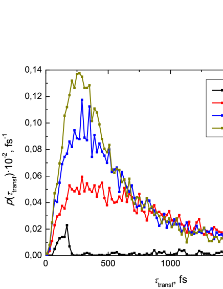
Figure 10: Distributions of energy excitation transfer time calculated for the 3rd site in the FMO system at different system - bath interaction strengths. Debye frequency $\omega_{\textrm{D}}=100\textrm{ fs}^{-1}$, $T=300\textrm{ K}$.

Appendix A Some properties of coherent state representation

The coherent state $\left|\alpha\right\rangle$ is defined as the eigenvector of the annihilation operator $\widehat{a}$:

$$\widehat{a}\left|\alpha\right\rangle=\alpha\left|\alpha\right\rangle.$$ (44)

The annihilation operator is not Hermitian, thus the quantity $\alpha$ in Eq. (44) is a complex number and can get any value. The representation of the coherent state $\left|\alpha\right\rangle$ in the energy eigenbasis of the harmonic oscillator $\left|n\right\rangle$ can be obtained by calculating the scalar product of both sides of Eq. (44) with the vector $\left\langle n\right|$ which yields

$$\left|\alpha\right\rangle=C\overset{\infty}{\underset{n=0}{\sum}}\frac{\alpha^{n}}{\sqrt{n!}}\left|n\right\rangle.$$ (45)

Choosing $C$ to be equal to 1 we can calculate using Eq. (45) the scalar product of two coherent states $\left\langle\alpha\right|$ and $\left|\beta\right\rangle$

$$\left\langle\alpha|\beta\right\rangle=\textrm{e}^{\alpha^{*}\beta}.$$ (46)

From Eq. (46) we can see that the coherent states $\left|\alpha\right\rangle$ are not normalized because $\left\langle\alpha|\alpha\right\rangle=\textrm{e}^{|\alpha|^{2}}\neq 1$. Despite the fact that the coherent states $\left|\alpha\right\rangle$ being the eigenvectors of a non-Hermitian operator $\widehat{a}$ are not orthogonal, they still can be used to construct the identity operator

$$\widehat{\boldsymbol{1}}=\int\frac{\textrm{d}^{2}\alpha}{\pi}\textrm{e}^{-|\alpha|^{2}}\left|\alpha\right\rangle\left\langle\alpha\right|,$$

where $\textrm{d}^{2}\alpha\equiv\textrm{d}\left[\textrm{Re}\alpha\right]\textrm{d}\left[\textrm{Im}\alpha\right]$ and the factor $\textrm{e}^{-|\alpha|^{2}}$ ensures the proper normalization Gazeau (2009).

Another useful property of the coherent states can be obtained by noticing that the vector $\left\langle\alpha\right|\widehat{a}$ can be written as $\frac{\partial}{\partial\alpha^{*}}\left\langle\alpha\right|$:

$$\left\langle\alpha\right|\widehat{a}=\overset{\infty}{\underset{n=0}{\sum}}\frac{\left(\alpha^{*}\right)^{n}}{\sqrt{n!}}\left\langle n\right|\widehat{a}$$

$$=\overset{\infty}{\underset{n=0}{\sum}}\frac{\left(n+1\right)\left(\alpha^{*}\right)^{n}}{\sqrt{\left(n+1\right)!}}\left\langle n+1\right|=\frac{\partial}{\partial\alpha^{*}}\left\langle\alpha\right|.$$

(47)

Using this property we can deal with the problem of extraction of the system wave vector from the third term in Eq. (22):

$$\textrm{e}^{-\alpha^{*}\beta}\left\langle\boldsymbol{\alpha}\right|\widehat{U}\left(t-\tau\right)\widehat{L}_{m}\widehat{U}^{\dagger}\left(t-\tau\right)\widehat{U}\left(t\right)\left|\boldsymbol{\beta}\right\rangle\left|\phi\right\rangle$$

$$=\hat{T}\textrm{e}^{-i\overset{t}{\underset{\tau}{\int}}\textrm{d}\tau^{\prime}\widehat{\mathcal{H}}_{\alpha}\left(\tau^{\prime}\right)}\widehat{L}_{m}\hat{T}\textrm{e}^{i\overset{t}{\underset{\tau}{\int}}\textrm{d}\tau^{\prime}\widehat{\mathcal{H}}_{\alpha}\left(\tau^{\prime}\right)}\left|\psi\bm{\alpha}_{\phi\bm{\beta}}\left(t\right)\right\rangle.$$

(48)

Here we used the expression of the evolution operator $\widehat{U}\left(t\right)=\hat{T}\textrm{e}^{-i\overset{t}{\underset{0}{\int}}\textrm{d}\tau^{\prime}\widehat{H}\left(\tau^{\prime}\right)}$ in the interaction representation, which involves the time-ordering operator $\hat{T}$ and e denotes the exponential series. The operator in the exponent is

$$\widehat{\mathcal{H}}_{\bm{\alpha}}\left(t\right)=\widehat{H}_{S}$$

$$+\kappa\underset{n}{\sum}\underset{j}{\sum}\left[\widehat{L}_{n}g_{nj}\textrm{e}^{i\omega_{j}t}\alpha_{j}^{*}+\widehat{L}_{n}^{\dagger}g_{nj}^{*}\textrm{e}^{-i\omega_{j}t}\frac{\partial}{\partial\alpha_{j}^{*}}\right].$$

(49)

Also we introduce a new operator $\widehat{A}_{\bm{\alpha}}\left(t-\tau\right)$:

$$\widehat{A}_{\bm{\alpha}}\left(t-\tau\right)=\hat{T}\textrm{e}^{-i\overset{t}{\underset{\tau}{\int}}\textrm{d}\tau^{\prime}\widehat{\mathcal{H}}_{\alpha}\left(\tau^{\prime}\right)}.$$ (50)

This expression is used in Eq. (28).

Appendix B Equilibrium density operator in the coherent state representation

It can be shown that every operator $\widehat{O}$ which has square integrable matrix elements $\left\langle-\alpha\left|\widehat{O}\right|\alpha\right\rangle$ can be expressed in the coherent state basis as a diagonal operator Mehta (1967):

$$\widehat{O}=\int\frac{\textrm{d}^{2}\beta}{\pi}\varphi(\beta)\left|\beta\right\rangle\left\langle\beta\right|,$$ (51)

where the function $\varphi(\beta)$ is equal to

$$\varphi(\beta)=\int\frac{\textrm{d}^{2}\alpha}{\pi}\left\langle-\alpha\left|\widehat{O}\right|\alpha\right\rangle\textrm{e}^{\beta\alpha^{*}-\beta^{*}\alpha}.$$ (52)

Both expressions (51) and (52) are also valid in the multidimensional case with $\left|\boldsymbol{\alpha}\right\rangle$ and $\left|\boldsymbol{\beta}\right\rangle$.

To calculate the bath equilibrium density operator $\widehat{\rho}_{B}$ in the coherent state basis we must first calculate the matrix element $\left\langle-\boldsymbol{\alpha}\left|\widehat{\rho}_{B}\right|\boldsymbol{\alpha}\right\rangle$:

$$\left\langle-\boldsymbol{\alpha}\left|\widehat{\rho}_{B}\right|\boldsymbol{\alpha}\right\rangle=Z^{-1}\left\langle-\boldsymbol{\alpha}\left|\textrm{e}^{-\beta_{T}\widehat{H}_{B}}\right|\boldsymbol{\alpha}\right\rangle$$

$$=\overset{\infty}{\underset{j=1}{\prod}}\frac{1}{\overline{n}_{j}+1}\exp\left(-|\alpha_{j}|^{2}\textrm{e}^{-\beta_{T}\omega_{j}}\right).$$ (53)

where $\overline{n}_{j}=\left(\textrm{e}^{\omega_{j}\beta_{T}}-1\right)^{-1}$ is the Bose - Einstein function. Now the function $\varphi(\boldsymbol{\beta})$:

$$\varphi(\boldsymbol{\beta})=\int\frac{\textrm{d}^{2}\boldsymbol{\alpha}}{\pi}\left\langle-\boldsymbol{\alpha}\left|\widehat{\rho}_{T}\right|\boldsymbol{\alpha}\right\rangle\textrm{e}^{\beta\alpha^{*}-\beta^{*}\alpha}$$

$$=\overset{\infty}{\underset{j=1}{\prod}}\frac{1}{\overline{n}_{j}}\exp\left(-|\beta_{j}|^{2}\textrm{e}^{\beta_{T}\omega_{j}}\right).$$ (54)

Finally, using the expression (54) and according to Eq. (51) we can write the equilibrium density operator of the heat bath

$$\widehat{\rho}_{T}=\overset{\infty}{\underset{j=1}{\prod}}\int\frac{\textrm{d}^{2}\beta_{j}}{\pi}\frac{1}{\overline{n}_{j}}\exp\left(-|\beta_{j}|^{2}\textrm{e}^{\beta_{T}\omega_{j}}\right)\left|\beta_{j}\right\rangle\left\langle\beta_{j}\right|.$$ (55)

References

- Engel et al. (2007) G. S. Engel, T. R. Calhoun, E. L. Read, T.-K. Ahn, T. Mančal, Y.-C. Cheng, R. E. Blankenship, and G. R. Fleming, Nature 446, 782 (2007).
- Panitchayangkoon et al. (2010) G. Panitchayangkoon, D. Hayes, K. A. Fransted, J. R. Caram, E. Harel, J. Wen, R. E. Blankenship, and G. S. Engel, Proc. Natl. Acad. Sci. U.S.A. 107, 12766 (2010).
- Novoderezhkin and van Grondelle (2010) V. I. Novoderezhkin and R. van Grondelle, Phys. Chem. Chem. Phys. 12, 7352 (2010).
- Ishizaki et al. (2010) A. Ishizaki, T. R. Calhoun, G. S. Schlau-Cohen, and G. R. Fleming, Phys. Chem. Chem. Phys. 12, 7319 (2010).
- Olaya-Castro and Scholes (2011) A. Olaya-Castro and G. D. Scholes, Int. Rev. Phys. Chem. 30, 49 (2011).
- Mennucci and Curutchet (2011) B. Mennucci and C. Curutchet, Phys. Chem. Chem. Phys. 13, 11538 (2011).
- Schlau-Cohen et al. (2011) G. S. Schlau-Cohen, A. Ishizaki, and G. R. Fleming, Chem. Phys. 386, 1 (2011).
- König and Neugebauer (2012) C. König and J. Neugebauer, ChemPhysChem 13, 386 (2012).
- Pachón and Brumer (2011) L. A. Pachón and P. Brumer, J. Phys. Chem. Lett. 2, 2728 (2011).
- Cheng and Fleming (2009) Y.-C. Cheng and G. R. Fleming, Annu. Rev. Phys. Chem. 60, 241 (2009).
- Mančal et al. (2012) T. Mančal, N. Christensson, V. Lukeš, F. Milota, O. Bixner, H. F. Kauffmann, and J. Hauer, J. Phys. Chem. Lett. 3, 1497 (2012).
- Christensson et al. (2012) N. Christensson, H. F. Kauffmann, T. Pullerits, and T. Mančal, J. Phys. Chem. B 116, 7449 (2012).
- Mančal et al. (2010) T. Mančal, A. Nemeth, F. Milota, V. Lukeš, H. F. Kauffmann, and J. Sperling, J. Chem. Phys. 132, 184515 (2010).
- Chachisvilis et al. (1995) M. Chachisvilis, H. Fidder, T. Pullerits, and V. Sundström, J. Raman Spectrosc. 26, 513 (1995).
- Milder et al. (2010) M. T. Milder, B. Brüggemann, R. van Grondelle, and J. L. Herek, Photosynth. Res. 104, 257 (2010).
- Kreisbeck et al. (2013) C. Kreisbeck, T. Kramer, and A. Aspuru-Guzik, J. Phys. Chem. B 117, 9380 (2013).
- Butkus et al. (2012) V. Butkus, D. Zigmantas, L. Valkunas, and D. Abramavicius, Chem. Phys. Lett. 545, 40 (2012).
- Butkus et al. (2013) V. Butkus, D. Zigmantas, D. Abramavicius, and L. Valkunas, Chem. Phys. Lett. 587, 93 (2013).
- Westenhoff et al. (2012) S. Westenhoff, D. Paleček, P. Edlund, P. Smith, and D. Zigmantas, J. Am. Chem. Soc. 134, 16484 (2012).
- Valkunas et al. (2013) L. Valkunas, D. Abramavicius, and T. Mančal, Molecular Excitation Dynamics and Relaxation: Quantum Theory and Spectroscopy (John Wiley & Sons, 2013).
- Breuer and Petruccione (2002) H. P. Breuer and F. Petruccione, The theory of open quantum systems (Oxford university press, 2002).
- May and Kühn (2004) V. May and O. Kühn, Charge and Energy Transfer Dynamics in Molecular Systems (Wiley-VCH, 2004).
- Hashitsume et al. (1992) N. Hashitsume, M. Toda, R. Kubo, and N. Saitō, Statistical physics II: nonequilibrium statistical mechanics (Springer, 1992).
- Redfield (1957) A. G. Redfield, IBM J. Res. Dev. 1, 19 (1957).
- Lindblad (1976) G. Lindblad, Commun. Math. Phys. 48, 119 (1976).
- Gorini et al. (1978) V. Gorini, A. Frigerio, M. Verri, A. Kossakowski, and E. Sudarshan, Rep. Math. Phys. 13, 149 (1978).
- Abramavicius and Mukamel (2010) D. Abramavicius and S. Mukamel, J. Chem. Phys. 133, 064510 (2010).
- Prior et al. (2010) J. Prior, A. W. Chin, S. F. Huelga, and M. B. Plenio, Phys. Rev. Lett. 105, 050404 (2010).
- Chin et al. (2011) A. W. Chin, S. F. Huelga, and M. B. Plenio, Quantum Efficiency in Complex Systems, Part II: From Molecular Aggregates to Organic Solar Cells: Organic Solar Cells 85, 115 (2011).
- Tanimura (2006) Y. Tanimura, J. Phys. Soc. Jpn. 75, 082001 (2006).
- Ishizaki and Fleming (2009a) A. Ishizaki and G. R. Fleming, J. Chem. Phys. 130, 234111 (2009a).
- Abramavicius and Mukamel (2011) D. Abramavicius and S. Mukamel, J. Chem. Phys. 134, 174504 (2011).
- Huo and Coker (2010) P. Huo and D. Coker, J. Chem. Phys. 133, 184108 (2010).
- Chorosajev et al. (2013) V. Chorosajev, A. Gelzinis, L. Valkunas, and D. Abramavicius (2013).
- Sun et al. (2010) J. Sun, B. Luo, and Y. Zhao, Phys. Rev. B 82, 014305 (2010).
- Luo et al. (2010) B. Luo, J. Ye, C. Guan, and Y. Zhao, Phys. Chem. Chem. Phys. 12, 15073 (2010).
- Ye et al. (2012) J. Ye, K. Sun, Y. Zhao, Y. Yu, C. K. Lee, and J. Cao, J. Chem. Phys. 136, 245104 (2012).
- Dahlbom et al. (2002) M. Dahlbom, W. Beenken, V. Sundström, and T. Pullerits, Chem. Phys. Lett. 364, 556 (2002).
- Beenken et al. (2002) W. Beenken, M. Dahlbom, P. Kjellberg, and T. Pullerits, J. Chem. Phys. 117, 5810 (2002).
- Mølmer et al. (1993) K. Mølmer, Y. Castin, and J. Dalibard, J. Opt. Soc. Am. B 10, 524 (1993).
- Piilo et al. (2008) J. Piilo, S. Maniscalco, K. Härkönen, and K.-A. Suominen, Phys. Rev. Lett. 100, 180402 (2008).
- Piilo et al. (2009) J. Piilo, K. Härkönen, S. Maniscalco, and K.-A. Suominen, Phys. Rev. A 79, 062112 (2009).
- Rebentrost et al. (2009a) P. Rebentrost, R. Chakraborty, and A. Aspuru-Guzik, J. Chem. Phys. 131, 184102 (2009a).
- Gisin and Percival (1992) N. Gisin and I. C. Percival, J. Phys. A 25, 5677 (1992).
- Gisin and Percival (1993) N. Gisin and I. C. Percival, J. Phys. A 26, 2245 (1993).
- Diósi et al. (1998) L. Diósi, N. Gisin, and W. Strunz, Phys. Rev. A 58, 1699 (1998).
- Broadbent et al. (2012) C. J. Broadbent, J. Jing, T. Yu, and J. H. Eberly, Ann. Phys. 327, 1962 (2012).
- Zhong and Zhao (2013) X. Zhong and Y. Zhao, J. Chem. Phys. 138, 014111 (2013).
- Strunz (2005) W. T. Strunz, Open Syst. Inf. Dyn. 12, 65 (2005).
- Ishizaki and Fleming (2009b) A. Ishizaki and G. R. Fleming, J. Chem. Phys. 130, 234110 (2009b).
- Rebentrost et al. (2009b) P. Rebentrost, M. Mohseni, I. Kassal, S. Lloyd, and A. Aspuru-Guzik, New J. Phys. 11, 033003 (2009b).
- Cheng and Silbey (2005) Y. Cheng and R. Silbey, J. Phys. Chem. B 109, 21399 (2005).
- Gelzinis et al. (2011) A. Gelzinis, D. Abramavicius, and L. Valkunas, Phys. Rev. B 84, 245430 (2011).
- Mohseni et al. (2008) M. Mohseni, P. Rebentrost, S. Lloyd, and A. Aspuru-Guzik, J. Chem. Phys. 129, 174106 (2008).
- Fenna et al. (1977) R. Fenna, L. T. Eyck, and B. Matthews, Biochem. Biophys. Res. Commun. 75, 751 (1977).
- Olbrich et al. (2011) C. Olbrich, J. Strümpfer, K. Schulten, and U. Kleinekathöfer, J. Phys. Chem. Lett. 2, 1771 (2011).
- Wendling et al. (2000) M. Wendling, T. Pullerits, M. A. Przyjalgowski, S. I. Vulto, T. J. Aartsma, R. van Grondelle, and H. van Amerongen, J. Phys. Chem. B 104, 5825 (2000).
- Ishizaki and Fleming (2009c) A. Ishizaki and G. R. Fleming, Proc. Natl. Acad. Sci. U.S.A. 106, 17255 (2009c).
- Nalbach and Thorwart (2012) P. Nalbach and M. Thorwart, J. Phys.: Conf. Ser. 376, 012025 (2012).
- Schlosshauer (2007) M. A. Schlosshauer, Decoherence and the quantum-to-classical transition (Springer, 2007).
- Bittner and Rossky (1995) E. R. Bittner and P. J. Rossky, J. Chem. Phys. 103, 8130 (1995).
- Bittner and Rossky (1997) E. R. Bittner and P. J. Rossky, J. Chem. Phys. 107, 8611 (1997).
- Bittner et al. (1997) E. R. Bittner, B. J. Schwartz, and P. J. Rossky, THEOCHEM 389, 203 (1997).
- Lee et al. (2007) H. Lee, Y.-C. Cheng, and G. R. Fleming, Science 316, 1462 (2007).
- Schlau-Cohen et al. (2012) G. S. Schlau-Cohen, A. Ishizaki, T. R. Calhoun, N. S. Ginsberg, M. Ballottari, R. Bassi, and G. R. Fleming, Nat. Chem. 4, 389 (2012).
- Gazeau (2009) J.-P. Gazeau, Coherent states in quantum physics (Wiley, 2009).
- Mehta (1967) C. L. Mehta, Phys. Rev. Lett. 18, 752 (1967).