Modeling Light Curves for Improved Classification

Abstract

Many synoptic surveys are observing large parts of the sky multiple times. The resulting lightcurves provide a wonderful window to the dynamic nature of the universe. However, there are many significant challenges in analyzing these lightcurves. We describe a modeling-based approach using Gaussian process regression for generating critical measures for the classification of such lightcurves. This method has key advantages over other popular nonparametric regression methods in its ability to deal with censoring, a mixture of sparsely and densely sampled curves, the presence of annual gaps caused by objects not being visible throughout the year from a given position on Earth and known but variable measurement errors. We demonstrate that our approach performs better by comparing it with past methods based on summary statistics. Finally, we provide future directions for use in sky-surveys that are getting even bigger by the day.

Keywords: Classification, Feature Selection, Gaussian Process Regression, Irregular Sampling, Missing Data.

1 Introduction

In the last few decades we have seen advances in imaging technology, and the storage, transfer and processing of data. As a result, astronomy has moved from taking static, sporadic snapshots of the sky to obtaining high-cadence, deep and large images, almost akin to making digital movies of the sky. This, in turn, has resulted in opening up the field of studying the dynamic nature of the universe, in particular, the cataloging of different types of objects, both within our Galaxy, and all the way to the early Universe. Cataloging goes well beyond stamp-collecting, since it reveals the time scales over which various phenomena occur, directly relating to the physical processes behind the brightness changes in astronomical objects, and allowing us to connect the different families of objects in various ways. A bonus is also the ability to look for connections missing so far, as well as fringe members of different classes.

Much of characterizion or classification for cataloging is done, or at least begins, through the study of variability of objects. Most astronomical objects, be they stars or planets or galaxies, or any of their subclasses, vary in brightness either intrinsically through some physical process such as explosion, merging or infall of matter, or through an extrinsic process such as eclipse or rotation. For a small fraction of objects the variation can happen over a fraction of a second to hundreds of days depending on the phenomenon. For a majority of objects, the changes are much slower and smaller as the objects evolve through the proverbial astronomical time-scales. We can observe large parts of the sky multiple times at different wavelengths, yet these observations are far from continuous, all-sky, or panchromatic. For each part of the sky, and in particular for each object in the part of the sky we image, we get a time-series of flux. While all objects vary to an extent, for a vast majority of objects, the variations are non-discernible during the rather sparse sequence (tens to hundreds of epochs) of short exposures (less than a minute) that we have, and over the time-scales over which observations occur (few years). That is precisely the reason, for instance, that when we glance at the night sky we do not find stars suddenly changing their brightness.

This leads to most astronomical objects seeming non-variable. When we can discern the variability, e.g. a periodic variation, or a stochastic variation, or even a single sudden jump in brightness, the object could then be called a variable. This functional definition would of course change based on many factors, such as, total interval of observation, type of phenomena involved etc. An extreme case of a variable object is a transient - the brightness of which varies by several standard deviations in a much shorter time, of the order of seconds to minutes. It is the study of these types of objects that has really become possible due to high-cadence wide-field surveys.

In order to understand and classify transients, it is important to understand variability at all levels, including mostly non-variable astronomical sources. Past attempts have included analyses for denser lightcurves from Kepler, as in Blomme et al. [2010], Ciardi et al. [2011] or using brighter objects as in Richards et al. [2011] and general frameworks based on such approaches as in Mahabal et al. [2011], Djorgovski et al. [2012] as well as Bloom et al. [2012], Richards et al. [2012], Blocker and Protopapas [2013], Graham et al. [2014]. It is important to design measures that can isolate specific classes but are also derivable based on the available cadence of observations. Our aim is to present new measures based on object lightcurves which help in better discriminating between variables and non-variables, and among the different transient types. See Borne [2009]) for an application to larger datasets and Peng et al. [2012] for use on specific classes.

Here we use data from the Catalina Real-time Transient Survey (CRTS) (Drake et al. [2009]). CRTS is based on the Catalina Sky Survey (CSS) which has been designed to look for near-Earth asteroids. One way to look for asteroids is by looking for motion of the asteroids with the backdrop of mostly non-moving stars in the night sky. The cadence used for this is four images taken 10-minutes apart. Thus, the CRTS lightcurves have 4 points obtained within 30 minutes. The next such set could be the next night, the next week or even a month later. The sparse and non-uniform nature of the lightcurves presents classification challenges and also allows development of new statistical techniques.

A small section of about one year of light curve observation is shown in Figure 1. The magnitude is the negative logarithm of flux so in keeping with standard practice, we plot the magnitudes on a reversed scale because smaller magnitudes represent brighter objects. We see two groups where multiple observations were recorded within the fiducial 30 minutes for CSS, two times when only one reliable observation was made and two other times when the usual four observations were made, but there was no reliable detection. The magnitudes vary substantially indicating a transient of some type to be determined.

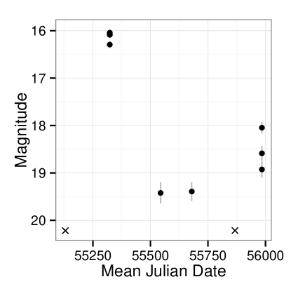
Figure 1: Fragment of a lightcurve. The solid dots represented recorded observations and are plotted with error bars. The two crosses represent times when an observation was attempted but only an upper limit on the magnitude can be specified.

CRTS also includes data from the Mt. Lemon Survey (MLS) which covers mainly a narrow region of the sky near the ecliptic, and Siding Spring Survey (SSS) which covers the Southern hemisphere. We have not included data from MLS or SSS in the current study, but all methods are equally applicable to them as well. About 75% of the sky is covered by CRTS, with parts near the poles and near the plane of our Galaxy excluded. Despite the relative sparsity of the CRTS lightcurves, a strength of the survey is its longevity - we have data where the epochs are spread over 10 years and hence there are parts of the sky with several hundred observations making CRTS one of the richest synoptic datasets. Our technique will scale to much larger datasets including the 500 million lightcurves that CRTS now has. As our method indicates which class an object belongs to based on its lightcurve, we will be able to find matches for known classes. Our measures are sufficiently informative to identify objects that do not belong to known classes by using cluster analysis. This can in turn lead to the discovery of newer classes as well as rarer counterparts of known classes of astronomical objects. CRTS images are available for the entire dataset. When rare or unusual objects are found these can be compared against the images to ensure that no artifacts or spurious features have led to the object being an outlier. The whole process can be automated and human intervention required only at critical junctures like spectroscopic confirmation. Here we apply the method to a large representative sample of transients together with enough non-transients to make the comparisons useful.

Our strategies in deriving these critical measures are 1) selecting a collection of relatively balanced, representative lightcurves of various types and scales (§2); 2) exploring the signatures of these lightcurves (also in §2); 3) developing a Gaussian process regression model for the lightcurves with appropriate priors using astronomical information and an empirical Bayesian approach (§3); and then 4) deriving new measures representing characteristics of the lightcurves using the posterior mean regression curve and residuals. These model-based measures complement existing measures. To examine the power of the new measures in classifying lightcurves in comparison to existing measures, five popular classification procedures are used in four schemes of classification problem in §4: Linear Discriminant Analysis, Decision Trees, Support Vector Machines, Neural Networks, and Random Forests. The results show that our measures perform better than the existing measures. A discussion for why our approach works better is given in §5. Although our modeling approach has been used for an astronomy application, the method could be valuable for other applications involving the classification of sparse, irregularly sampled time series with missing data.

2 Data

We have selected a moderate sample of lightcurves with which to illustrate our methods. The measures available in each lightcurve are Right Acension (RA) and Declination (Dec) which provide the position of the object on the sky, Epoch as Julian Date, magnitude (negative logarithm of flux), an error estimate on the magnitude. The total number of lightcurves considered is 3720. The selection is described below and summarized in Table 1.

We started with just the transients detected by CRTS in real-time over about five years. These include Active Galactic Nuclei (AGNs), Blazars, Cataclysmic Variables (CV), Flare stars and Supernovae (SNe), representing five very different types of lightcurves (e.g. Djorgovski et al. [2011]). We also included a set of 15 random pointings and objects within 3’ of those pointings. These objects are assumed to be non-transients because any transients in there would have been detected earlier. The transients tend to be fainter than typical objects (by definition - it is easier to catch objects that are not normally seen but brighten and become visible for a short duration). In order to offset that, two classes of brighter variable objects were included — Cataclysmic Variables from the Downes set (Downes et al. [2005]) and RR Lyrae which are periodic variables with a period of $\sim$1 day. For the purposes of this article, we have one class called non-transient and seven classes which we call transients viz. AGN, Blazars, CV, Flares, SNe, CV Downes, and RR Lyrae. Note that among the labelled types we have considered here, only the RR Lyrae are periodic. There are methods for distinguishing periodic objects from non-periodic ones but these are not addressed in this article.

Real-world data are much more assymetric and unbalanced than what we have considered here. If we used a simple random sample, there would be very few transients. Training on samples with enough representatives for all classes would be an immense task. We include sufficient non-variables to ensure that the dominant class is represented but not excessively so. In CRTS, the latest catalogs are compared with individual as well as combined catalogs from the archives. The objects that have changed in brightness above a certain threshold (well over a magnitude i.e. approximately a factor of 2.5) are marked as transients. Only a few are found each night compared to millions of nearly non-variable objects.

Functionally transient
Transients					Bright variables
AGN	Blazar	CV	Flare	SNe	CV Downes	RR-Lyrae	non-transient
140	124	461	66	536	376	292	1971

Table 1: Number of lightcurves for each transient type and non-transient objects

The number of observations for each lightcurve varied greatly with a maximum of 641. The median length was 52. We excluded lightcurves with fewer than five observations as these cannot reasonably be classified. The earliest date for any of these lightcurves was 53464 Julian Day (JD) and the latest was 56228, i.e. 5th April 2005 to 28th October 2012. We have used 53464 as our zero-point and referred to all dates as number of days beyond this. Our set spans 2764 days.

An examination of the data is helpful in deciding which methods of analysis may be appropriate. In Figure 2, we see four examples of lightcurves. The objects are identified by their catalogue numbers for reference.

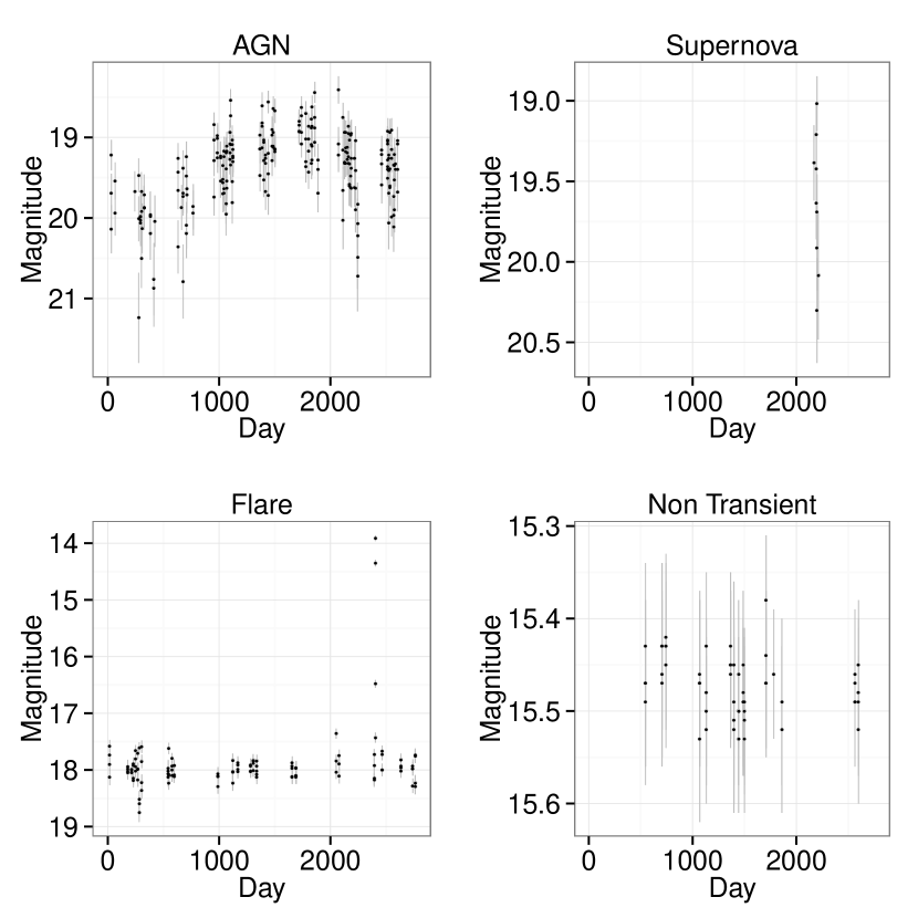
Figure 2: Examples of four lightcurves: (i) CSS071216:110407-045134, an AGN (ii) CSS110405:141104+01115, a Supernova (iii) CSS111103:230309+40060, a Flare and (iv) 301904800767, a non-transient. Note that the range of the vertical axis varies.

Understanding the pattern of measurement is crucial to proper modeling of these curves. The first example shows some gaps in an otherwise dense sequence of measurements. No observations were taken during these periods because the orbit of Earth precluded it. In the second example, there are no observations outside of a narrow range. Observations were attempted at other times but the object was too faint to be observed with a magnitude less than the survey astronomical detection limit of around 20.5. In the third example, we are fortunate that the spike in brightness was observed as this occurs during a brief period of time. In the fourth example, there are quite long periods with no observations but it seems reasonable to assume that no substantial variations in magnitude occurred during these periods given the nearly constant values of magnitude.

It would be useful to know exactly when observations were attempted for given objects while below detection limit. For the purposes of this analysis, we shall assume that all the objects may be surveyed throughout the period of the study but failures to observe have not been recorded. It will be clear how this information could be incorporated into our methods and that this would improve our results in §3.

3 Methods

The nature of the data and the requirements of object classification impose some constraints on what methods are practical. The problem could be viewed as one of functional data analysis (see Ramsay and Silverman [2005]). However, there are several obstacles to pursuing this approach. The observations on the lightcurves are very irregular, both in time and in number. There are methods for dealing with such data but there is a more serious obstacle in that there is little sense in which the curves can be registered or aligned. Excepting the rare case where objects are close in the sky and measurements are likely to be correlated due to atmospheric conditions, lightcurves are independent. This prevents us from using the “borrowing of strength” that registration would allow.

This leads us to another style of analysis based on sample statistics. Judgement is used to devise statistics that measure various characteristics of the observed curves which we may believe important in distinguishing them. We prefer that these measures be relatively simple so that they can be applied quickly and reliably for both short and long lightcurves.

About 20 measures are presented in Richards et al. [2011] that are mostly derived from previous articles. They found these various measures to be helpful in distinguishing objects. Since these measures have been widely tested, at least for brighter data, we use these as a baseline for our analysis. Our objective is to find additional measures that improve the classification accuracy beyond this set. For ease of reference, we will call this set the Richards measures. The specific Richards measures we have used from Table 5 of Richards et al. [2011] are moment-based measures: skew, kurtosis, std and beyond1std, and magnitude-based measures: amplitude, maxslope, mad, medbuf, pairslope and rcorbor, and percentile-based measures: fpr20, fpr35, fpr50, fpr80, peramp and pdfp. We omitted the linear trend measure as this was only large for lightcurves with few observations so it becomes a substitute for a short curve measure. As it happens, including it would not make much difference to the results we present later. We coded these measures from the definitions in Richards et al. [2011].

Although the Richards measures encompass a wide variety of measures, they do not use any concept of modeling the curves. The primary innovation of this paper is to use such modeling to generate additional measures. For lightcurve $i$, we posit a true underlying curve $f_{i}(t)$ that we would see if we could observe the object continuously without error. However, we are able to observe the object only at times $t_{ij}$ for $j=1,\dots n_{i}$. Note that the times of measurement may be almost the same for objects close in the sky but quite different for objects which are farther apart. We observe only $y_{ij}$ for $j=1,\dots n_{i}$. We assume

$$y_{ij}=f_{i}(t_{ij})+\epsilon_{ij}$$ (1)

where the errors $\epsilon_{ij}$ are normal with mean zero but will be correlated.

We considered several methods for estimating $f$ but found that Gaussian process regression was the only satisfactory solution compared to standard non-parametric methods like smoothing splines, kernel smoothing or Lowess for the following reasons:

1. We have censored data - the lightcurve can fall below the detection limit during the range of observation. Standard methods do not deal with this. They can fit curves where we have data but they will not produce sensible fitted curves outside this range.

2. Sometimes we have only a handful of observations and but for other curves we may have hundreds. Simple parametric methods work well with small datasets while larger datasets require the flexibility of nonparametric methods. But Gaussian rocess regression works well for both.

3. We know the measurement error. This information is easily incorporated into the Gaussian process regression but there is no obvious way to take advantage of this information in the standard methods.

3.1 Gaussian Process Regression

See Rasmussen and Williams [2006] for a general introduction. This method requires that we specify a prior for the Gaussian process: $f(x)\sim GP(\psi(x),k(x,x^{\prime}))$. We use the popular squared covariance kernel:

$$k(x,x^{\prime})=\sigma^{2}_{f}\exp\left(-{1\over 2l^{2}}(x-x^{\prime})^{2}\right)+\sigma^{2}_{n}\delta(x-x^{\prime})$$ (2)

where $\delta(x)$ is $0$ when $x\neq 0$ and $1$ when $x=0$. Other reasonable choices of kernel are possible but we found the results were similar (see online appendix for details). One advantage of the Gaussian process approach is that an explicit solution for the posterior is available that can be rapidly calculated. We will need to classify large numbers of future lightcurves as the measurements are collected so we need efficient methods.

There are four components of the prior which must be specified:

1. $\sigma^{2}_{f}$ is the signal variance. A very large fraction of objects to be classified in the future will be non-transients. These non-transients vary in signal but not very much. For this reason, we set $\sigma^{2}_{f}$ to be the median observed variance in the non-transients.

2. $\sigma^{2}_{n}$ is the noise variance. Although it is uncommon in other applications, for astronomical data we are often able to estimate the measurement error. In this example, the measurement error varies a little from case to case. For simplicity, we take the mean observed value of the measurement variance for $\sigma^{2}_{n}$.

3. $l$ is sometimes called the length-scale. It controls the amount of correlation and therefore the amount of smoothness in the resulting posterior fit. We use a value of $140$ days as seen in Figure 3. This choice is based on a subjective assessment on how much smoothness should be expected in these curves. Our classification performance is not very sensitive to this choice.

4. $\psi(x)$ is the prior mean. This choice is challenging and requires further discussion below. We take an empirical Bayes approach.

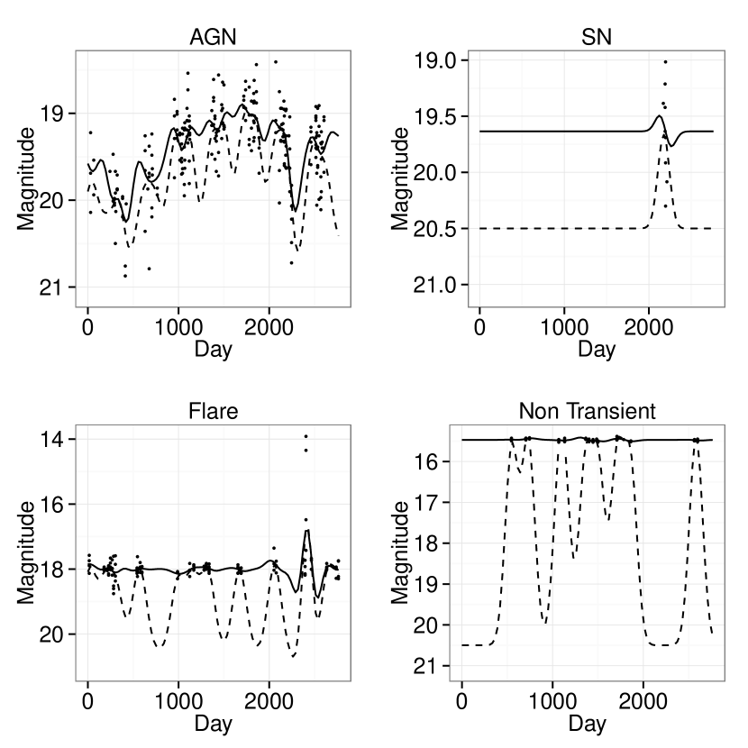
Figure 3: Gaussian process regression fits to lightcurve data. The same four cases as in Figure 2. The solid line fit derives from a prior mean set at the median magnitude while the dashed line fit corresponds to a prior set at a magnitude of 20.5.

We illustrate the issues in setting the prior mean in Figure 3. What values are expected for the curve in regions where there are no measurements? One answer is that we might expect about the same magnitude as that seen elsewhere for this object. This suggest setting the prior to the median magnitude for the object. This choice can be seen in the solid line fits in Figure 3. This works well enough in three cases but fails for the supernova example because we do not expect this curve to follow a similar magnitude at other times. If it did, it would have been seen. So an alternative approach is to set the prior to the detection limit at a magnitude of 20.5. This gives the dashed line fits as seen in Figure 3. This works well for the supernova case but is problematic for the other three curves. In regions of no measurement, the fitted curve is drawn down towards the detection limit. We can counteract this by increasing the length-scale (i.e. increasing the smoothness in the prior) but tends to attenuate real effects and still does not work well for relatively sparsely measured curves (such as the non-variable in this example).

Our solution is to use an adaptive prior. When there is less than one year of observations, we use the detection limit, otherwise we use the median magnitude. The choice of a year is large enough that sparse but widely measured curves such as the fourth example do not use the detection limit. But the choice is small enough that the detection limit is used in cases like the third example. Now using the data to select the prior may make our method at least partly empirical Bayes rather than pure Bayes, but we need to judge the method by its classification performance which is improved by this choice.

3.2 Curve Measures

Given the posterior mean $\hat{f}$, we compute fitted curve measures from $\hat{f}_{i}$ for curve $i$ computed on an evenly spaced grid of values on the range of observation $u_{j}$ for $j=1,\dots,m=300$. The italicized word is the name of the variable for future reference:

• totvar total variation: $\sum_{j}|\hat{f}_{i}(u_{i,j+1})-\hat{f}_{i}(u_{ij})|/m$

• quadvar quadratic variation: $\sum_{j}(\hat{f}_{i}(u_{i,j+1})-\hat{f}_{i}(u_{ij}))^{2}/m$

• famp amplitude of fitted function: $\max_{t}\hat{f}_{i}-\min_{t}\hat{f}_{i}$.

• fslope maximum derivative in the fitted curve: $\max_{t}|\hat{f}^{\prime}_{i}|$

We also use the maximum in absolute value of the scaled residuals from the fit, called outl, as a measure.

Another feature of this data is the clustering of times of measurement which can occur in groups of up to 4 observations that are spaced by ten minutes within a thirty minute period. The Gaussian process regression is not able to model the variation at this finer scale because setting the length-scale $l$ to a much smaller value would result in too rough a fit overall. We need another set of measures to capture the characteristics at this scale of measurement.

We compute the mean within each of these groups of up to four observations as $\breve{f}_{ij}$ and then compute the following measures:

• lsd: the log of the standard error, $\breve{\sigma}$, computed using the residuals from these group mean fits.

• gtvar: The group total variation $\sum_{j}|\breve{f}(t_{i,j+1})-\breve{f}(t_{ij})|/n_{i}$

• gscore $\sum_{j}\phi((\breve{f}_{ij}-\bar{f}_{i})/\breve{\sigma})/n_{i}$ where $\phi$ is the standard normal density, $\bar{f}$ is mean of the fitted group means.

The last measure is motivated by scoring methods used to judge prediction performance.

There are also some gaps within the Richards measures set of sample curve summary measures. We add the following:

• shov mean of absolute differences of successive observed values:
  $\sum_{j}|y_{i,j+1}-y_{ij}|/n_{i}$

• maxdiff the maximum difference of successive observed values:
  $\max_{j}|y_{i,j+1}-y_{ij}|$

• dscore the density score: $\sum_{j}\phi((y_{ij}-\tilde{f}_{i})/s_{ij}))/n_{i}$ where $\tilde{f}_{i}$ is the median observed magnitude for curve $i$ and $s_{ij}$ is the observed measurement error at $t_{ij}$.

There are other measures that may be informative for the current data we are analyzing but may not have predictive value in future examples. We have avoided using such measures. They fall into three categories:

1. Measures based on the number of observations in a lightcurve. Some phenomena, such as supernovae, are not recurrent and subsequent observations may fall below the observable limit. Lightcurves in such cases can be quite short but this is known only in retrospect so this is not usefully predictive. The number of observations does have some impact on the choice of prior and in scaling some of the measures, but we refrain from using this number (or anything closely related) as a direct measure for classification purposes.

2. The classification of an object should be invariant to the addition of a constant to the observed magnitudes. But some biases in the way that our example data was extracted would cause, say, the mean magnitude, to be an effective discriminator among the types. This mean magnitude will not be reproducible in future samples so we do not use this measure or anything related to it.

3. Location in the sky. The method of constructing our example dataset would mean that location would become useful discriminator. As it happens, location would provide some usable information for classification as extra-galactic objects are more likely to appear away from the galactic plane but we refrain from using this information here.

There is additional information such as the nearest radio source or the nearest galaxy which could also be useful in classification but we do not use here. We experimented with a larger set of additional measures (as can be seen in the online appendix) but we have presented only those that appear to have some additional value for classification.

Given this set of measures, we can use any number of classification methods to distinguish objects using lightcurves. We demonstrate the use of our measures using five popular classification methods. We will generally use the default choice of options for the particular implementation in $R$. Our objective is to show that our measures represent an improvement over using the Richards measures alone. It is likely that the classification methods could be better tuned to obtain a better result or that the reader may favor another classification method. But that is not the point of this article. We are not trying to claim one classification method is better than another, just that our measures are better.

The methods we have used are:

LDA

Standard linear discriminant analysis method as implemented in Venables and Ripley [2002].

TREE

Recursive partitioning as implemented in the rpart package by Therneau et al. [2013].

SVM

Support vector machines as implemented in the kernlab package by Karatzoglou et al. [2004].

NN

Neural network as implemented in the nnet package by Venables and Ripley [2002]

RF

Random forest ensemble implemented by the randomForest package by Liaw and Wiener [2002]

We log-transformed the measures that have extreme skewness in order to improve classification performance. The same transformations were used in all the comparisons below. Without these transformations, both sets of measures would perform less well in general for methods LDA, SVM and NN. The partitioning-based methods, TREE and RF, are invariant to monotone transformations. Explicit details of the implementation can be found in the Appendix.

4 Results

Classification methods usually do not perform as well as expected when applied to new data. When the same data are used to both fit and evaluate a method, the classification rate is inflated. To avoid this problem, we randomly split the data into 2/3 for training i.e. used to develop the classification rule and 1/3 for testing, that is to evaluate how well the rule performs. Since we are only interested in the relative performance of the classification measures and methods and because the sample size is relatively large, we present only one random split. In the online appendix, we repeat the calculations for 100 random splits and the results are not qualitatively different.

4.1 Classification Performance

We considered four different types of classification problem with bold labels used for future reference:

All

The overall problem of classifying eight types — the non-transients and the seven transient types.

Transient or not

Perhaps the first step in any lightcurve classification process will be to determine which objects are transient.

Transient only

Having separated out the non-transients, the next step might be to identify the type of the transient. For this problem, we delete the non-transients from both the test and training data.

Heirarchical

An alternative approach to classifying all objects directly is to first classify objects into transient or not transient, then if transient to classify among the seven available types.

We show the percentages correctly classified using the Richards measures in Table 2 and using our measures (which incorporate the Richards set) in Table 3.

	LDA	TREE	SVM	NN	RF
All	56.7	58.6	66.1	63.3	67.3
Transient or not	74.7	79.5	81.0	75.2	82.5
Transient only	54.5	58.9	64.4	60.1	62.9
Heirarchical	56.4	60.4	64.7	58.8	65.6

Table 2: Percentage correctly classified using the Richards measures.

	LDA	TREE	SVM	NN	RF
All	76.0	71.9	80.2	79.6	80.5
Transient or not	90.4	88.4	92.0	91.6	91.8
Transient only	70.1	65.1	74.3	72.3	74.2
Heirarchical	76.0	72.7	79.9	78.5	79.8

Table 3: Percentage correctly classified using our measures in addition to the Richards set.

The standard error for the classification rate is just less than 1% which is helpful in judging which differences are notable in these tables. Table 2 and Table 3 show that our measures provide a significant improvement to the Richards measures alone which might be regarded as the previous state of the art. Of course, adding additional measures can only improve the fit of a model, but we are using an independent test set so we can be sure the improvement is more than illusory. There is little to distinguish the heirarchical approach from the one-step method although we would recommend the heirarchical approach on an unbiased sample of lightcurves because these would be dominated by non-variables.

Tables 4 and 5 show the numbers of objects classified into all eight types compared to their actual types. We present only the random forest results as this was the best performing method. The most noticeable differences between the two sets of measures is that our method results in classifications in all eight types while the older set fails to classify any objects into four of the types. Since the Downes set is just another form of CV, we not so concerned about a failure to distinguish these two. We can see that Flares are hard to identify.

	Actual types
Predicted	AGN	Blazar	CV	Downes	Flare	NT	RR-Lyrae	SNe
AGN	0	0	0	0	0	0	0	0
Blazar	0	0	0	0	0	0	0	0
CV	5	26	95	53	4	20	3	27
CV Downes	0	0	0	0	0	0	0	0
Flare	0	0	0	0	0	0	0	0
non-transient (NT)	31	7	26	73	16	497	47	80
RR-Lyrae	0	1	2	3	0	12	53	3
SNe	8	5	22	6	4	29	0	82

Table 4: Confusion matrix for the Richards set using random forest classification of all eight types. The rows are the predicted types while the columns are the actual types.

	Actual types
Predicted	AGN	Blazar	CV	Downes	Flare	NT	RR-Lyrae	SNe
AGN	31	3	0	2	0	2	0	2
Blazar	0	27	3	7	0	0	0	0
CV	2	4	93	26	0	4	2	14
CV Downes	1	2	15	58	0	7	5	0
Flare	0	0	0	3	8	0	0	0
non-transient (NT)	8	0	9	25	15	541	1	16
RR-Lyrae	0	1	0	7	0	0	95	0
SNe	2	2	25	7	1	4	0	160

Table 5: Confusion matrix for our measures using random forest classification of all eight types. The rows are the predicted types while the columns are the actual types.

Our sample heavily over-represents transients which would constitute less than 1% of an unbiased sample. Hence, even a null method which classified randomly based on prior proportions would achieve around 99% accuracy. Certainly any sensible method will do even better than this and it would take a very large unbiased sample to distinguish different methods. This explains why we have used a more balanced, although biased, representation of the eight types. Similar strategies are used in case-control studies.

Because these classification methods will be applied to very large numbers of objects, even quite low error rates will result in large numbers of misclassified objects resulting in wasted resources or missed opportunities. For this reason, the primary classification into transient against non-transient is particularly important. We can see our proposed measures perform well in this respect, halving the previous error rate, although there remains further room for improvement.

4.2 Testing on Fresh Data

We verified the performance of our measures by applying the methodology to two datasets distinct from the training set. We assembled 574 transients that have been more recently manually classified consisting of the types AGN, Blazar, CV, Flare and SNe. This is a complete set of CSS transients from 2013 where astronomers using additional auxiliary data were reasonably confident of the nature of the transient. We used all the objects of these five types from the original set of data (updating them to include more recently collected observations to match the lightcurve durations) to train classification rules. We then applied these rules to a test set formed from the recent set of transients. The classification rates from this exercise a shown in Table 6. The addition of our set of measures results in an improved performance over the Richards set alone.

	LDA	TREE	SVM	NN	RF
Richards	60.8	64.0	72.6	71.1	73.1
Ours+Richards	74.6	67.4	78.0	77.2	79.0

Table 6: Percentage of the new set of five transient types correctly classified.

We also assembled a large set of 100,000 lightcurves from CSS. We sampled 50,000 objects from $0<S_{J}<0.01$ and labeled these non-variables, and 50,000 more from $0.5<S_{J}<1$ which we labeled as variable. Any labeling based on a single variable will not be entirely reliable so we have chosen ranges from the extremes of $S_{J}$ to increase confidence that the labels are correct. See Drake et al. [2014] for background. Very few of the variables are likely to be transients and most of them will be of types not already considered earlier. We randomly divided the data into two equal parts. One half was used to train classification rules and the other half to test the performance. The classification rates are shown in Table 7 where we see that the addition of our set of measures to the Richards set greatly improves the rates.

	LDA	TREE	SVM	NN	RF
Richards	75.5	79.4	85.3	76.8	85.5
Ours+Richards	97.5	89.2	98.4	98.3	96.8

Table 7: Percentage of 50,000 variables and non-variables correctly classified.

4.3 Feature Selection

The random forest method provides a means of determining the worth of predictors. Suppose that within a particular node, the proportion classified as type $i$ is given by $p_{i}$. The Gini index is defined as $1-\sum_{i}p_{i}^{2}$ and can be used as a measure of node impurity. We can see how much the Gini index averaged across nodes decreases when a measure is removed from the current set. We remove the measure which leads to the least decrease. We refit the model with the reduced set and repeat the process until all measures have gone. The classification rate after each measure is removed is shown in Figure 4 for the problem of classifying all 8 types. See also Donalek et al. [2013] for similar procedures.

There is little difference in classification accuracy between the training and test datasets which is a good indication that we are not over-fitting. We see that this selection process removes most of the older non-model based measures without any noticeable loss in classification accuracy. Our fitted curve measures quadvar, famp, totvar and fslope are among the most useful classification variables. Hence we can see that deriving measures based on our model is a good place to start and not merely a way to supplement existing older measures. The message from the other three classification problems is similar. We do not propose that the older measures be discarded as they are generally simple to compute and may be useful in new situations.

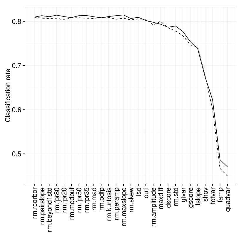
Figure 4: Stepwise selection of measures. The classification rates (solid for the training set and dashed for test set) are shown after the named measure is removed from the model. The order in which the measures are removed is determined by the least decrease in the Gini index. Measures from the Richards set have the prefix rm.

5 Discussion

We have presented two advances. In Statistics, we have shown how Gaussian process regression can be adapted and the corresponding priors developed to deal with data of varying sampling density, structures and scales. We are able to deconvolute the underlying curves $f_{i}$ and measurement noise $\epsilon_{i}$ to distinguish the objects rather than use summary statistics that use samples $y_{ij}$ with mixed up noise and signal. With some further effort we might show that the measures based on our estimated curves, under some regularity conditions, would be consistent for the features of the true underlying curves. A summary statistic-based approach can be biased or inconsistent for these measures. In Astronomy, we have demonstrated a new method of generating measures representing features of lightcurves that are significantly better in classifying objects than previous methods.

There is further scope for improvement in performance by optimising the classification using routine methods. With more detailed information about when locations were surveyed but no object observed, we can further refine our priors to obtain superior results. The measures we have developed are now being used for several purposes. We can apply the method for new data where the location has only been surveyed for a shorter period of time. The measures can all be scaled appropriately. We have experimented by taking time-wise subsets of this data and have found that although the absolute performance drops with shorter curves, the relative performance over the older set of measures remains. Furthermore, the measures provide the means to detect objects of unknown type. By adding a richer and more powerful set of measures, we have increased the potential for such interesting discoveries. Some of our measures have already been used in classifying new lightcurves.

Appendix

Our data, code and detailed results are available as a supplement to be found at
people.bath.ac.uk/jjf23/modlc

References

- Blocker and Protopapas [2013] A. W. Blocker and P. Protopapas. Semi-parametric robust event detection for massive time-domain databases. arxiv:1301.3027, 2013.
- Blomme et al. [2010] J. Blomme et al. Automated Classification of Variable Stars in the Asteroseismology Program of the Kepler Space Mission. The Astrophysical Journal Letters, 713(2):L204–L207, 2010.
- Bloom et al. [2012] J. S. Bloom et al. Automating discovery and classification of transients and variable stars in the synoptic survey era. PASP, 124, 1175, 2012.
- Borne [2009] K. Borne. Scientific data mining in astronomy. arXiv:0911.0505, 2009.
- Ciardi et al. [2011] D. R. Ciardi et al. Characterizing the Variability of Stars with Early-release Kepler Data. The Astronomical Journal, 141(4):108, 2011.
- Djorgovski et al. [2011] S. Djorgovski et al. The Catalina Real-Time Transient Survey (CRTS). arXiv:1102.5004, 2011.
- Djorgovski et al. [2012] S. G. Djorgovski et al. Flashes in a star stream: Automated classification of astronomical transient events. 2012 IEEE 8th International Conference on E-Science, 2012. doi: http://doi.ieeecomputersociety.org/10.1109/eScience.2012.6404437.
- Donalek et al. [2013] C. Donalek et al. Feature selection strategies for classifying high dimensional astronomical data sets. CoRR, abs/1310.1976, 2013.
- Downes et al. [2005] R. Downes et al. A catalog and atlas of cataclysmic variables: The final edition. Journal of Astronomical Data, 11:2, 2005.
- Drake et al. [2009] A. Drake et al. First Results from the Catalina Real-time Transient Survey. The Astrophysical Journal, 696:870–884, 2009.
- Drake et al. [2014] A. J. Drake et al. The Catalina Surveys Periodic Variable Star Catalog. arXiv:1405.4290, 2014.
- Graham et al. [2014] M. J. Graham et al. A novel variability-based method for quasar selection: evidence for a rest-frame ∼54 d characteristic time-scale. MNRAS, 439, 703, 2014.
- Karatzoglou et al. [2004] A. Karatzoglou et al. kernlab – an S4 package for kernel methods in R. Journal of Statistical Software, 11(9):1–20, 2004. URL {http://www.jstatsoft.org/v11/i09/}.
- Liaw and Wiener [2002] A. Liaw and M. Wiener. Classification and Regression by randomForest. R News, 2(3):18–22, 2002. URL {http://CRAN.R-project.org/doc/Rnews/}.
- Mahabal et al. [2011] A. Mahabal et al. Discovery, classification, and scientific exploration of transient events from the Catalina Real-time Transient Survey. BASI, 2011, 39, 387-408, 2011.
- Peng et al. [2012] N. Peng et al. Selecting quasar candidates using a support vector machine classification system. Monthly Notices of the Royal Astronomical Society, 425(4):2599–2609, 2012.
- Ramsay and Silverman [2005] J. Ramsay and B. Silverman. Functional Data Analysis. Springer, New York, 2 edition, 2005.
- Rasmussen and Williams [2006] C. Rasmussen and C. Williams. Gaussian Processes for Machine Learning. MIT Press, Cambridge, 2006.
- Richards et al. [2011] J. Richards et al. On Machine-Learned Classification of Variable Stars with Sparse and Noisy Time-Series Data. The Astrophysical Journal, 733(1):23, 2011.
- Richards et al. [2012] J. W. Richards et al. Active learning to overcome sample selection bias: Application to photometric variable star classification. ApJ, 744, 192, 2012.
- Therneau et al. [2013] T. Therneau, B. Atkinson, and B. Ripley. rpart: Recursive Partitioning, 2013. R package version 4.1-1.
- Venables and Ripley [2002] W. N. Venables and B. D. Ripley. Modern Applied Statistics with S. Springer, New York, fourth edition, 2002. URL {http://www.stats.ox.ac.uk/pub/MASS4}.