Dynamical modeling of tidal streams

Abstract

I present a new framework for modeling the dynamics of tidal streams. The framework consists of simple models for the initial action–angle distribution of tidal debris, which can be straightforwardly evolved forward in time. Taking advantage of the essentially one-dimensional nature of tidal streams, the transformation to position–velocity coordinates can be linearized and interpolated near a small number of points along the stream, thus allowing for efficient computations of a stream’s properties in observable quantities. I illustrate how to calculate the stream’s average location (its “track”) in different coordinate systems, how to quickly estimate the dispersion around its track, and how to draw mock stream data. As a generative model, this framework allows one to compute the full probability distribution function and marginalize over or condition it on certain phase–space dimensions as well as convolve it with observational uncertainties. This will be instrumental in proper data analysis of stream data. In addition to providing a computationally-efficient practical tool for modeling the dynamics of tidal streams, the action–angle nature of the framework helps elucidate how the observed width of the stream relates to the velocity dispersion or mass of the progenitor, and how the progenitors of “orphan” streams could be located.

The practical usefulness of the proposed framework crucially depends on the ability to calculate action–angle variables for any orbit in any gravitational potential. A novel method for calculating actions, frequencies, and angles in any static potential using a single orbit integration is described in an Appendix.

1. Introduction

Tidal streams hold enormous promise as probes of both the large-scale structure of the Milky Way (MW) halo’s density distribution (e.g., Johnston et al., 1999; Koposov et al., 2010) and its small-scale fluctuations (Carlberg, 2012). However, two factors have hampered the practical use of tidal streams in obtaining constraints on the MW gravitational potential. First, streams do not trace a single orbit, which has led to confusion over how to best fit streams and over how problematic the single-orbit approximation really is (Eyre & Binney, 2011; Sanders & Binney, 2013a). Second, approaches that go beyond the single-orbit assumption encounter practical difficulties of computational cost and observational data quality making many of these approaches impractical for real, noisy data (Law et al., 2005; Sanders & Binney, 2013b; Price-Whelan & Johnston, 2013). Observed gaps in tidal streams may be due to interactions with dark–matter subhalos (Yoon et al., 2011), but underdensities could also be created by the dynamics of stream stars (Küpper et al., 2010). This hinders our ability to use underdensities in star counts along a tidal stream in order to constrain the number of encounters with dark satellites and their masses (Ngan & Carlberg, 2014). Simple, analytic models of how tidal streams are generated—generative models—would greatly benefit both of these applications.

It has long been clear that the dynamics of tidal streams is most simply described in terms of action–angle coordinates (Tremaine, 1999; Helmi & White, 1999). Once a star has been tidally stripped from the progenitor, the self-gravity of the stream can be neglected and the orbital actions of a stream member are conserved while the angles increase linearly with time. The action–angle structure of a stream is therefore characterized by strong but straightforward correlations between the actions and angles of stream members, the exploitation of which is crucial for using streams to measure the host gravitational potential (Sanders & Binney, 2013b). The description of a stream in action–angle coordinates also elucidates the connection between the orbit and velocity dispersion (or mass) of the progenitor and the action distribution of the tidal debris (Eyre & Binney, 2011), allowing simple physical models of the stream to be used and to be constrained by observational data.

However, streams are observed in position–velocity coordinates and for action–angle descriptions to be useful, we must be able to calculate the transformation between these coordinate systems efficiently. Until now this has required accurate phase–space data and specialized algorithms that break down for the eccentric orbits on which tidal-stream progenitors are typically found (that is, radial and/or vertical actions of similar magnitude as the angular momentum; Sanders 2012). However, even with Gaia (Perryman et al., 2001), all of the phase–space coordinates except for the sky position will typically have non-negligible uncertainties compared to the intrinsic dispersion of the stream and in particular the line-of-sight velocities of the faintest stream members will not be observed for many stars. Additionally, streams are superimposed on a non-negligible background of field stars and background contamination cannot be easily taken into account in any of the current stream-fitting methods.

In this paper, I present a new method for modeling tidal streams that fundamentally lives in frequency–angle space, because the stream distribution function is essentially one-dimensional in this space. While many of the results of this paper are more generally valid, the fiducial stream model in this paper consists of a three-dimensional (close to) Gaussian distribution of frequencies in the stream, a three-dimensional Gaussian distribution of initial angle offsets between stream members and the progenitor, and a uniform distribution of stripping times; the frequency and angle offset distributions are independent of stripping time. While this model oversimplifies the real stripping process, I hypothesize that at least for constraining the gravitational potential with stream data, this simple model is likely unbiased. For detailed mock stream data, more elaborate models of the stripping process as a function of time might be necessary and I discuss how these could easily be incorporated into the proposed framework.

To evaluate the model in position–velocity coordinates, the transformation to and from action–angle coordinates is computed using a novel method for calculating action–angle coordinates presented in Appendix A. This transformation is linearized at a small number of points near the stream that span its length. For streams originating from progenitors with masses $\lesssim 10^{8}\,\mathrm{M}_{\odot}$, the separation between the stream track and the progenitor orbit as well as the internal differences within the stream are small, such that the linear approximations used here are accurate enough. The linear approximation allows for fast evaluation of the average stream location (the stream “track”) in position–velocity coordinates and efficient mock data generation. For a uniform distribution of stripping times, an observed stream member’s phase–space probability distribution function (PDF) can be analytically marginalized over stripping time, such that using the linear approximation any evaluation—including marginalization and uncertainty convolution—of the PDF is extremely rapid. This clears the way for proper probabilistic inference of the Milky Way halo’s gravitational potential and progenitor properties using stream data for individual stars.

The framework presented in this paper differs from other approaches that model streams in action–angle coordinates in a few respects. As in Helmi & White (1999), the model is a generative one in that it gives an analytic prescription for the initial action–angle distribution of tidal debris that is then evolved in time to generate a tidal stream. The difference between these two generative models is that I propose simple, few-parameter models for the initial action–angle distributions, that I work out the properties of streams in observable coordinates in more detail, and that I present and use a general action–angle transformation that allows stream modeling in general potentials. The average location of a stream in phase-space can be computed in the framework presented here and it could be used to replace orbit fitting; Varghese et al. (2011) discussed a similar method to model observed streams. The method in this paper differs from that of Varghese et al. (2011) in that the model is fundamentally located in action–angle space rather than position–velocity space and in that the width and length of the stream are related to the offsets between the stream, the progenitor’s orbit, and the average orbit as a function of stream position. Thus, the present framework does not have to assume a progenitor velocity dispersion, but can constrain it from the stream data as well. My approach differs from the framework of Johnston (1998), which is also a generative model, in that it lives in action–angle space rather than energy–angular-momentum space and that it can be applied to arbitrary time-independent potentials rather than just spherical potentials close to a logarithmic potential.

This paper is outlined as follows. In $\mathsection$ 2 I briefly summarize the dynamics of tidal streams in terms of action–angle coordinates. A generative model of a tidal stream in frequency–angle coordinates is given in $\mathsection$ 3. $\mathsection$ 4 describes how to compute the stream’s properties as a function of angle along the stream, both in action–angle coordinates and in position–velocity coordinates. $\mathsection$ 5 discusses how to generate mock stream data using the generative model of a tidal stream and in $\mathsection$ 6 I show how to calculate the stream PDF for individual stream members as well as its marginalization and convolution over missing and noisy directions. A discussion and outlook is presented in $\mathsection$ 7 and I conclude in $\mathsection$ 8. In Appendix A I review the method of Fox (2012) for calculating actions in any static gravitational potential and I show how it can be simplified and extended to compute frequencies and angles.

2. The dynamics of tidal streams

The dynamics of tidal streams both in position–velocity and action–angle space has been described previously by various authors (e.g., Helmi & White, 1999; Tremaine, 1999; Johnston, 1998; Sanders & Binney, 2013a). I provide here a brief description of the dynamics of tidal streams that is relevant for what follows.

In position–velocity space, a tidal stream forms as stars are stripped from a progenitor cluster or satellite galaxy some time $t_{s}>0$ in the past and then evolve (largely) independently in a galaxy’s host potential, moving away both in position and velocity from the progenitor object as time goes on. Thus, a star was offset by a small amount $(\Delta\mathbf{x},\Delta\mathbf{v})$ from the position of the progenitor $(\mathbf{x}^{p},\mathbf{v}^{p})(-t_{s})$ at that time. Then the star orbited under the influence of the same gravitational potential $\Phi$ as the progenitor until the present day $(t=0)$, when it was observed: $(\mathbf{x},\mathbf{v})(t=0)$ = $\mathbf{H}_{t_{s}}(\mathbf{x}^{p}(-t_{s})+\Delta\mathbf{x},\mathbf{v}^{p}(-t_{s})+\Delta\mathbf{v})$, where $\mathbf{H}$ denotes the Hamiltonian flow from $t=-t_{s}$ to $t=0$ (see Binney & Tremaine 2008); this is simply the orbit of the star between these times. In phase-space this orbit can be calculated by solving Hamilton’s equations: $\dot{\mathbf{x}}=\mathbf{v};\dot{\mathbf{v}}=-\mathrm{d}\Phi/\mathrm{d}\mathbf{x}$.

In action–angle space the dynamics of stream formation is much simpler. A star received an offset ($\Delta\mathbf{J},\Delta\boldsymbol{\theta}$) at time $-t_{s}$ from the action–angle coordinates of the progenitor $(\mathbf{J}^{p},\boldsymbol{\theta}^{p})$, similar to the small offset ($\Delta\mathbf{x},\Delta\mathbf{v})$. The offset in the actions corresponds to an offset in the frequencies $\Delta\mathbf{\Omega}$; ultimately, this frequency offset is responsible for the spreading of the stream over long stretches on the sky. Because both the progenitor’s angles and the star’s angles increase linearly with time, albeit at different frequencies, the difference in the angles also increases linearly in time. Therefore at time $t=0$ the difference in angles is

$$\Delta\boldsymbol{\theta}(t=0)=\Delta\boldsymbol{\theta}(-t_{s})+\Delta\mathbf{\Omega}\,t_{s}\,,$$ (1)

while the difference in actions is constant

$$\Delta\mathbf{J}(t=0)=\Delta\mathbf{J}(-t_{s})\,.$$ (2)

As the initial offset $\Delta\boldsymbol{\theta}(-t_{s})$ in angles is small compared to the growth $\Delta\mathbf{\Omega}\,t_{s}$, we have that $\Delta\boldsymbol{\theta}(t=0)\approx\Delta\mathbf{\Omega}\,t_{s}$.

Thus, in action–angle coordinates, the dynamics of tidal-stream formation is simplified to linear growth of small initial angle differences due to small action/frequency differences. The angle direction $\mathbf{\hat{\mathbf{\Omega}}}\equiv\Delta\mathbf{\Omega}/|\Delta\mathbf{\Omega}|$ along which a star moves away from the progenitor is related to the initial action offset by $\Delta\mathbf{\Omega}\approx(\partial\mathbf{\Omega}/\partial\mathbf{J})\Delta\mathbf{J}=(\partial^{2}H/\partial\mathbf{J}\partial\mathbf{J})\Delta\mathbf{J}$, in the limit of small action offsets, because $\mathbf{\Omega}=\partial H/\partial\mathbf{J}$, where $H$ is the Hamiltonian. For an approximately one-dimensional stream to form, the Hessian matrix $(\partial^{2}H/\partial\mathbf{J}\partial\mathbf{J})\large|_{\mathbf{J}^{p}}$ has to be dominated by a single large eigenvalue; in this case the angle difference of stars stripped from the stream at any time will fall along approximately the same direction $\mathbf{\hat{\mathbf{\Omega}}}$, and the stream will be essentially one dimensional. In detail, because the distribution of initial offsets $\Delta\mathbf{J}$ is not isotropic, the direction $\mathbf{\hat{\mathbf{\Omega}}}$ is not just determined by the potential (through $H$) and the progenitor orbit $\mathbf{J}^{p}$, but also by the distribution of $\Delta\mathbf{J}$, which is set through a combination of the internal dynamics of the progenitor and the stripping process.

3. Generative models of tidal streams

3.1. A simulation

I illustrate the theoretical considerations set forth in this paper by using a simulated tidal stream. This stream is set up similarly to that used in Sanders & Binney (2013b). The stream is constructed by running an $N$-body simulation of a King cluster (King, 1966) on an orbit similar to that of the GD-1 stream (Koposov et al., 2010). Specifically, a King cluster with a mass of $2\times 10^{4}\,\mathrm{M}_{\odot}$, a tidal radius of $0.07\,\mathrm{kpc}$, and a ratio of the central potential to the velocity dispersion squared of $2.0$ is sampled using $10^{4}$ particles. The cluster is evolved with self-gravity in an external logarithmic host potential with $V_{c}=220\,\mathrm{km\ s}^{-1}$ and a flattening $q=0.9$ ($\Phi=V_{c}^{2}\ln[R^{2}+z^{2}/q^{2}]$) using the gyrfalcon code (Dehnen, 2000, 2002) with a softening of $1.5\,\mathrm{pc}$ in the NEMO toolkit (Teuben, 1995). The cluster is evolved for $5.011\,\mathrm{Gyr}$ ($=5.125\,\mathrm{kpc}/[\,\mathrm{km\ s}^{-1}]$) from the initial condition $(X,Y,Z)=$ $(-11.63337239$ $,-20.76235661,$ $-10.631736273934635)\,\mathrm{kpc}$ and $(V_{X},V_{Y},V_{Z})=$ $(-128.8281653$ $,42.88727925,$ $79.172383882274971)\,\mathrm{km\ s}^{-1}$, chosen such that the cluster ends up at roughly the observed location of the GD-1 stream at the end of the simulation (Koposov et al., 2010). The progenitor cluster’s orbit has an eccentricity of $0.31$, a pericenter of $13.7\,\mathrm{kpc}$, and a current $r=14.4\,\mathrm{kpc}$, such that the cluster is close to pericenter at the end of the simulation. The actions of the progenitor are $(J_{R},L_{Z},J_{Z})=(288.5,-3173.7,897.6)\,\mathrm{kpc}\,\mathrm{km\ s}^{-1}$ and its orbital frequencies are $(\Omega_{R},\Omega_{\phi},\Omega_{Z})=(15.7,-10.8,11.9)\,\mathrm{Gyr}^{-1}$.

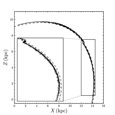
Figure 1.— Mock tidal stream simulated as described in $\mathsection$ 3.1 after $5.011\,\mathrm{Gyr}$ of evolution in Galactocentric $X$ and $Z$ coordinates. The gray dot shows the current position of the progenitor cluster and the dashed line shows its orbit. The solid line gives the stream track, calculated using the method described in $\mathsection$ 4. The inset shows a zoomed-in version of part of the leading stream (stretched in $X$ and $Z$) that more clearly shows the offset between the stream track and the progenitor orbit.

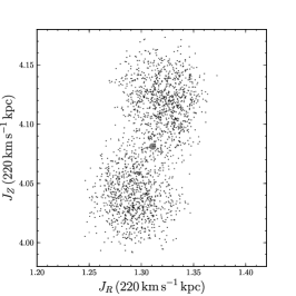
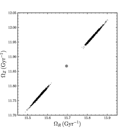
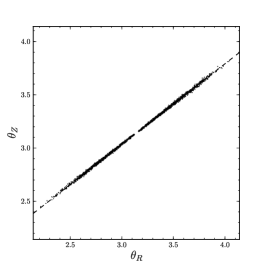
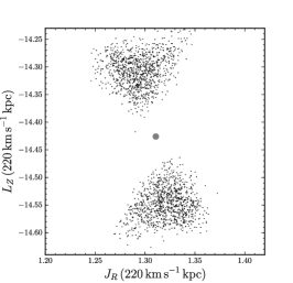
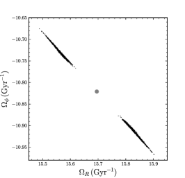
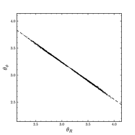
Figure 2.— Simulated tidal stream from $\mathsection$ 3.1 after $5.011\,\mathrm{Gyr}$ of evolution in action–frequency–angle coordinates. The top row displays projections of the actions (left), frequencies (middle), and angles (right) in the $R$ and $Z$ directions; the bottom panels shows the same for $R$ and $\phi$. While the action distribution has a quite complicated form, the frequency distribution is close to one-dimensional and the leading and trailing parts of the stream clearly separate (the two clouds in action–action and frequency–frequency correspond to the leading and trailing arm). In the right panels, the angles of the progenitor have each been shifted to $\pi$ and the dashed lines show the direction of the progenitor’s frequency vector. The misalignment between the progenitor’s frequency vector and the mean frequency-offset vector of the debris is $0.18^{\circ}$.

The final position of the stream in $(X,Z)$ is shown in Figure 1. Figure 2 shows the final position of the stream in action–frequency–angle coordinates, calculated using the algorithm described in Appendix A. As described in $\mathsection$ 2, a one-dimensional tidal stream forms because even though the action distribution of the tidal debris is not isotropic or one-dimensional, the Hessian $(\partial^{2}H/\partial\mathbf{J}\partial\mathbf{J})\large|_{\mathbf{J}^{p}}$ is so strongly dominated by a single large eigenvalue (the ratio of the largest to the second largest eigenvalue is about $30$), that the frequency distribution of the debris is essentially one dimensional. The angle distribution of the debris at the end of the simulation is therefore essentially one dimensional as well.

3.2. A model in frequency–action space

The action and frequency distributions shown in Figure 2 combined with the knowledge that for any tidal stream the Hessian $(\partial^{2}H/\partial\mathbf{J}\partial\mathbf{J})\large|_{\mathbf{J}^{p}}$ must be strongly dominated by a single large eigenvalue leads me to propose that frequency–angle space is a better coordinate system than action–angle space for modeling tidal streams. That is, the distribution of actions in a tidal stream has a complicated structure that is hard to capture using a simple, analytic form (see also the discussion in Eyre & Binney 2011). Especially the “bow tie” structure in $(J_{R},L_{Z})$ and the overlapping leading- and trailing-arm distributions in ($J_{R},J_{Z}$) are difficult to model with a simple distribution function. The distribution of frequencies, however, is close-to one dimensional, its direction of largest variance can be well-modeled as a Gaussian (although below we will model it slightly differently), and its parameters can all be easily estimated from the velocity dispersion of the progenitor, the orbit of the progenitor, and the gravitational potential, as discussed below. Therefore, we will model tidal streams in frequency–angle space. Because the leading and trailing arm are well-separated in frequency space, we model each arm individually.

A generative model of a tidal stream in frequency–angle space requires three ingredients: (a) a model for the distribution of times at which stars are stripped from the progenitor, (b) a prescription for the distribution of frequency offsets from the progenitor at every given stripping time, and (c) a description of the angle offsets for any given frequency offset and stripping time. Having specified these ingredients, we can then generate tidal debris at any given stripping time and evolve it forward using the simple linear dynamics in frequency–angle space discussed in $\mathsection$ 2. The initial angle offsets are small enough that they are likely unobservable even with futuristic data (especially in the direction of the frequency offset, where the initial angle offset is quickly overwhelmed by the subsequent dynamical evolution; for the simulated stream used here this happens after approximately $20\,\mathrm{Myr}$). For that reason, I will assume that the initial angle offsets are independent of both stripping time and frequency offset. In what follows, I will model them using a simple isotropic Gaussian distribution with a dispersion $\sigma_{\theta}$.

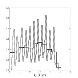
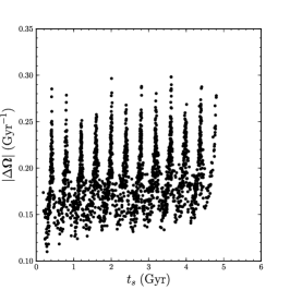
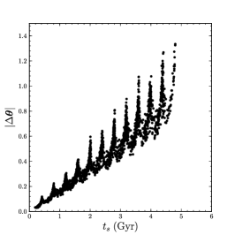
Figure 3.— Properties of the simulated tidal stream of $\mathsection$ 3.1 as a function of time. Stripping times are calculated by linear regression of the angle difference between a stream particle and the progenitor versus the equivalent frequency difference. The distribution of stripping times is shown in the left panel. While the stripping process happens in bursts with a period of roughly $400\,\mathrm{Myr}$ (the radial period of the progenitor), it can be approximated as constant (more coarsely-binned solid histogram). The magnitude of the frequency offset between stream particles and the progenitor is shown in the middle panel. While particles stripped at pericenter have larger frequency offsets than those between pericenter passages, there is almost no secular trend and the typical frequency offset (averaged over a radial period) can be considered constant with time. The right panel shows the magnitude of the angle offset between stream particles and the progenitor as a function of stripping time. There is a spread in the angle offset at all stripping times because of the dispersion in frequency offsets, but typically stars that have been stripped earlier reach larger angle offsets. That is, self-sorting happens only to a small degree.

Ingredients (a) and (b) require more careful modeling. The right panel of Figure 3 shows the distribution of times at which stream particles are stripped from the progenitor. These stripping times are calculated from the final snapshot by linear regression of a particle’s angle offset $\Delta\boldsymbol{\theta}$ from the progenitor, versus the frequency offset $\Delta\mathbf{\Omega}$ as

$$t_{s}=\frac{\Delta\mathbf{\Omega}\cdot\Delta\boldsymbol{\theta}}{|\Delta\mathbf{\Omega}|^{2}}\,.$$ (3)

The dotted line shows a finely-binned histogram of these stripping times, which indicates that stripping happens in bursts with a period of about $400\,\mathrm{Myr}$, the radial period of the progenitor’s orbit. Thus, as expected, stripping happens primarily at pericenter passages, with a smaller number of particles lost between pericenter passages. Realistic models of a stream, especially those that require good models of the surface-density structure of the stream as a function of stream angle, need to model this non-uniform stripping process. In what follows, we will use a uniform distribution of stripping times. This is appropriate for modeling the large-scale structure of streams, such as what is used when constraining the gravitational potential.

The middle panel of Figure 3 shows the frequency offsets between stream particles and the progenitor as a function of stripping time, corresponding to ingredient (b) above. The same burstiness that is apparent in the distribution of stripping times shows up here. Particles stripped at pericenter typically have larger frequency offsets than those lost at larger radii. This can be described as saying that particles are removed at pericenter, but only peeled off between pericenter passages. Again, realistic models of tidal streams need to take this detailed structure into account.

The right panel of Figure 3 shows the angle offset (at the end of the simulation) versus the stripping time. There is a spread in the angle offset reached for any given stripping time, but it is nevertheless typically the case that particles that have been stripped earlier are found at larger angle offsets today. Self-sorting—the tendency of particles stripped later with larger frequency offsets to overtake particles stripped earlier at smaller frequency differences and thus to erase correlations between particle position along the stream and stripping time and sort the stream in frequency offset—happens to a small extent but the narrow distribution of frequency offsets limits the ability of particles removed later to reach large distances from the progenitor.

We can model streams in frequency space because the mapping $\mathbf{J}\rightarrow\mathbf{\Omega}$ is of full rank for axisymmetric and triaxial potentials. However, for spherical potentials this mapping only has rank two, because $\Omega_{\phi}=\mathrm{sgn}(L_{Z})\,\Omega_{Z}$, such that the determinant $|\partial\mathbf{\Omega}/\partial\mathbf{J}|$ is zero. For spherical potentials, tidal streams only spread in a five-dimensional subspace and when modeling streams in spherical potentials we need to keep the direction perpendicular to this subspace constant.

3.3. The fiducial stream model

The discussion of the simulated stream’s properties as a function of stripping time in the previous section indicates that we can build simple models of the structure of tidal streams when considering them in frequency–angle space. In this section, I propose a very simple fiducial model that I will use in the remainder of this paper. This model combines simple analytic forms for ease of computation that are nevertheless realistic enough to provide adequate models for tidal streams in many applications.

First, we approximate the bursty, non-uniform distribution of stripping times in Figure 3 with a uniform distribution

$$\begin{split}p(t_{s})&\propto 1\,,\qquad 0<t_{s}<t_{d}\\ &=0\,,\qquad\mathrm{otherwise}\,.\end{split}$$ (4)

The thick, solid histogram in the right panel of Figure 3 shows a coarser-binned histogram of stripping times, indicating that the uniform distribution is a good approximation over intervals longer than a radial period ($\approx 400\,\mathrm{Myr}$). The disruption time $t_{d}$ is a free parameter of the model that needs to be determined for each stream. For the model of the simulated stream used here I set $t_{d}=4.5\,\mathrm{Gyr}$. This distribution of stripping times is different from that of Johnston (1998), who assumed that stripping happens exactly at pericenter and is therefore a sum of delta functions located at each pericenter passage. We do not consider such a distribution here further, but it should be straightforward to repeat the analytical calculations in $\mathsection$ 4 and 6 below for this alternative distribution.

Similarly, we model the distribution of frequency offsets between stream particles and the progenitor to be independent of stripping time, even though the middle panel of Figure 3 clearly shows that particles are stripped at larger frequency differences at pericentric passages than between them. The fact that there is only a small long-term trend in the typical frequency offset means that this is a good model on time-scales larger than the radial period. While this means that the small-scale structure of the stream will not be perfectly represented by the model, the large-scale structure of the stream will be fine. For using tidal streams to constrain the gravitational potential, large arcs are most important, such that this simple model will be adequate for such inferences.

The distribution of frequencies is three dimensional. Because we model the leading and the trailing arm separately, a single-peaked distribution suffices to describe the frequency distribution. A general description in terms of a Gaussian distribution would have nine free parameters. However, we can model it with fewer free parameters as follows. First, following Eyre & Binney (2011), we approximate the action distribution as a Gaussian with standard deviations given by the approximate spread in the actions $(\delta J_{R},\delta L_{Z},\delta J_{Z})$ in the cluster

$$\sigma_{J_{R}} \approx\delta\left(\frac{1}{2\,\pi}\oint\mathrm{d}r\,p_{r}\right)\approx\frac{1}{\pi}\,\sigma_{v}\,\left(r_{\mathrm{apo}}-r_{\mathrm{peri}}\right)\,,$$ (5)

$$\sigma_{L_{Z}} \approx\delta L_{Z}\approx\sigma_{v}\,r_{\mathrm{peri}}\,,$$ (6)

$$\sigma_{J_{Z}} \approx\delta\left(\frac{1}{\pi}\oint\mathrm{d}z\,p_{z}\right)\approx\frac{2}{\pi}\,\sigma_{v}\,Z_{\mathrm{max}}\,,$$ (7)

where $\sigma_{v}$ is the velocity dispersion of the progenitor, $r_{\mathrm{apo}}$ and $r_{\mathrm{peri}}$ are the apo- and pericenter radii of the progenitor orbit, respectively, and $Z_{\mathrm{max}}$ is the maximum $Z$ reached on this orbit. We assume that all of the correlations between the actions are zero (see Figure 2). Then we propagate this Gaussian variance to frequency space using the Hessian $(\partial\mathbf{\Omega}/\partial\mathbf{J})\large|_{\mathbf{J}^{p}}$, which gives the variance matrix $V_{\mathbf{\Omega}}$. The principal eigenvector of this matrix is the model direction along which the stream spreads. While the model I propose here is a simple one, it works well without having been tweaked for the simulation under scrutiny. The angle between the principal eigenvector of $V_{\mathbf{\Omega}}$ and the progenitor’s frequency vector is $0.50^{\circ}$ which is close to the value measured from the simulation using the mean frequency-offset vector is $0.18^{\circ}$ (see Figure 2). For a model with an isotropic action distribution, the misalignment would be $1.28^{\circ}$, much larger than the measured value.

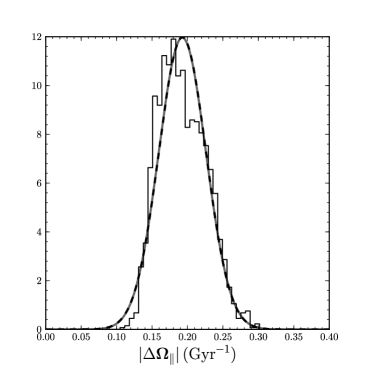
Figure 4.— Distribution of the magnitude of frequency offsets between stream particles and the progenitor along the direction of the mean frequency offset. The dashed line is a Gaussian fit to this distribution, while the solid line is a fit of our preferred form for this distribution, given in equation (8) (the dashed and solid lines almost entirely overlap). Both forms provide adequate fits to the distribution.

I then further constrain the mean frequency offset to lie along the principal eigenvector of $V_{\mathbf{\Omega}}$. Therefore, this mean frequency offset can be described in terms of a parameter $\mu_{\Omega}=\Delta\Omega^{m}/\sigma_{\Omega,1}$, where $\sigma_{\Omega,1}$ is the square root of the largest eigenvalue of $V_{\mathbf{\Omega}}$ and $\Delta\Omega^{m}$ is the one-dimensional mean frequency offset. The sign of $\mu_{\Omega}$ sets whether we are modeling a leading or a trailing arm. We can gain insight on good values for $\mu_{\Omega}$ from the simulation. Figure 4 shows the distribution of frequency offsets in the direction of the median frequency offset in the stream. Two fits to this distribution are displayed in Figure 4. The dashed line is a Gaussian fit to this distribution, while the solid line is a fit of the form

$$p(|\Delta\mathbf{\Omega}|_{\parallel})\propto|\Delta\mathbf{\Omega}|_{\parallel}\,\mathcal{N}\left(|\Delta\mathbf{\Omega}|_{\parallel}|\Delta\Omega^{m},\sigma_{\Omega,1}^{2}\right)\,,$$ (8)

where $\mathcal{N}(x|m,v)$ represents a Gaussian distribution for $x$ with mean $m$ and variance $v$. The fit is equally good (because the dispersion is much smaller than the mean) and I choose the second form because it simplifies some of the stream-track calculations below. The best-fit $(\Delta\Omega^{m},\sigma_{\Omega,1})$ is $(0.19,0.033)\,\mathrm{Gyr}^{-1}$ for both fits. Based on this information, a model with $\sigma_{v}=0.365\,\mathrm{km\ s}^{-1}$ and $\mu_{\Omega}=6$ provides a good fit to the simulation data. The distribution of frequency offsets in the two-dimensional space perpendicular to the principal eigenvector of $V_{\mathbf{\Omega}}$ is modeled as a zero-mean Gaussian with variance matrix given by the projection of $V_{\mathbf{\Omega}}$ onto this space.

Because we expect the typical $\Delta\mathbf{\Omega}$ to scale with the velocity dispersion of the progenitor, I conjecture that a constant $\mu_{\Omega}$ can be used for modeling tidal streams of any (small-ish) velocity dispersion. Further modeling of simulated streams, however, is necessary to check this and to find the optimal value of $\mu_{\Omega}$. In particular, if the progenitor has internal rotation the action distribution of the debris and $\mu_{\Omega}$ may be significantly different. Fixing $\mu_{\Omega}$ leaves a single free parameter $\sigma_{v}$ for modeling the frequency offset distribution of a tidal stream. In modeling observed data, this parameter needs to be fit and we expect it to be proportional to the velocity dispersion of the progenitor, although this proportionality needs to be checked more carefully. The discussion in $\mathsection$ 5 and Figure 3 in Sanders & Binney (2013a) demonstrates that the size of the frequency distribution scales as mass^1/3 over more than five orders of magnitude in mass, or approximately as the velocity dispersion through application of the virial theorem and the expression for the tidal radius as a function of the progenitor mass. Similarly, Johnston (1998) successfully modeled streams by assuming that the scale of the energy distribution in the stream is proportional to mass^1/3. The initial angle distribution, modeled here as an isotropic Gaussian, has a characteristic spread $\sigma_{\theta}$ which I set here to $\sigma_{\theta}=0.003$ ($=\sigma_{v}/[122\,\mathrm{km\ s}^{-1}]$) for the model $\sigma_{v}=0.365\,\mathrm{km\ s}^{-1}$; see above) based on a comparison with the simulation data, and we likewise expect this spread to scale with the velocity dispersion of the progenitor.

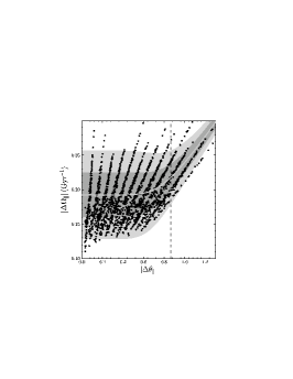
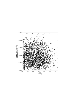
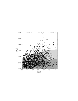
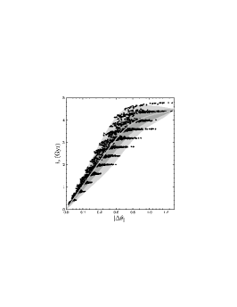
Figure 5.— Stream properties as a function of angle along the stream. The top, left panel shows the magnitude of frequency offsets along the stream. The gray line shows the mean predicted frequency offset calculated using the framework of $\mathsection$$\mathsection$ 3.2 and 4, while the grayscale bands show the $68\,\%$ and $95\,\%$ limits of the predicted distribution. The dashed line shows the angle $\theta_{\parallel}=\Delta\Omega^{m}\,t_{d}$, angles beyond which can only be reached by having a larger $\Delta\Omega_{\parallel}$ than average. The top, right panel shows the magnitude of frequency offsets perpendicular to those in the left panel. The predicted distribution is constant as a function of angle and therefore not shown. The bottom, left panel shows the angle offset perpendicular to the stream and the grayscale bands show $68\,\%$ and $95\,\%$ limits of the predicted distribution of angle offsets; the white dashed line shows the $68\,\%$ limit calculated using a simplified method. The bottom, right panel shows the stripping time. The gray line and grayscale bands again show the mean and $68\,\%$ and $95\,\%$ confidence limits of the predicted distribution. While the “burstiness” related to the energetic stripping at pericenter that is apparent in the simulated data’s distributions is (by design) absent in the model, the overall scale and the mean trends with angle are well represented by the model.

The fiducial model for a tidal stream in frequency–angle coordinates proposed here is therefore described by essentially two free parameters in addition to the progenitor’s phase-space position: the progenitor’s velocity dispersion $\sigma_{v}$ and the disruption time $t_{d}$. As shown below, these two parameters are the most important in determining the track of the stream. More sophisticated models can leave $\mu_{\Omega}$ and $\sigma_{\theta}$ as free parameters as well. In what follows, I will fix these to the values given in the previous paragraphs. It must be stressed, however, that all of these parameters here have been fixed “by-eye”, and better fits might be possible using more quantitative fit procedures.

4. The track of a tidal stream

In this Section, I discuss how to calculate the track of a model tidal stream in the generative model described in $\mathsection$ 3. The track consists of the mean location of the stream as a function of angle along the stream. I also describe how to estimate the dispersion of the stream along this track. In $\mathsection$ 4.1, I explain how to calculate the track of the stream in frequency–angle coordinates as well as how to estimate the spread around this track. In $\mathsection$ 4.2 I discuss how to efficiently project the stream track and dispersion into position–velocity coordinates $(\mathbf{x},\mathbf{v})$ or observable coordinates $(l,b,D,V_{\mathrm{los}},\mu_{l},\mu_{b})$.

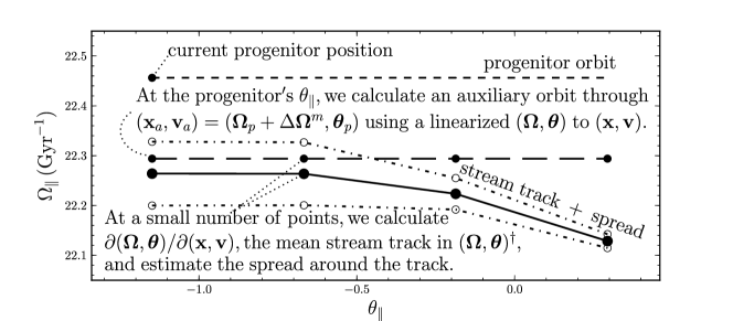
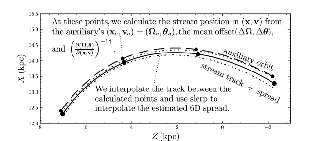
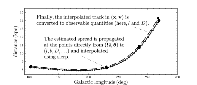
Figure 6.— Illustration of the determination of the average stream track described in $\mathsection$ 4. The small black dots in each panel are the points along the auxiliary orbit at which the Jacobian $\partial(\mathbf{\Omega},\boldsymbol{\theta})/\partial(\mathbf{x},\mathbf{v})$ is calculated. The large black dots are the corresponding points on the stream where the track is calculated. The short-dashed line in each panel is the progenitor’s orbit, the long-dashed line is the auxiliary orbit, and the solid line and dash-dotted lines are the mean track and $2\sigma$ dispersion. The daggers ($\dagger$) indicates the step in this procedure where the calculation of the mean stream track in $(\mathbf{x},\mathbf{v})$ can be iterated (see text). The offset between the auxiliary orbit and the stream track is exaggerated for display purposes in all panels; typically the auxiliary orbit is very close to the stream track.

4.1. In frequency–angle coordinates

In the generative model described above, the direction of the angle along the stream lies along the principal eigenvector of $V_{\mathbf{\Omega}}$, the variance matrix of the model $\Delta\mathbf{\Omega}$ distribution. We denote the angle in this direction as $\theta_{\parallel}$ and the frequency in this direction $\Omega_{\parallel}$; the two-dimensional angle- and frequency-space perpendicular to this direction is denoted as $\boldsymbol{\theta}_{\perp}$ and $\mathbf{\Omega}_{\perp}$.

First, we compute the distribution of $\Delta\Omega_{\parallel}$, the frequency offset between stream members and the progenitor given the angle offset $\Delta\theta_{\parallel}$ as follows (considering $\Delta\Omega_{\parallel}$ to be positive)

$$\begin{split}p(\Delta\Omega_{\parallel}|\Delta\theta_{\parallel})&=\int\mathrm{d}t_{s}\,p(\Delta\Omega_{\parallel},t_{s}|\Delta\theta_{\parallel})\,\\ &\propto\int\mathrm{d}t_{s}\,p(\Delta\theta_{\parallel}|\Delta\Omega_{\parallel},t_{s})\,p(\Delta\Omega_{\parallel},t_{s})\,,\\ &\approx\int\mathrm{d}t_{s}\,\delta(\Delta\theta_{\parallel}-\Delta\Omega_{\parallel}\,t_{s})\,p(\Delta\Omega_{\parallel},t_{s})\,,\\ &=\frac{1}{\Delta\Omega_{\parallel}}\,p(\Delta\Omega_{\parallel},\frac{\Delta\theta_{\parallel}}{\Delta\Omega_{\parallel}})\,,\end{split}$$ (9)

where in the penultimate step I have approximated the initial angle distribution as a delta function (as the initial angle offset is small with respect to the final offset). This is a fully general expression. For the fiducial stream model, this can be simplified to

$$\begin{split}p(\Delta\Omega_{\parallel}|\Delta\theta_{\parallel})\propto&\ \frac{1}{\Delta\Omega_{\parallel}}\,p(\Delta\Omega_{\parallel})\,,\qquad 0<\frac{\Delta\theta_{\parallel}}{\Delta\Omega_{\parallel}}<t_{d}\,.\\ &0\,,\qquad\mathrm{otherwise}\,.\end{split}$$ (10)

Equation (10) shows why I chose to model $p(\Delta\Omega_{\parallel})$ as a Gaussian multiplied with $|\Delta\Omega_{\parallel}|$. $p(\Delta\Omega_{\parallel}|\Delta\theta_{\parallel})$ is then a Gaussian with mean $\Delta\Omega^{m}$ and variance $\sigma^{2}_{\Omega,1}$, for $\Delta\Omega_{\parallel}>\Delta\theta_{\parallel}/t_{d}$, and zero otherwise. The mean and variance of such a Gaussian is straightforward to calculate in terms of error functions. The top left panel of Figure 5 shows the distribution of $|\Delta\Omega_{\parallel}|$ versus $|\Delta\theta_{\parallel}|$ (absolute value in order to show the trailing and leading stream together) for the simulated stream, as well as the mean and dispersion calculated from the fiducial model. The dashed line shows $\Delta\theta_{\parallel}=\Delta\Omega^{m}\,t_{d}$, approximately the angle where the finite disruption time starts to influence the mean $\Delta\Omega_{\parallel}$ of the stream. The finite disruption time, $\approx 4.5\,\mathrm{Gyr}$ in this case, of a tidal stream means that for stream members to have reached very large angle differences with respect to the progenitor, they must have been removed at large frequency differences. Around $\Delta\Omega^{m}\,t_{d}$, average stream stars, i.e., those removed with the average frequency offset, do not have a large enough offset to reach large angle offsets. Therefore, even though the average frequency offset does not change much over time (see Figure 3), the average frequency offset, and therefore the average orbit, does change with distance from the progenitor.

In the fiducial model, the average $\Delta\mathbf{\Omega}_{\perp}$, and $\Delta\boldsymbol{\theta}_{\perp}$ as a function of $\Delta\theta_{\parallel}$ are zero. Therefore, the average stream track as a function of $\Delta\theta_{\parallel}$ is entirely specified by the mean $\Delta\Omega_{\parallel}(\Delta\theta_{\parallel})$ in the parallel direction and zero offsets in the perpendicular directions. This track can be rotated into the $(R,\phi,Z)$ coordinate system using the eigenvectors of $V_{\mathbf{\Omega}}$.

To estimate the spread around the stream track, we need to calculate the distributions $p(\Delta\mathbf{\Omega}_{\perp}|\Delta\theta_{\parallel})$ and $p(\Delta\boldsymbol{\theta}_{\perp}|\Delta\theta_{\parallel})$. The former is just the zero mean Gaussian with variance given by the projection of $V_{\mathbf{\Omega}}$ onto the direction perpendicular to the stream. The distribution $p(\Delta\boldsymbol{\theta}_{\perp}|\Delta\theta_{\parallel})$, however, does depend on $\Delta\theta_{\parallel}$, because $\Delta\boldsymbol{\theta}_{\perp}=\Delta\boldsymbol{\theta}_{\perp}^{\mathrm{init}}+\Delta\mathbf{\Omega}_{\perp}t_{s}$ and the distribution of $t_{s}$ depends on $\Delta\theta_{\parallel}$. Therefore, we first calculate $p(t_{s}|\Delta\theta_{\parallel})$.

We can calculate $p(t_{s}|\Delta\theta_{\parallel})$ as follows

$$\begin{split}p(t_{s}|\Delta\theta_{\parallel})&=\int\mathrm{d}\Delta\Omega_{\parallel}\,p(t_{s},\Delta\Omega_{\parallel}|\Delta\theta_{\parallel})\,,\\ &=\int\mathrm{d}\Delta\Omega_{\parallel}\,p(t_{s}|\Delta\Omega_{\parallel},\Delta\theta_{\parallel})\,p(\Delta\Omega_{\parallel}|\Delta\theta_{\parallel})\,,\\ &\approx p\left(\Delta\Omega_{\parallel}=\frac{\Delta\theta_{\parallel}}{t_{s}}\right)\,\left|\frac{\Delta\theta_{\parallel}}{(t_{s})^{2}}\right|\,,\end{split}$$ (11)

where in the last step I have again approximated the initial distribution of parallel angle offsets as a delta function. The first factor in this equation is given by the expression given in equation (9) (in general) or in equation (10) for the fiducial model. The lower right panel of Figure 5 shows the distribution of stripping times for members of the simulated stream as well as the mean and dispersion calculated from equation (11). Similar to the distribution of $\Delta\Omega_{\parallel}$ as a function of $\Delta\theta_{\parallel}$, the distribution of $t_{s}$ has a kink at the angle offset that can only be reached by stars that have to have been stripped at large frequency offsets (that is, larger than average).

We can now also calculate $p(\Delta\boldsymbol{\theta}_{\perp}|\Delta\theta_{\parallel})$:

$$\begin{split}p(\Delta\theta_{\perp,ii}|\Delta\theta_{\parallel})&=\int\mathrm{d}t_{s}\,\mathrm{d}\Delta\Omega_{\perp,ii}\,p(\Delta\theta_{\perp,ii}|\Delta\Omega_{\perp,ii},t_{s})\\ &\qquad\times p(\Delta\Omega_{\perp,ii}|t_{s},\Delta\theta_{\parallel})\,p(t_{s}|\Delta\theta_{\parallel})\,,\end{split}$$ (12)

where $ii=2,3$ for the first and second perpendicular direction. For the fiducial model, this simplifies to

$$\begin{split}p(\Delta\theta_{\perp,ii}|\Delta\theta_{\parallel})&=\int\mathrm{d}t_{s}\,\mathcal{N}\left(\Delta\theta_{\perp,ii}|0,\sigma_{\theta}^{2}+(t_{s}\,\sigma_{\Omega,ii})^{2}\right)\qquad\\ &\qquad\times p(t_{s}|\Delta\theta_{\parallel})\,,\end{split}$$ (13)

where $\sigma_{\Omega,ii}$ is the model frequency dispersion in the perpendicular direction (corresponding to the middle and smallest eigenvalue of $V_{\mathbf{\Omega}}$). I have not approximated the initial angle-offset distribution as a delta function here, because its width is a significant fraction of that of the final perpendicular-angle-offset distribution. In the fiducial model, this distribution is the only one of those considered in this section that requires an explicit integration. However, we can approximate the distribution by using the mean $t_{s}(\Delta\theta_{\parallel})$ rather than integrating over $t_{s}$. The lower left panel of Figure 5 shows the distribution of perpendicular angle offsets and the grayscale bands show the dispersion calculated using equation (13); the white dashed line shows the approximate estimate obtained using the mean stripping time rather than integrating over it. This simple estimate agrees well with the exact calculation.

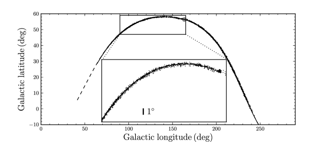
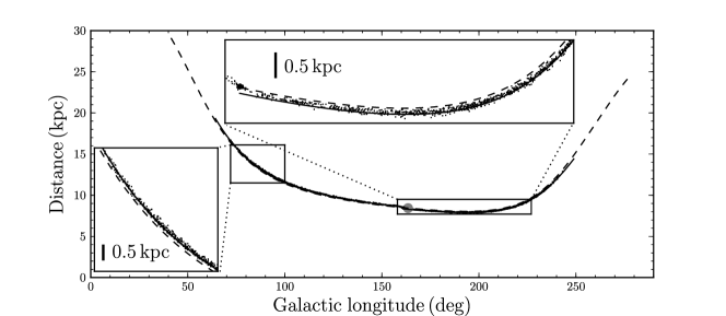
Figure 7.— Simulated stream after $5.011\,\mathrm{Gyr}$ as a function of Galactic longitude. The top panel shows the stream in Galactic latitude and the bottom panel shows it in the distance from the Sun. The progenitor is shown as the large gray dot and its orbit as the dashed lines. The predicted track of the stream is shown as the solid line. Insets show various zoomed-in parts of the stream to show the stream, progenitor orbit, and predicted stream track up close.

We can then estimate the dispersion around the stream track, which is useful for getting a sense of the width of the model stream and to find appropriate integration intervals when marginalizing the stream PDF as discussed in $\mathsection$ 6. At a given angle offset $\Delta\theta_{\parallel}$ we calculate the dispersion in $\Delta\Omega_{\parallel}$ from equation (10) and we substitute this appropriately in $V_{\mathbf{\Omega}}$. We can also calculate the dispersion in $\Delta\boldsymbol{\theta}_{\perp}$ using equation (13). How to estimate the dispersion in $\Delta\theta_{\parallel}$ near a given $\Delta\theta_{\parallel}$ is more difficult, and I simply use a dispersion of $1$, as the stream typically spreads out over $\approx 1$ radian. We could calculate the correlation between $\Delta\Omega_{\perp,ii}$ and $\Delta\theta_{\perp,ii}$ using similar equations as those given in the previous paragraphs, but for a simple estimate we can approximate these as $0.5$; I set the correlation between $\Delta\Omega_{\parallel}$ and $\Delta\theta_{\parallel}$ to zero. While these estimates are not perfect, they give a reasonable estimate of the dispersion along the stream track. This provides an adequate starting point for more precise calculations of the dispersion in $\mathsection$ 6.

4.2. In position–velocity coordinates

Having estimated the track of the stream and the dispersion around this in frequency–angle space, we can propagate the track to position–velocity coordinates by inverting the transformation $(\mathbf{x},\mathbf{v})\rightarrow(\mathbf{\Omega},\boldsymbol{\theta})$. I do this by linearizing the transformation in the vicinity of the stream along an estimate of the stream track, obtained using the procedure below, and inverting this linearized transformation. That this works relies on the stream being relatively cold (in that $\sigma_{v}/V_{c}\ll 1$) for a few different reasons. First, the track of a cold stream, while in general offset from the orbit of the progenitor, does not stray too far from it close to the progenitor, such that the transformation to frequency–angle coordinates can be linearized over the range of the stream–orbit offset close to the progenitor. Second, cold streams are essentially one-dimensional, that is, they only spread significantly over a single direction. This means that non-linearity in the $(\mathbf{x},\mathbf{v})\rightarrow(\mathbf{\Omega},\boldsymbol{\theta})$ transformation only affects a single direction. Therefore, we can linearize the $(\mathbf{x},\mathbf{v})\rightarrow(\mathbf{\Omega},\boldsymbol{\theta})$ transformation along a one-dimensional grid of points, rather than on a full six-dimensional grid. Third, the coldness of the stream means that any significant mass of the full stream PDF is close enough to the stream track that all frequency–angle calculations can be performed using the linear approximation along the progenitor orbit.

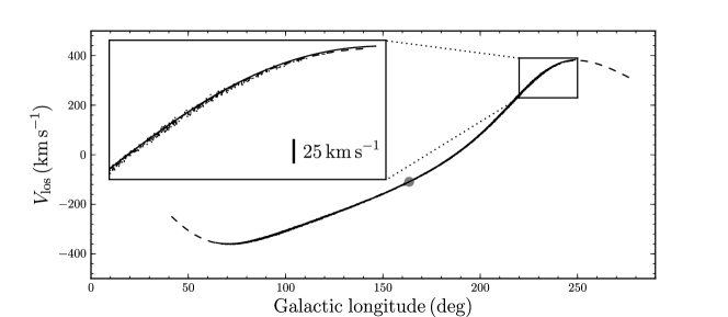
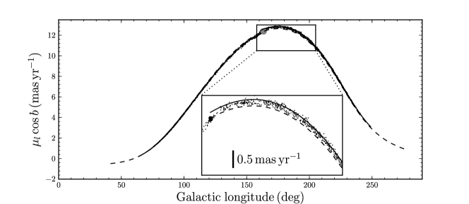
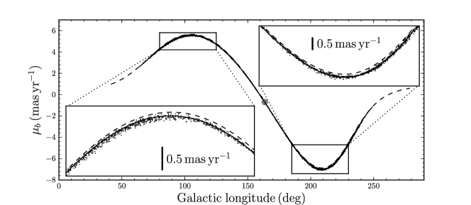
Figure 8.— Simulated stream velocities as a function of Galactic longitude. Same as Figure 7, but for the stream in heliocentric line-of-sight velocity $V_{\mathrm{los}}$ (top panel), proper motion in the direction of Galactic longitude (middle panel), and in the direction of Galactic latitude (bottom panel). Insets again show various interesting parts of the stream up close.

Figure 6 illustrates how I linearize the $(\mathbf{x},\mathbf{v})\rightarrow(\mathbf{\Omega},\boldsymbol{\theta})$ transformation and use it to propagate the track of the stream to position–velocity coordinates and to observable quantities $(l,b,D,V_{\mathrm{los}},\mu_{l},\mu_{b})$. The top panel shows the orbit of the progenitor, an auxiliary orbit, and the mean stream track in frequency–angle coordinates. Only the projection onto the parallel direction is shown here. The auxiliary orbit is determined by converting the mean stream frequency $\mathbf{\Omega}=\mathbf{\Omega}_{p}+\Delta\mathbf{\Omega}$, where $\Delta\mathbf{\Omega}$ is determined using the techniques from the previous section, at zero angle difference with respect to the progenitor to $(\mathbf{x},\mathbf{v})$ and integrating this orbit. The transformation to configuration space is done by linearizing the $(\mathbf{x},\mathbf{v})\rightarrow(\mathbf{\Omega},\boldsymbol{\theta})$ transformation around $(\mathbf{x}_{p},\mathbf{v}_{p})$ and inverting this transformation. At a small number of points along the auxiliary orbit, chosen here to span $1.5$ radians, we calculate the Jacobian $\partial(\mathbf{\Omega},\boldsymbol{\theta})/\partial(\mathbf{x},\mathbf{v})$. In this Figure this is done at four points, but for all other figures and calculations in this paper eleven points are used. Each Jacobian calculation requires seven frequency–angle calculations, such that the total number of such computations is less than $100$ to adequately model the stream (each computation involves a single orbit integration, see Appendix A).

We then calculate the stream track in Galactocentric position–velocity coordinates at the parallel angles for which we have linearized the frequency–angle transformation. This is shown in the middle panel of Figure 6. Similarly, we transform the approximated variance described at the end of the previous section to position–velocity coordinates under the linear approximation. We can then interpolate the track of the stream between this small number of points at which it is calculated; this gives the full track of the stream. In $\mathsection$ 6, we require an estimate of the dispersion around the track at any angle along the stream (for calculating the marginalized PDF). We can obtain this from interpolating the estimated variances at the calculated track points. This interpolation can be performed practically as follows. We decompose the variance matrix at each calculated track point into its eigendecomposition and order the eigenvalues by size. We then interpolate each of the six eigenvalues using spline interpolation. The direction of each eigenvector is interpolated using slerp (Shoemake, 1985), which is a type of spherical linear interpolation. The variance matrix at interpolated track points can then be constructed from the interpolated eigenvalues and eigenvectors. All other $(\mathbf{x},\mathbf{v})\leftrightarrow(\mathbf{\Omega},\boldsymbol{\theta})$ calculations can then be performed by using the closest interpolated track point in $(\mathbf{x},\mathbf{v})$ or $(\mathbf{\Omega},\boldsymbol{\theta})$ and using the calculated Jacobian from the closest calculated track point.

Finally, we can calculate the stream track in observable quantities $(l,b,D,V_{\mathrm{los}},\mu_{l},\mu_{b})$ by converting the interpolated track in $(\mathbf{x},\mathbf{v})$ to these coordinates. The dispersion at calculated track points is calculated from that in $(\mathbf{\Omega},\boldsymbol{\theta})$ using the appropriate Jacobians and the six-dimensional dispersion can again be interpolated using the eigendecomposition. This is illustrated in the bottom panel of Figure 6.

This procedure for propagating the stream track from frequency–angle space to configuration space works well when the misalignment between the stream track and a single orbit is not too large (as is the case for the example used throughout in this paper). However, when this misalignment is large, the auxiliary orbit deviates significantly from the stream track and the linear approximations to go from auxiliary orbit to stream track break down. This can be diagnosed by calculating the frequencies and angles along the estimated stream track in configuration space using the algorithm in Appendix A and comparing it to those of the desired stream track computed using the methods from the previous section. When the misalignment is large and the linear approximations break down, these two do not agree (in that they deviate by much more than the spread in the stream around the mean track).

We can fix this by iterating the calculation of the stream track. After the first estimate of the stream track is obtained using the auxiliary orbit, we can compute another estimate starting from the previous estimate of the stream track—now the auxiliary track, because it is no longer a single orbit—in $(\mathbf{x},\mathbf{v})$ in the same way as the first estimate was calculated. Thus, we linearize the $(\mathbf{x},\mathbf{v})\rightarrow(\mathbf{\Omega},\boldsymbol{\theta})$ transformation around points along the auxiliary track and calculate a new estimate of the stream track based on the offset in frequency–angle between the auxiliary track and the desired track. Even for large misalignments, this procedure converges in a few iterations (that is, the difference between the calculated stream track and the desired stream track in frequency–angle becomes much smaller than the dispersion within the stream).

The average stream location computed in the manner described in this section is an approximate track. The mean stream location, for example, in distance from the Sun at a given Galactic longitude, can be exactly calculated by marginalizing over the full six-dimensional stream PDF in $(l,b,D,V_{\mathrm{los}},\mu_{l},\mu_{b})$ over the unobserved dimensions $(b,V_{\mathrm{los}},\mu_{l},\mu_{b})$. In general this will give a slightly different stream location, because the stream DF is not exactly Gaussian. However, it is demonstrated in $\mathsection$ 6, where I calculate the full stream PDF, that the approximate mean stream location of this section is sufficiently close to the true average position for all practical purposes. The same should hold for any cold stream.

Figure 1 shows the simulated stream particles as well as the stream track calculated in this section in Galactocentric $X$ and $Z$ coordinates. It is clear that the average stream location tracks the position of the simulated stream. Figures 7 and 8 show the same, but in observed coordinates $(l,b,D,V_{\mathrm{los}},\mu_{l},\mu_{b})$. These figures show that the simple fiducial stream model does a good job of predicting where the stream is located as a function of Galactic longitude.

5. Mock stream data

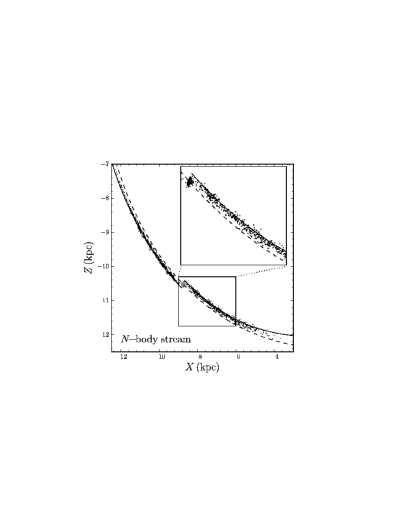
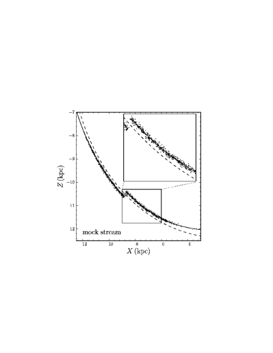
Figure 9.— Mock stream data generated from the model. The top panel shows the same $N$-body stream as shown in previous figures, but $1.96\,\mathrm{Gyr}$ earlier in its evolution. Symbols, lines, and the stream model are the same as those in Figure 1, except that the model progenitor phase-space location from Figure 1 has been integrated backward in time for $1.96\,\mathrm{Gyr}$ and the model disruption time was reduced by $1.96\,\mathrm{Gyr}$ (no other changes were made to the model’s parameters). The bottom panel shows mock stream data drawn from the model using the procedures discussed in $\mathsection$ 5. The gap between the leading and the trailing arm is due to the difference in mean frequency between the arms. Overall, the spatial distribution of the mock data is very similar to that of the $N$-body stream.

Using the generative model described in $\mathsection$ 3.2, it is straightforward to draw mock stream data in frequency–angle space. The three ingredients—time, frequency, and angle distributions of the debris—allow for mock data to be generated in four steps. First, a stripping time $t_{s}$ is sampled from the distribution of stripping times. Second, a frequency offset $\Delta\mathbf{\Omega}$ with respect to the progenitor is drawn from the frequency distribution at $t_{s}$. Third, an initial angle offset is drawn. Fourth, the initial angle offset is incremented by $\Delta\mathbf{\Omega}\,t_{s}$. This generates the final frequency–angle coordinates of the mock stream member $(\Delta\mathbf{\Omega},\Delta\boldsymbol{\theta}+\Delta\mathbf{\Omega}\,t_{s})+(\mathbf{\Omega}_{p},\boldsymbol{\theta}_{p})$.

For the fiducial stream model of $\mathsection$ 3.3 the procedure for producing mock data is simplified to sampling a small number of easy-to-sample distributions. First, $t_{s}$ is drawn uniformly between $0$ and $t_{d}$. Second, $\Delta\mathbf{\Omega}_{\perp}$ is drawn from the Gaussian distribution of $\Delta\mathbf{\Omega}_{\perp}$. The distribution of $\Delta\Omega_{\parallel}$ is not Gaussian, as it is a Gaussian in $|\Delta\Omega_{\parallel}|$ multiplied with $|\Delta\Omega_{\parallel}|$ over the range $\Delta\Omega_{\parallel}>0$. This distribution is log-concave, that is, the derivative of its logarithm is negative everywhere, and therefore it can be efficiently sampled using adaptive-rejection sampling (Gilks & Wild, 1992). The sign of $\Delta\Omega_{\parallel}$ is determined by whether we are generating a leading or trailing stream. Third, initial angle offsets are drawn from the Gaussian distribution of such offsets. The fourth step is as above.

To transform the mock stream in frequency–angle coordinates to position–velocity space, we use the approximate procedure for this transformation along the stream track described at the end of the previous section. The mock stream in $(\mathbf{x},\mathbf{v})$ can then be further transformed to observable coordinates $(l,b,D,V_{\mathrm{los}},\mu_{l},\mu_{b})$ or any other similar quantities as desired.

Figure 9 shows mock data generated for the model of the simulated stream described in $\mathsection$ 3.3. The mock data in this Figure have been generated $1.96\,\mathrm{Gyr}$ before the final snapshot of the simulation (that is, $1.96\,\mathrm{Gyr}$ before Figure 1). The model from $\mathsection$ 3.3, which was for the final snapshot, was adjusted to this earlier time by backward orbit integration of the model progenitor and by revising the disruption time downward by $1.96\,\mathrm{Gyr}$. No other changes were made to the model. The bottom panel of Figure 9 shows the mock data generated from the model in $(X,Z)$, while the top panel shows the simulated stream data at this time. Overall, the distribution of the mock and simulated data are similar.

6. The full stream PDF

Data on tidal streams typically come in one of two flavors: data on individual stream members, often with multiple missing phase–space components, or data describing the mean position and width of the stream. For the proper analysis of these kinds of data it is useful to be able to evaluate the PDF for the stream model described in this paper and to marginalize over or condition it on certain dimensions.

The generative model described in $\mathsection$ 3.2 corresponds to the stream PDF in frequency $\mathbf{\Omega}$, angle $\boldsymbol{\theta}$, and stripping time $t_{s}$

$$p(\mathbf{\Omega},\boldsymbol{\theta},t_{s})=p(t_{s})\,p(\mathbf{\Omega}|t_{s})\,p(\boldsymbol{\theta}|\mathbf{\Omega},t_{s})\,,$$ (14)

where the three factors on the right are specified through the three ingredients of $\mathsection$ 3.2. The PDF in position–velocity space is then given by

$$p(\mathbf{x},\mathbf{v},t_{s})=p(\mathbf{\Omega},\boldsymbol{\theta},t_{s})\,\left|\frac{\partial\mathbf{\Omega}}{\partial\mathbf{J}}\right|\,,$$ (15)

where $|\partial\mathbf{\Omega}/\partial\mathbf{J}|$ is equal to the Jacobian $|\partial(\mathbf{\Omega},\boldsymbol{\theta})/\partial(\mathbf{x},\mathbf{v})|$ because $|\partial(\mathbf{J},\boldsymbol{\theta})/\partial(\mathbf{x},\mathbf{v})|=1$. The PDF in observable quantities $(l,b,D,V_{\mathrm{los}},\mu_{l},\mu_{b})$ can be obtained from $p(\mathbf{x},\mathbf{v},t_{s})$ by multiplying by the Jacobian $\left|\partial(\mathbf{x},\mathbf{v})/\partial(l,b,D,V_{\mathrm{los}},\mu_{l},\mu_{b})\right|$.

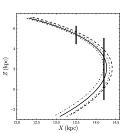
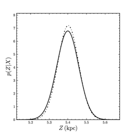
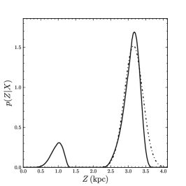
Figure 10.— Marginalized, conditional $p(Z|X)$ PDFs. The left panel shows the model leading stream (see Figure 1), with the stream track shown as the solid line, the estimated $2\sigma$ width of the stream as the dash-dotted line, and the progenitor orbit as the dashed line. The solid line in the middle and right panels shows $p(Z|X)$ calculated at the $X$ indicated in the left panel by thick vertical lines; the dash-dotted line is a simple Gaussian estimate. The upper branch near $Z\approx 5\,\mathrm{kpc}$ of the stream is chosen for the middle panel. The right panel shows an $X$ close to where the stream turns around in $X$; the PDF has multiple peaks in this case.

The stripping time $t_{s}$ cannot be observed and should therefore be marginalized over when evaluating the PDF. One of the great advantages of modeling a stream in frequency–angle coordinates is that this marginalization can be calculated analytically for many choices of $p(t_{s})$ if $p(\mathbf{\Omega}|t_{s})\equiv p(\mathbf{\Omega})$. Specifically, for the fiducial model $p(t_{s})$ is uniform up to a maximum disruption time $t_{d}$ (see equation [4]) such that we can write

$$\begin{split}p(&\mathbf{\Omega},\boldsymbol{\theta})\\ &=\int\mathrm{d}t_{s}\,p(\mathbf{\Omega},\boldsymbol{\theta},t_{s})\,,\\ &=p(\mathbf{\Omega})\,\int_{0}^{t_{d}}\mathrm{d}t_{s}\,\frac{1}{(2\,\pi)^{3/2}\,\sigma_{\theta}^{3}}\\ &\qquad\qquad\times\exp\left(-\frac{1}{2\,\sigma_{\theta}^{2}}\left[\sum_{R,\phi,Z}\left(\Delta\boldsymbol{\theta}_{i}-\Delta\mathbf{\Omega}_{i}\,t_{s}\right)^{2}\right]\right)\,,\end{split}$$ (16)

where the sum in the argument of the exponential is over the three components of $\Delta\boldsymbol{\theta}_{i}$ and $\Delta\mathbf{\Omega}_{i}$. This integral can be done analytically, resulting in

$$\begin{split}p(&\mathbf{\Omega},\boldsymbol{\theta})=p(\mathbf{\Omega})\,\frac{\mathrm{erf}(a_{0})+\mathrm{erf}(a_{d})}{4\,\pi\,\sigma_{\theta}^{2}\,|\Delta\mathbf{\Omega}|}\\ &\ \times\exp\left(-\frac{1}{2\,\sigma_{\theta}^{2}}\left[\sum_{R,\phi,Z}\Delta\boldsymbol{\theta}^{2}_{i}-\frac{\left(\sum_{R,\phi,Z}\Delta\mathbf{\Omega}_{i}\Delta\boldsymbol{\theta}_{i}\right)^{2}}{|\Delta\mathbf{\Omega}|^{2}}\right]\right)\,.\end{split}$$ (17)

In this expression, $\Delta X^{2}\equiv(X_{1}-X_{2})^{2}$. The expression in square brackets is positive by using the Cauchy-Schwarz inequality. The quantities $a_{0}$ and $a_{d}$ in this expression are defined by the following expressions

$$\tilde{t}_{s} =\frac{\sum\Delta\mathbf{\Omega}_{i}\Delta\boldsymbol{\theta}_{i}}{|\Delta\mathbf{\Omega}|^{2}}\,,$$ (18)

$$a_{0} =\frac{|\Delta\mathbf{\Omega}|}{\sqrt{2}\,\sigma_{\theta}}\,\tilde{t}_{s}\,,$$ (19)

$$a_{d} =\frac{|\Delta\mathbf{\Omega}|}{\sqrt{2}\,\sigma_{\theta}}\,\left(t_{d}-\tilde{t}_{s}\right)\,.$$ (20)

The time $\tilde{t}_{s}$ is the best estimate of the stripping time for a given $\Delta\mathbf{\Omega}$ and $\Delta\boldsymbol{\theta}$. The quantity $a_{0}$ then serves to suppress the PDF in case the stripping time is smaller than zero, i.e., a stream member appears to have been removed in the future; in this case $\mathrm{erf}(a_{0})\approx-1$ and the PDF goes to zero. Similarly, $a_{d}$ suppresses the PDF when the stripping time is larger than $t_{d}$, i.e., the stream member seems to have been stripped before disruption began. Both of these get a tolerance corresponding to the initial angle spread. For example, if $\tilde{t}_{s}$ is negative, but so small such that $|\Delta\mathbf{\Omega}|\,\tilde{t}_{s}\sim\sigma_{\theta}$, the PDF is only mildly suppressed. For stars well within the stream $\mathrm{erf}(a_{0})+\mathrm{erf}(a_{d})\approx 2$.

We can marginalize equation (15) over $t_{s}$ and find that

$$p(\mathbf{x},\mathbf{v})=p(\mathbf{\Omega},\boldsymbol{\theta})\,\left|\frac{\partial\mathbf{\Omega}}{\partial\mathbf{J}}\right|\,.$$ (21)

When evaluating this PDF as a function of $(\mathbf{x},\mathbf{v})$ or as a function of observable quantities $(l,b,D,V_{\mathrm{los}},\mu_{l},\mu_{b})$ we calculate frequencies and angles using the approximate, linear transformation near the stream track as described at the end of $\mathsection$ 4.2. Thus, $p(\mathbf{x},\mathbf{v})$ can be evaluated very quickly by making efficient use of array operations. In this approximation the Jacobian $|\partial\mathbf{\Omega}/\partial\mathbf{J}|$ is constant everywhere near the track (for a given potential).

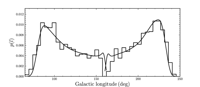
Figure 11.— Density distribution as a function of Galactic longitude. The smooth solid line shows the fiducial model’s prediction, while the histogram shows the density along the simulated stream. The simple fiducial stream model can accurately predict the density distribution along the stream.

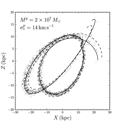
Figure 12.— Same as Figure 1, but for a simulation of a progenitor with a mass $M^{p}$ that is $1,000$ times larger and therefore a velocity dispersion $\sigma_{v}^{p}$ that is ten times larger. The model used to predict the stream track (solid line) is the same as that used in Figure 1, except that the model velocity dispersion $\sigma_{v}$ has been increased by a factor of ten. The stream spreads over a much larger volume for a heavier progenitor, but the fiducial model still accurately predicts its location in phase space.

We can marginalize the PDF over unobserved directions, convolve it with uncertainty distributions, or condition it on certain directions using the standard rules of probability theory; I will refer to all of these as marginalizations in what follows, as they all involve integrations over the PDF. In practice, to perform these marginalizations it is useful to estimate the extent of the PDF to define appropriate intervals for efficient numerical integration. For this we can use the average stream track and dispersion around it as estimated in $\mathsection$ 4. This is most easily explained through an example. To determine $p(Z|X)$, the distribution of Galactocentric $Z$ at a given Galactocentric $X$, we need to calculate

$$p(Z|X)=\frac{p(Z,X)}{p(X)}=\frac{\int\mathrm{d}Y\,\mathrm{d}\mathbf{v}\,p(\mathbf{x},\mathbf{v})}{\int\mathrm{d}Y\,\mathrm{d}Z\,\mathrm{d}\mathbf{v}\,p(\mathbf{x},\mathbf{v})}\,.$$ (22)

Thus, we need to marginalize over $(Y,\mathbf{v})$ in the numerator and $(Y,Z,\mathbf{v})$ in the denominator. Focusing on the numerator, we find the closest point on the stream track calculated as in $\mathsection$ 4.2 and calculate its six-dimensional Gaussian approximation. Then we condition this six-dimensional Gaussian on $(X,Z)$ using the standard rules of Gaussian conditioning (e.g., Appendix B of arXiv version 1 of Bovy et al. 2011) to obtain the approximate PDF $p(Y,\mathbf{v}|X,Z)$. We then evaluate $\int\mathrm{d}Y\,\mathrm{d}\mathbf{v}\,p(\mathbf{x},\mathbf{v})$ by numerical integration over the, e.g., $3\sigma$ range of this Gaussian; this numerical integration can be performed efficiently using Gaussian quadrature.

Figure 10 shows such PDFs of $p(Z|X)$ for a few $X$ on the leading arm of the stream as well as the estimated Gaussian PDFs determined using the procedure in $\mathsection$ 4.2. It is clear that the average stream location as calculated in $\mathsection$ 4.2 is very close to the actual average location of the stream in $(\mathbf{x},\mathbf{v})$ and that the estimated dispersion is close to the true model dispersion. The fact that the estimated Gaussian in the right panel is only at the highest peak is by choice; there is an estimated Gaussian dispersion at the lower peak as well, but it is not shown.

Similar procedures can be followed to evaluate other projections and marginalizations of the PDF (e.g., $p(b|l)$ for the observed track of the stream on the sky), to convolve the PDF with observational uncertainties, and to calculate moments of the PDF, e.g., the density and velocity dispersion along the stream. Another example is shown in Figure 11. This Figure shows the model’s density as a function of Galactic longitude and compares it to that of the simulated stream in the final snapshot (i.e., that of Figures 7 and 8). The model density here is calculated using a Monte Carlo mock stream sample, drawn as described in $\mathsection$ 5, rather than through direct numerical integration.

7. Discussion

7.1. At what progenitor mass does the framework break down?

I have illustrated the new framework for modeling tidal streams using a cold, narrow stream with a progenitor velocity dispersion of only $\sigma_{v}^{p}=1.4\,\mathrm{km\ s}^{-1}$ (and a progenitor mass of $M^{p}=2\times 10^{4}\,\mathrm{M}_{\odot}$). For a tidal stream that is as cold as that, the offset between the progenitor’s orbit and the stream track as well as the dispersion within the stream are small (we expect these relative offsets to be approximately $\sigma_{v}/V_{c}$). Therefore, we can linearize the $(\mathbf{x},\mathbf{v})\leftrightarrow(\mathbf{\Omega},\boldsymbol{\theta})$ transformation over the relevant range of $(\mathbf{x},\mathbf{v})$. The stream dispersion and the stream–progenitor-orbit offset scale approximately as mass^1/3, such that for streams arising from the tidal disruption of small dwarf galaxies, we expect the stream–progenitor-orbit offset to be around $10\,\%$. In the fiducial model and for the simulated stream used in this paper, the internal frequency dispersion in the stream is six times smaller than the stream–progenitor-orbit offset. Therefore, bridging the latter with a linearized frequency–angle transformation is the more stringent constraint.

To test whether the framework presented applies to streams arising from the tidal disruption of small dwarf galaxies, I have run the same simulation as that described in $\mathsection$ 3.1, but for a progenitor mass of $M^{p}=2\times 10^{7}\,\mathrm{M}_{\odot}$ and a velocity dispersion of $\sigma_{v}^{p}=14\,\mathrm{km\ s}^{-1}$. The tidal radius of this progenitor is $0.69\,\mathrm{kpc}$ and I use a softening parameter of $14\,\mathrm{pc}$ in this case. The final snapshot of this simulation in Galactocentric $X$ and $Z$ coordinates is shown in Figure 12. I predict the stream track for this simulated stream by taking the same fiducial model as described in $\mathsection$ 3.3, except that the model velocity dispersion $\sigma_{v}$ is increased by a factor of ten. This track is shown in Figure 12.

It is clear from Figure 12 that the fiducial model as well as the action–angle approximations used in this paper still work for heavier progenitors with masses $\approx 10^{7}\,\mathrm{M}_{\odot}$. Similar experiments with progenitors with masses $\approx 10^{8}\,\mathrm{M}_{\odot}$ show that the framework presented here can model the tidal streams produced by such heavy progenitor’s as well. When the stream–progenitor-orbit becomes so large that the assumption of a linear $(\mathbf{x},\mathbf{v})\leftrightarrow(\mathbf{\Omega},\boldsymbol{\theta})$ transformation becomes invalid, we can improve the calculation of the stream track by iterating the procedure to calculate the stream track as described in $\mathsection$ 4.2 and illustrated in Figure 6. With this procedure, streams originating from progenitors up to masses of $10^{9}\,\mathrm{M}_{\odot}$ should be able to be modeled with the framework presented in this paper.

Above $M^{p}=10^{9}\,\mathrm{M}_{\odot}$ the effects of dynamical friction, the dwarf galaxy’s gravity, and non-linearity in the $\mathbf{J}\rightarrow\mathbf{\Omega}$ transformation are expected to start affecting the structure and location of the stream (e.g., Sanders & Binney, 2013a). Therefore, streams originating from the heaviest dwarf satellites will have to be modeled with more intricate means.

7.2. Dynamical fitting

There are multiple existing methods for fitting data on tidal streams with models for the Milky Way potential. However, none of these allow for the likelihood of a model to be evaluated using a well-defined generative model (e.g., Peñarrubia et al., 2012; Sanders & Binney, 2013b; Price-Whelan & Johnston, 2013). The only exceptions to this are orbit-fitting methods, but these use a faulty generative model (see below), and the method of Varghese et al. (2011). The latter is in many ways similar to the method proposed here, in that it calculates the stream track and uses this as the basis of the stream inference. They calculate the track directly in position–velocity space by orbit integration of stream members released at the Lagrange points. However, they do not relate the observed width of the stream to the velocity dispersion of the progenitor—and thus the location of the Lagrange points and the position of the track—which is therefore only weakly constrained and has to be assumed. In general, it is straightforward to write down generative models of tidal streams in position–velocity space by substituting our initial offsets $(\Delta\mathbf{\Omega},\Delta\boldsymbol{\theta})$ by similar offsets $(\Delta\mathbf{x},\Delta\mathbf{v})$ and integrating both the progenitor and offset stream members forward in time. However, evaluating such models when fitting observational data requires large numbers of orbit integrations to marginalize over stripping time (which cannot be performed analytically in this case) and missing phase–space dimensions. Thus, any such method will likely be orders of magnitude slower than the method put forth here.

The forward model of this paper is superior to other stream-fitting methods in that it allows easy marginalization over missing or noisily measured phase–space coordinates. The obvious exception to this is orbit fitting, which as a purely one-dimensional model is easy to integrate over. However, orbit fitting likely produces biased results as streams do not delineate single orbits over their full angle widths. The fiducial model I propose in this paper allows for a straightforward replacement of orbit fitting, at the expense of adding two extra parameters, $\sigma_{v}$ and $t_{d}$, in addition to the six-dimensional position of the progenitor. The orbit in orbit fitting then gets replaced by the stream track, calculated as in $\mathsection$ 4. To constrain $\sigma_{v}$ and $t_{d}$ it is necessary to also use the observed width and length of the stream. While cold streams are typically too narrow to be resolved in $D$ or any of the velocity components, the observed width of the stream’s sky projection can be measured and used as a constraint. Future high-resolution spectroscopic data, $\mu\mathrm{as}$-level astrometric data, or percent-level distances for standard candles may allow the width and structure of tidal streams to be resolved and provide further constraints on the generative model. The switch from orbit fitting to stream-track fitting comes at the expense of $\approx 100$ orbit integrations for each model rather than a single integration. If the progenitor is unknown we also need to marginalize over whether we are seeing a leading or a trailing stream.

The dynamical framework proposed here can be used in situations where fitting a stream track is insufficient, for example, when high-quality data in some dimensions on individual stars are available. Many of the approaches in the literature do not require a model progenitor position. This includes methods that attempt to minimize the spread of orbital energies or actions in the stream (e.g., Binney 2008; Peñarrubia et al. 2012, Sanderson et al., 2014, in preparation) as well as the method of Sanders & Binney (2013b), which constrains the potential by requiring angle differences in the stream to lie along the same direction as frequency differences (see equation 17 and subsequent discussion). These methods require good measurements of the phase–space coordinates of stream members, or at the very least, some measurement of all of the six phase–space coordinates (although the latter can be relaxed when excellent measurements of the line-of-sight velocity along the stream are available; Binney 2008). If such high-quality data are present, these methods can provide good initial guesses for the PDF of potential parameters that fit a stream, which can subsequently be used in a more thorough exploration of the PDF and structure of the stream using the framework of $\mathsection$ 6. That these methods work also goes to show that the progenitor parameters—phase–space position, $\sigma_{v}$ and $t_{d}$—are not that important for the constraints on the gravitational potential.

The probability in equation (17) incorporates and elucidates commonly used methods for fitting tidal streams. On the one hand are approaches that search to minimize the spread in energy, integrals of the motion, or actions (e.g., Binney 2008; Peñarrubia et al. 2012, Sanderson et al., 2014, in preparation). These approaches ignore the correlations between actions and angles in the stream and only use $p(\mathbf{\Omega})$; finding the gravitational potential that minimizes the spread in frequencies (or equivalently, actions) optimizes $p(\mathbf{\Omega})$. Recently, a new method was proposed that only uses the correlation between the actions and the angles, expressed by the exponential in equation (17) (Sanders & Binney, 2013b); this method does not use the fact that the spread in actions in a tidal stream is small (expressed by $p(\mathbf{\Omega})$), but only uses the fact that the angles and actions/frequencies are highly correlated. Approaches that require stream members to re-unite with the progenitor when integrating their orbits backward in time (Johnston et al., 1999; Price-Whelan & Johnston, 2013) use the full PDF (expressed in position–velocity space), but cannot be marginalized over unobserved or noisy phase–space dimensions as easily.

After this paper first appeared, Sanders (2014) presented a similar tidal-stream model in frequency–angle space as that proposed here. It employs the algorithm of Sanders (2012) for estimating the frequencies and angles by approximating the gravitational potential as a Stäckel potential in the orbital volume covered by the stream. The Stäckel approximation does not perform well for the eccentric orbits that streams are typically on (Sanders, 2012) and the noise induced by the approximation is significant compared to the internal dispersion around a stream’s track, especially for cold streams. Sanders (2014) focuses on constraining the gravitational potential using the generative frequency–angle model and demonstrates that his model, which is essentially the same as that proposed here, is able to recover the parameters of the potential for a GD-1-like stream.

7.3. Constraining progenitor properties with stream kinematics

The generative model for a tidal stream proposed here also connects the dynamics of the stream, in particular its average track and the dispersion around this track, to the properties of the progenitor. Primarily, we can constrain $\sigma_{v}$, which is proportional to the velocity dispersion or mass^1/3 of the progenitor (see Sanders & Binney 2013a), from the observed width of the stream, even if the stream’s sky projection is the only projection for which we can resolve the stream. Further $N$-body simulations are necessary to characterize the exact relation between the $\sigma_{v}$ parameter and the velocity dispersion of the progenitor and to determine the importance of the cluster’s internal structure, primarily its concentration, in determining $\sigma_{v}$.

Our calculation of the mean stream orbit as a function of angle along the stream also points the way to determining the location of an “orphan” stream’s progenitor (an orphan stream is a stream for which the progenitor is not known). This requires high-quality data that allows the average orbit as a function of position along the stream to be determined. If this can be done, then the observation of a steady change in the mean orbit followed by a plateau indicates that the progenitor lies in the direction of the plateau. The change in the mean orbit along the stream is a function of the mean orbit offset ($\Delta\Omega^{m}$ in the direction of $\Delta\Omega_{\parallel}$), the dispersion in orbit offsets ($\sigma_{\Omega,1}$ in $\Delta\Omega_{\parallel}$), and the disruption time $t_{d}$. The first two of these can be measured from the width of the stream and the plateau in the mean orbit as a function of stream position. The disruption time $t_{d}$ can then be measured from the change in mean orbit at the end of the stream. With all of the parameters of the forward model measured, we can extrapolate the stream backward to the progenitor position. Similarly, we can extrapolate a leading stream to its trailing counterpart, if this is unknown (and vice versa).

While determining the mean orbit as a function of position along the stream requires high-quality data, this should be achievable in the near future. We can average or “stack” noisily measured phase–space coordinates in small segments of the stream to determine high quality average phase–space positions and use these instead of data on individual stream stars. These considerations show that further observations of members of the GD-1 and Orphan streams would be highly informative for determining the location or fate of their progenitors.

7.4. Baseline models for stream-gap finding

Besides allowing for sensitive measurements of the Milky Way’s large-scale gravitational potential through the wide arcs traced by tidal streams, their structure on smaller scales is also sensitive to more subtle features of the halo’s density distribution. In particular, the perturbations from dark–matter subhalos orbiting within the Milky Way’s halo can have the effect of removing stars from small segments of a tidal stream (Yoon et al., 2011; Carlberg, 2012). Thus, the small-scale density structure of tidal streams can be used to constrain the subhalo mass function at the high-mass end ($M\gtrsim 10^{5}\,\mathrm{M}_{\odot}$). This holds a great promise for testing the basic predictions of dark–matter clustering in the $\Lambda$CDM framework and for shedding light on galaxy formation in the smallest galaxies in the Universe.

Tidal streams, even in the absence of perturbations from orbiting dark–matter subhalos, are not entirely smooth as the effects of the preferential stripping at pericenter and orbital dynamics can create over- and underdensities along the observed stream track (see Figure 3; Küpper et al. 2010). These effects can lead to spurious detections of gaps in streams that provide a source of noise in measurements of gaps due to substructure in the halo (Ngan & Carlberg, 2014).

The generative stream models proposed in this paper can be useful for generating tailor-made background models for stream gap-finding algorithms. The generative model allows for the density along the stream to be predicted quickly for a given progenitor orbit and distribution of stripping times. The example given in Figure 11 using the simple fiducial model shows that this works well. However, the fiducial model assumes a uniform distribution of stripping times rather than bursts at pericenter passages, and therefore it cannot fully model the under- and over-densities along the stream (e.g., “feathering” due to epicyclic overdensities; see Küpper et al. 2010) in detail. The mock-stream-generation algorithm given in $\mathsection$ 5 works almost as simply for more complicated models of the stripping process (e.g., a bursty distribution of stripping times and more energetic stripping at pericenter; Johnston 1998) and it is therefore straightforward to produce more realistic models of the small-scale density structure of observed tidal streams. These background models will allow more sensitive detections of substructure due to halo substructure.

8. Conclusion

I have presented a new method for modeling the dynamics of tidal streams, making extensive use of action–angle variables. This new framework consists of simple models for the disruption of a star cluster in frequency–angle space coupled with a novel method for calculating action–angle variables for any orbit in any potential. The model is a generative model, meaning that it can be used to sample mock stream data and evaluate the likelihood of different models for observed tidal stream data. I have described fast methods for calculating the mean location of the stream in various coordinate systems, for estimating the dispersion of the stream and relating it to the velocity dispersion or mass of the progenitor, and for marginalizing the stream likelihood over noisily or entirely unobserved dimensions of phase space.

The framework allows for the proper analysis of data on tidal streams by taking into account all the relevant dynamical effects, most notably the stream–single-orbit offset. As such, it should be immediately useful for the proper analysis of data on the GD-1 (Koposov et al., 2010), Orphan (e.g., Sesar et al., 2013), Pal 5, and other streams. The ability to quickly marginalize the model over unobserved dimensions will also prove highly useful when Gaia data for these streams become available in the near future. The new framework also provides a straightforward way to generate mock stream data that is useful for detecting anomalies in the structure of tidal streams, such as those that can be caused by fly-bys of dark–matter subhalos.

Besides being a practical tool for proper stream fitting, the framework presented here also clarifies the relation between the stream, the potential, and properties of the progenitor. I have discussed how we can relate the properties of a stream to those of its progenitor, potentially allowing for the unknown progenitor of streams such as GD-1 or the Orphan stream to be located. Further investigations of the dynamics of cluster disruption and tidal-stream generation for different progenitor orbits, a larger and more realistic set of potentials, and different progenitor structures will be necessary to perfect the models in frequency–angle space proposed here and to parameterize the mapping between model parameters and actual progenitor properties.

The full modeling and action–angle framework presented here is available as part of the galpy Galactic Dynamics code (J. Bovy, 2015, in preparation). A tutorial on how to use this code is given at

http://galpy.readthedocs.org/en/latest/streamdf.html .

Appendix A An efficient, general method for calculating action-angle coordinates using orbit integration

The wide-spread use of action–angle coordinates, in many ways the natural coordinates for studying the orbital structure of galaxies, in dynamical modeling has been frustrated by the difficulty in calculating the transformation to and from these coordinates, $(\mathbf{x},\mathbf{v})\leftrightarrow(\mathbf{J},\boldsymbol{\theta})$. The most general method for calculating the transformation $(\mathbf{J},\boldsymbol{\theta})\rightarrow(\mathbf{x},\mathbf{v})$ is provided by torus modeling (McGill & Binney, 1990). In the context of modeling observational data, computing the transformation $(\mathbf{x},\mathbf{v})\rightarrow(\mathbf{J},\boldsymbol{\theta})$ is more important and the most general method consists of iteratively inverting the torus modeling (McMillan & Binney, 2008), which is computationally expensive. Recently, progress has been made in computing $(\mathbf{x},\mathbf{v})\rightarrow(\mathbf{J},\boldsymbol{\theta})$ for Milky-Way-like potentials by either implicitly or explicitly approximating the gravitational potential as a Stäckel potential (Binney, 2012; Sanders, 2012), which allows action–angle coordinates to be computed with percent-level errors for moderately eccentric orbits. However, these methods break down for orbits with radial and/or vertical actions of a similar magnitude as the angular momentum—that is, orbits that feel the gravitational potential over a volume large enough that the Stäckel approximation fails. This is especially problematic for the orbits of stars in tidal streams, as the progenitors of tidal streams are typically on quite eccentric orbits (e.g., Sanders & Binney, 2013a).

Recently, Fox (2012) has suggested a new method for calculating $\mathbf{J}(\mathbf{x},\mathbf{v})$ inspired by torus modeling. This method requires only a single orbit integration and allows the actions to be calculated accurately and as precisely as desired (that is, a convergence criterion can be applied and convergence can be attained). I describe the Fox method briefly here, discuss how it can be simplified, and then show how to extend it to also calculate the frequencies and angles: $(\mathbf{x},\mathbf{v})\rightarrow(\mathbf{\Omega},\boldsymbol{\theta})$.

As in torus modeling, the method of Fox (2012) uses an auxiliary isochrone potential $\Phi^{A}$ that should be close to the target potential $\Phi$ for which the action–angle coordinates should be calculated (a precise definition of “close” will be given below). The discussion here focuses on loop orbits; for box orbits an auxiliary harmonic oscillator potential can be used. Actions and angles $(\mathbf{J}^{A},\boldsymbol{\theta}^{A})$ calculated in the auxiliary potential can be related to those in the target potential $(\mathbf{J},\boldsymbol{\theta})$ by a generating function that can be written as (McGill & Binney, 1990)

$$S(\boldsymbol{\theta}^{A},\mathbf{J})=\boldsymbol{\theta}^{A}\cdot\mathbf{J}+2\sum_{\mathbf{n}>0}S_{\mathbf{n}}(\mathbf{J})\sin(\mathbf{n}\cdot\boldsymbol{\theta}^{A})\,,$$ (A1)

where the $\mathbf{n}>0$ sum is over the integer three-dimensional half-space that excludes the origin and the $S_{\mathbf{n}}$ are functions of the target actions that are to be determined. The canonical transformation corresponding to this generating function is

$$\mathbf{J}^{A}=\frac{\partial S(\boldsymbol{\theta}^{A},\mathbf{J})}{\partial\boldsymbol{\theta}^{A}}=\mathbf{J}+2\sum_{\mathbf{n}>0}\mathbf{n}\,S_{\mathbf{n}}(\mathbf{J})\cos(\mathbf{n}\cdot\boldsymbol{\theta}^{A})\,,$$ (A2)

and

$$\boldsymbol{\theta}=\frac{\partial S(\boldsymbol{\theta}^{A},\mathbf{J})}{\partial\mathbf{J}}=\boldsymbol{\theta}^{A}+2\sum_{\mathbf{n}>0}\frac{\partial S_{\mathbf{n}}(\mathbf{J})}{\partial\mathbf{J}}\,\sin(\mathbf{n}\cdot\boldsymbol{\theta}^{A})\,.$$ (A3)

For axisymmetric potentials $J_{\phi}\equiv L_{Z}$, such that all $S_{\mathbf{n}}=0$ when $n_{\phi}\neq 0$ in the above equations. For axisymmetric potentials we therefore only need to consider $\theta^{A}_{R}$ and $\theta^{A}_{Z}$.

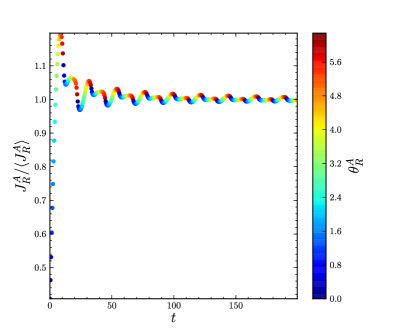
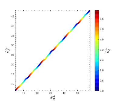
Figure 13.— Action–angle calculations using an orbit-integration-based method. The left panel shows the cumulative mean of the radial actions calculated in an auxiliary isochrone potential calculated along the orbit of the progenitor used in the main body of this paper. The color-coding corresponds to the radial angle (calculated in the isochrone potential) along the orbit. The time is in units of $35.56\,\mathrm{Myr}$ and the radial action is normalized by its value at $t=200$. The right panel shows the radial and vertical angles calculated in the auxiliary isochrone potential, with color-coding corresponding to the azimuthal angle. The wiggles in the angles are due to the isochrone potential not being the correct potential, but these wiggles are fit and removed to calculate the true angles.

The Fox method consists of averaging equation (A2) over the three-dimensional torus $\boldsymbol{\theta}^{a}$ covered by the orbit, such that the mapping defined by the $S_{\mathbf{n}}$ is onto orbital tori of the target Hamiltonian, the oscillating cosine behavior cancels, and the target actions are obtained as the auxiliary-angles-averaged auxiliary actions. Performing these three-dimensional integrals is difficult, because it is necessary to approximate the three-dimensional volume $\mathrm{d}\boldsymbol{\theta}^{A}$ from a one-dimensional set of points along the integrated orbit. Here I show that the three-dimensional integrals over $\boldsymbol{\theta}^{A}$ can be simplified for non-resonant orbits to one-dimensional integrals over one of the auxiliary angles along the path of the orbit. This significantly simplifies the calculations, especially of $J_{\phi}$ and $J_{Z}$ (see below). That is, we integrate over equation (A2) as

$$\int\mathrm{d}\theta_{i}^{A}J_{i}^{A}=\int\mathrm{d}\theta_{i}^{A}J_{i}+2\sum_{\mathbf{n}>0}\mathbf{n}\,S_{\mathbf{n}}(J_{i})\int\mathrm{d}\theta_{i}^{A}\cos(\mathbf{n}\cdot\boldsymbol{\theta}^{A})\,,$$ (A4)

where the integral is over auxiliary angles calculated on the path of the orbit in the target potential. The factor $\mathbf{n}\,S_{\mathbf{n}}(J_{i})$ comes out of the integral as the target actions are conserved along the orbit. In this Equation, we integrate over the angle coordinate $\theta_{i}^{A}$ associated with the action $J_{i}$ that we want to compute (that is, $\theta_{R}$ for $J_{R}$ and so on). This is because of the factor $\mathbf{n}$: the condition $\mathbf{n}>0$ means that when calculating $J_{R}$ there are terms with $\mathbf{n}=(n_{R},0,0)$, which would not cancel according to the argument below when integrating over $\theta_{Z}$. For non-resonant orbits and after a long-enough orbit integration, the angles can be considered to be independent (that is, the orbit “fills its torus”), such that we can write (for example, for $\theta_{R}$)

$$\begin{split}\int\mathrm{d}\theta_{R}^{A}\cos(\mathbf{n}\cdot\boldsymbol{\theta}^{A})&=\mathrm{Re}\left[\int\mathrm{d}\theta_{R}^{A}\,\exp(-i\mathbf{n}\cdot\boldsymbol{\theta}^{A})\right]\,,\\ &\approx\mathrm{Re}\left[\exp(-i\,n_{\phi}\,\theta^{A}_{\phi}-i\,n_{Z}\,\theta^{A}_{Z})\int\mathrm{d}\theta_{R}^{A}\,\exp(-i\,n_{R}\,\theta^{A}_{R})\right]\,.\end{split}$$ (A5)

As long as the auxiliary angle $\theta^{A}_{R}$ goes through the full range $0$ to $2\pi$ along the orbit, the oscillatory behavior integrates to zero and equation (A4) simplifies to

$$J_{i}=\frac{\int\mathrm{d}\theta_{i}^{A}J_{i}^{A}}{\int\mathrm{d}\theta_{i}^{A}}\,,$$ (A6)

that is, the target action is obtained by averaging the auxiliary action over the auxiliary angle.

The left panel of Figure 13 shows a running average of the radial action calculated using equation (A6) along the orbit of the progenitor in the simulation used in the main body of this paper. The time in this figure is in units of $35.56\,\mathrm{Myr}$, so the orbit is integrated for a total of $7.11\,\mathrm{Gyr}$. The auxiliary isochrone potential has a scale parameter of $6.4\,\mathrm{kpc}$. After a few radial periods, the radial action quickly converges with a remaining oscillatory behavior that is primarily a function of the radial angle, but that becomes smaller over time. With longer integrations and shorter time-steps, the radial action can converge to any desired tolerance. The duration of the orbit integration shown in this figure is what is typically used in this paper and gives a precision of $\approx 2\,\%$ in the actions.

Given the orbit integration already performed for calculating the actions, we can use equation (A3) to calculate the frequencies and angles corresponding to the point $(\mathbf{x},\mathbf{v})$ (this procedure is similar to that used in McMillan & Binney 2008). We first re-write equation (A3) in terms of the angle at time zero and the frequencies

$$\boldsymbol{\theta}=\boldsymbol{\theta}(t=0)+\mathbf{\Omega}(\mathbf{J})\,t=\boldsymbol{\theta}^{A}+2\sum_{\mathbf{n}>0}\frac{\partial S_{\mathbf{n}}(\mathbf{J})}{\partial\mathbf{J}}\,\sin(\mathbf{n}\cdot\boldsymbol{\theta}^{A})\,.$$ (A7)

This is a linear system of equations for each point along the orbit with unknowns $\boldsymbol{\theta}(t=0)$, $\mathbf{\Omega}(\mathbf{J})$, and the functions $\frac{\partial S_{\mathbf{n}}(\mathbf{J})}{\partial\mathbf{J}}$. For a finely integrated orbit, this system is highly over-constrained (at least when the number of expansion terms is small) and its solution can be found by simple linear algebra for any desired number of expansion terms $\sin(\mathbf{n}\cdot\boldsymbol{\theta}^{A})$. For extra stability, I integrate the orbit both forward and backward in time, such that the desired angle $\boldsymbol{\theta}(t=0)$ is at the center of the dependent variable $t$.

The right panel of Figure 13 shows the auxiliary radial angle versus the auxiliary vertical angle along the orbit for the progenitor used in the main body of this paper. The periodic behavior in the angles is removed before the linear fit described in the previous paragraph, which is shown in this figure. It is clear that the contribution of the oscillatory terms $\sin(\mathbf{n}\cdot\boldsymbol{\theta}^{A})$ is small, such that a small number of expansion terms is sufficient (I limit the terms in this axisymmetric case to $n_{R}<4$ and $n_{Z}<4$).

The method described here is completely general and the only obstacle to using it is that a sufficiently close isochrone potential has to be supplied. Sufficiently close means specifically that the auxiliary angles have to go through the full range of $0$ to $2\pi$ along the orbit in the target potential. Whether they do or not is easy to check and I have found that with limited trial and error a good enough isochrone potential can be determined quickly for Milky-Way-like axisymmetric potentials in regions where the flattening is mild (i.e., in the halo). Whether this method works near the plane of the disk where the potential is strongly flattened remains to be checked, although the fact that disk orbits are close to circular makes the details of the auxiliary potential unimportant. Similarly, the method should be tested in more detail for triaxial potentials as well. For analyzing stream data, the necessity of this trial-and-error determination of the auxiliary potential does not pose a practical problem, as all of the stream stars are on very similar orbits. Therefore, the same auxiliary potential can be used for all action–angle calculations for a given potential and for different potentials as well, as long as they are not too different. More widespread use of this technique may require automated methods for determining a good auxiliary potential. In the unlikely circumstance that no good auxiliary isochrone potential can be found, the method discussed here can also be used with other auxiliary potentials for which the actions and angles can be calculated, such as other spherical potentials or the family of Stäckel potentials. This will, however, add a non-negligible amount of computation for the necessary numerical integrations.

After this paper appeared, a similar technique for calculating actions, frequencies, and angles was presented by Sanders & Binney (2014). Their technique fits for the coefficients of $\cos(\mathbf{n}\cdot\boldsymbol{\theta}^{A})$ in equation (A2) to obtain the actions (similar to how we obtain the frequencies and angles here) rather than just averaging the auxiliary actions as in equation (A6). They also include a discussion of how to handle box orbits and a more detailed procedure for finding a good auxiliary potential. They explicitly and in detail demonstrate that this new procedure for calculating action–angle coordinates works well for triaxial potentials.

The action–angle method described in this Appendix is implemented in the galpy Galactic dynamics code.

References

- Binney & Tremaine (2008) Binney, J. & Tremaine, S. 2008, Galactic Dynamics: Second Edition
- Binney (2008) Binney, J. 2008, MNRAS, 386, L47
- Binney (2012) Binney, J. 2012, MNRAS, 426, 1324
- Bovy et al. (2011) Bovy, J., Hogg, D. W., & Roweis, S. T. 2011, Ann. Appl. Stat. 5, 1657, arXiv:0905.2979v1
- Carlberg (2012) Carlberg, R. G. 2012, ApJ, 748, 20
- Dehnen (2000) Dehnen, W. 2000, ApJ, 536, L39
- Dehnen (2002) Dehnen, W. 2002, J. Comput. Phys., 179, 27
- Eyre & Binney (2011) Eyre, A. & Binney, J. 2011, MNRAS, 413, 1852
- Fox (2012) Fox, M. 2012, M. Phys. thesis, Univ. Oxford, arXiv:1407.1688
- Gilks & Wild (1992) Gilks, W. R. & Wild, P. 1992, Applied Statistics, 41, 337
- Helmi & White (1999) Helmi, A. & White, S. D. M. 1999, MNRAS, 307, 495
- Johnston (1998) Johnston, K. V. 1998, ApJ, 495, 297
- Johnston et al. (1999) Johnston, K. V., Zhao, H., Spergel, D. N., & Hernquist, L. 1999, ApJ, 512, L109
- King (1966) King, I. R. 1966, AJ, 71, 64
- Koposov et al. (2010) Koposov, S. E., Rix, H.-W., & Hogg, D. W. 2010, ApJ, 712, 260
- Küpper et al. (2010) Küpper, A. H. W., Kroupa, P., Baumgardt, H., & Heggie, D. C. 2010, MNRAS, 401, 105
- Law et al. (2005) Law, D. R., Johnston, K. V., & Majewski, S. R. 2005, ApJ, 619, 807
- McGill & Binney (1990) McGill, C. & Binney, J. 1990, MNRAS, 244, 634
- McMillan & Binney (2008) McMillan, P. J. & Binney, J. J. 2008, MNRAS, 390, 429
- Ngan & Carlberg (2014) Ngan, W. H. W. & Carlberg, R. G. 2014, ApJ, 788, 181
- Peñarrubia et al. (2012) Peñarrubia, J., Koposov, S. E., & Walker, M. G. 2012, ApJ, 760, 2
- Perryman et al. (2001) Perryman, M. A. C., et al. 2001, A&A, 369, 339
- Price-Whelan & Johnston (2013) Price-Whelan, A. M. & Johnston, K. V. 2013, ApJ, 778, L12
- Sanders (2012) Sanders, J. 2012, MNRAS, 426, 128
- Sanders & Binney (2013a) Sanders, J. L. & Binney, J. 2013a, MNRAS, 433, 1813
- Sanders & Binney (2013b) Sanders, J. L. & Binney, J. 2013b, MNRAS, 433, 1826
- Sanders (2014) Sanders, J. L. 2014, MNRAS, 443, 423
- Sanders & Binney (2014) Sanders, J. L. & Binney, J. 2014, MNRAS, 441, 3284
- Sesar et al. (2013) Sesar, B., Grillmair, C. J., Cohen, J. G., et al. 2013, ApJ, 776, 26
- Shoemake (1985) Shoemake, K. 1985, ACM SIGGRAPH Computer Graphics 3, 45
- Teuben (1995) Teuben, P. J. 1995, in Astronomical Data Analysis Software and Systems IV, ed. R. Shaw, H. E. Payne and J. J. E. Hayes., PASP Conf Series 77, 398
- Tremaine (1999) Tremaine, S. 1999, MNRAS, 307, 877
- Varghese et al. (2011) Varghese, A., Ibata, R., & Lewis, G. F. 2011, MNRAS, 417, 198
- Yoon et al. (2011) Yoon, J. H., Johnston, K. V., & Hogg, D. W. 2011, ApJ, 731, 58