Binary Classifier Calibration: A Bayesian Non-Parametric Approach

Abstract

A set of probabilistic predictions is well calibrated if the events that are predicted to occur with probability $p$ do in fact occur about $p$ fraction of the time. Well calibrated predictions are particularly important when machine learning models are used in decision analysis. This paper presents two new non-parametric methods for calibrating outputs of binary classification models: a method based on the Bayes optimal selection and a method based on the Bayesian model averaging. The advantage of these methods is that they are independent of the algorithm used to learn a predictive model, and they can be applied in a post-processing step, after the model is learned. This makes them applicable to a wide variety of machine learning models and methods. These calibration methods, as well as other methods, are tested on a variety of datasets in terms of both discrimination and calibration performance. The results show the methods either outperform or are comparable in performance to the state-of-the-art calibration methods.

1 Introduction

This paper focuses on the development of probabilistic calibration methods for probabilistic prediction tasks. Traditionally, machine-learning research has focused on the development of methods and models for improving discrimination, rather than on methods for improving calibration. However, both are very important. Well-calibrated predictions are particularly important in decision making and decision analysis niculescu2005predicting ; zadrozny2001obtaining ; zadrozny2002transforming . Miscalibrated models, which overestimate or underestimate the probability of outcomes, may lead to making suboptimal decisions.

Since calibration is often not a priority, many prediction models learned by machine learning methods may be miscalibrated. The objective of this work is to develop general but effective methods that can address the miscalibration problem. Our aim is to have methods that can be used independent of the prediction model and that can be applied in the post-processing step after the model is learned from the data. This approach frees the designer of the machine learning model from the need to add additional calibration measures and terms into the objective function used to learn the model. Moreover, all modeling methods make assumptions, and some of those assumptions may not hold in a given application, which could lead to miscalibration. In addition, limited training data can negatively affect a model’s calibration performance.

Existing calibration methods can be divided into parametric and non-parametric methods. An example of a parametric method is Platt s method that applies a sigmoidal transformation that maps the output of a model (e.g., a posterior probability) platt1999probabilistic to a new probability that is intended to be better calibrated. The parameters of the sigmoidal transformation function are learned using the maximum likelihood estimation framework. A limitation of the sigmoidal function is that it is symmetric and does not work well for highly biased distributions jiang2012calibrating . The most common non-parametric methods are based either on binning zadrozny2001obtaining or isotonic regression ayer1955empirical . Briefly, the binning approach divides the observed outcome predictions into k bins; each bin is associated with a new probability value that is derived from empirical estimates. The isotonic regression algorithm is a special adaptive binning approach that assures the isotonicity (monotonicity) of the probability estimates.

In this paper we introduce two new Bayesian non-parametric calibration methods. The first one, the Selection over Bayesian Binnings $(SBB)$, uses dynamic programming to efficiently search over all possible binnings of the posterior probabilities within a training set in order to select the Bayes optimal binning according to a scoring measure. The second method, Averaging over Bayesian Binnings $(ABB)$, generalizes $SBB$ by performing model averaging over all possible binnings. The advantage of these Bayesian methods over existing calibration methods is that they have more stable, well-performing behavior under a variety of conditions.

Our probabilistic calibration methods can be applied in two prediction settings. First, they can be used to convert the outputs of discriminative classification models, which have no apparent probabilistic interpretation, into posterior class probabilities. An example is an SVM that learns a discriminative model, which does not have a direct probabilistic interpretation. Second, the calibration methods can be applied to improve the calibration of predictions of a probabilistic model that is miscalibrated. For example, a Naïve Bayes (NB) model is a probabilistic model, but its class posteriors are often miscalibrated due to unrealistic independence assumptions niculescu2005predicting . The methods we describe are shown empirically to improve the calibration of NB models without reducing its discrimination. The methods can also work well on calibrating models that are less egregiously miscalibrated than are NB models.

The remainder of this paper is organized as follows. Section 2 describes the methods that we applied to perform post-processing calibration. Section 3 describes the experimental setup that we used in evaluating the calibration methods. The results of the experiments are presented in Section 4. Section 5 discusses the results and describes the advantages and disadvantages of proposed methods in comparison to other calibration methods. Finally, Section 6 states conclusions, and describes several areas for future work.

2 Methods

In this section we present two new Bayesian non-parametric methods for binary classifier calibration that generalize the histogram-binning calibration method zadrozny2001obtaining by considering all possible binnings of the training data. The first proposed method, which is a hard binning classifier calibration method, is called Selection over Bayesian Binnings $(SBB)$. We also introduce a new soft binning method that generalizes $SBB$ by model averaging over all possible binnings; it is called Averaging over Bayesian Binnings $(ABB)$. There are two main challenges here. One is how to score a binning. We use a Bayesian score. The other is how to efficiently search over such a large space of binnings. We use dynamic programming to address this issue.

2.1 Bayesian Calibration Score

Let $p_{in}^{i}$ and $Z_{i}$ define respectively an uncalibrated classifier prediction and the true class of the $i$’th instance . Also, let $D$ define the set of all training instances $(p_{in}^{i},Z_{i})$. In addition, let $S$ be the sorted set of all uncalibrated classifier predictions $\{p_{in}^{1},p_{in}^{2},\ldots,p_{in}^{N}\}$ and $S_{l,u}$ be a list of the first elements of $S$, starting at $l$’th index and ending at $u$’th index, and let $Pa$ denote a binning of $S$. A binning model $M$ induced by the training set is defined as:

$$M\equiv\{B,S,Pa,\Theta\},$$ (1)

where, $B$ is the number of bins over the set $S$ and $\Theta$ is the set of all the calibration model parameters $\Theta=\{\theta_{1},\ldots,\theta_{B}\}$, which are defined as follows. For a bin $b$, which is determined by $S_{l_{b},u_{b}}$, the distribution of the class variable $P(Z=1|B=b)$ is modeled as a binomial distribution with parameter $\theta_{b}$. Thus, $\Theta$ specifies all the binomial distributions for all the existing bins in $Pa$. We note that our binning model is motivated by the model introduced in jonathan12application for variable discretization, which is here customized to perform classifier calibration. We score a binning model $M$ as follows:

$$Score(M)=P(M)\cdot P(D|M)$$ (2)

The marginal likelihood $P(D|M)$ in Equation 2 is derived using the marginalization of the joint probability of $P(D,\Theta)$ over all parameter space according to the following equation:

$$P(D|M)=\int_{\Theta}P(D|M,\Theta)P(\Theta|M)d_{\Theta}$$ (3)

Equation 3 has a closed form solution under the following assumptions: (1) All samples are i.i.d and the class distribution $P(Z|B=b)$ ,which is class distribution for instances locatd in bin number $b$, is modeled using a binomial distribution with parameter $\theta_{b}$, (2) the distribution of class variables over two different bins are independent of each other, and (3) the prior distribution over binning model parameters $\theta$s are modeled using a $Beta$ distribution. We also assume that the parameters of the $Beta$ distribution $\alpha$ and $\beta$ are both equal to one, which means corresponds to a uniform distribution over each $\theta_{b}$. The closed form solution to the marginal likelihood given the above assumptions is as follows heckerman1995learning :

$$P(D|M)=\prod_{b=1}^{B}\frac{n_{b0}!\hskip 1.99997ptn_{b1}!}{(n_{b}+1)!},$$ (4)

where $n_{b}$ is the total number of training instances located in bin $b$. Also, $n_{b0}$ and $n_{b1}$ are respectively the number of class zero and class one instances among all $n_{b}$ training instances in bin $b$.

The term $P(M)$ in Equation 2 specifies the prior probability of a binning of calibration model $M$. It can be interpreted as a structure prior, which we define as follows. Let $Prior(k)$ be the prior probability of there being a partitioning boundary between $p_{in}^{k}$ and $p_{in}^{k+1}$ in the binning given by model $M$, and model it using a $Poisson$ distribution with parameter $\lambda$.

Consider the prior probability for the presence of bin $b$, which contains the sequence of training instances $S_{l_{b},u_{b}}$ according to model $M$. Assuming independence of the appearance of partitioning boundaries, we can calculate the prior of the boundaries defining bin $b$ by using the $Prior$ function as follows:

$$Prior(u_{b})\left(\prod_{k=l_{b}}^{u_{b}-1}(1-Prior(k))\right)$$ (5)

where the product is over all training instances from $S_{l_{b}}$ to $S_{u_{b}-1}$ , inclusive.

Combining Equations 5 and 4 into Equation 2, we obtain the following Bayesian score for calibration model $M$:

$${Score(M)=\prod_{b=1}^{B}\left[Prior(u_{b})\left(\prod_{k=l_{b}}^{u_{b}-1}(1-Prior(k))\right)\frac{n_{b0}!\hskip 1.99997ptn_{b1}!}{(n_{b}+1)!}\right]}$$ (6)

2.2 The $SBB$ and $ABB$ models

We can use the above Bayesian score to perform model selection or model averaging. Selection involves choosing the best partitioning model $M_{opt}$ and calibrating a prediction $x$ as $P(x)=P(x|M_{opt})$. As mentioned, we call this approach Selection over Bayesian Binnings $(SBB)$. Model averaging involves calibrating predictions over all possible binnings. We call this approach Averaging over Bayesian Binnings $(ABB)$ model. A calibrated prediction in $ABB$ is derived as follows:

$$\begin{split}P(x)&=\sum_{i=1}^{2^{N-1}}P(M_{i}|D)P(x|M_{i})\\ &\propto\sum_{i=1}^{2^{N-1}}Score(M_{i})P(x|M_{i}),\end{split}$$ (7)

where $N$ is the total number of predictions in $D$ (i.e., training instances).

Both $(SBB)$ and $(ABB)$ consider all possible binnings of the $N$ predictions in $D$, which is exponential in $N$. Thus, in general, a brute-force approach is not computationally tractable. Therefore, we apply dynamic programming, as described in the next two sections.

2.3 Dynamic Programming Search of $SBB$

This section summarizes the dynamic programming method used in $SBB$. It is based on the dynamic-programming-based discretization method described in jonathan12application . Recall that $S$ is the sorted set of all uncalibrated classifier’s outputs $\{p_{in}^{1},p_{in}^{2},\ldots,p_{in}^{N}\}$ in the training data set. Let $S_{1,u}$ define the prefix of set $S$ including the set of the first $u$ uncalibrated estimates $\{p_{in}^{1},p_{in}^{2},\ldots,p_{in}^{u}\}$. Consider finding the optimal binning models $M_{1,u}$ corresponding to the subsequence $S_{1,u}$ for $u\in{1,2,\ldots,N}$ of the set $S$. Assume we have already found the highest score binning of these models $M_{1,1},M_{1,2},\ldots,M_{1,u-1}$, corresponding to each of the subsequences $S_{1,1},S_{1,2},\ldots,S_{1,u-1}$. Let $V^{f}_{1},V^{f}_{2},\ldots,V^{f}_{u-1}$ denote the respective scores of the optimal binnings of these models. Let $Score_{i,u}$ be the score of subsequence $\{p_{in}^{i},p_{in}^{2},\ldots,p_{in}^{u}\}$ when it is considered as a single bin in the calibration model $M_{1,u}$. For all $l$ from $u$ to $1$, $SBB$ computes $V^{f}_{l-1}\times Score_{l,u}$, which is the score for the highest scoring binning $M_{1,u}$ of set $S_{1,u}$ for which subsquence $S_{l,u}$ is considered as a single bin. Since this binning score is derived from two other scores , we call it a composite score of the binning model $M_{1,u}$. The fact that this composite score is a product of two scores follows from the decomposition of Bayesian scoring measure we are using, as given by Equation 6. In particular, both the prior and marginal likelihood terms on the score are decomposable.

In finding the best binning model $M_{1,u}$, $SBB$ chooses the maximum composite score over all $l$, which corresponds to the optimal binning for the training data subset $S_{1,u}$; this score is stored in $V^{f}_{u}$. By repeating this process from $1$ to $N$, $SBB$ derives the optimal binning of set $S_{1,N}$, which is the best binning over all possible binnings. As shown in jonathan12application , the computational time complexity of the above dynamic programming procedure is $O(N^{2})$.

2.4 Dynamic Programming Search of $ABB$

The dynamic programming approach used in $ABB$ is based on the above dynamic programming approach in $SBB$. It focuses on calibrating a particular instance $P(x)$. Thus, it is an instance-specific method. The $ABB$ algorithm uses the $decomposability$ property of the Bayesian binning score in Equation 6. Assume we have already found in one forward run (from lowest to highest prediction) of the $SBB$ method the highest score binning of the models $M_{1,1},M_{1,2},\ldots,M_{1,N}$, which correspond to each of the subsequences $S_{1,1},S_{1,2},\ldots,S_{1,N}$, respectively; let the values $V^{f}_{1},V^{f}_{2},\ldots,V^{f}_{N}$ denote the respective scores of the optimal binning for these models, which we cache. We perform an analogous dynamic programming procedure in $SBB$ in a backward manner (from highest to lowest prediction) and compute the highest score binning of these models $M_{N,N},M_{N-1,N},\ldots,M_{1,N}$, which correspond to each of the subsequences $S_{N,N},S_{N-1,N},\ldots,S_{1,N}$, respectively; let the values $V^{b}_{N},V^{b}_{N-1},\ldots,V^{b}_{1}$ denote the respective scores of the optimal binning for these models, which also cache. Using the decomposability property of the binning score given by 6, we can write the Bayesian model averaging estimate given by Equation 7 as follows:

$$P(x)\propto\sum_{1\leq l\leq u\leq N}\left(V^{f}_{l-1}\times Score_{l,u}\times V^{b}_{u+1}\times\hat{p}_{l,u}(x)\right)$$ (8)

where $\hat{p}_{l,u}(x)$ is obtained using the frequency of the training instances in the bin containing the predictions $S_{l,u}$. Remarkably, the dynamic programming implementation of $ABB$ is also $O(N^{2})$. However, since it is instance specific, this time complexity holds for each prediction that is to be calibrated (e.g., each prediction in a test set). To address this problem, we can partition the interval [0, 1] into $R$ equally spaced bins and stored the ABB output for each of those bins. The training time is therefore $O(RN^{2})$. During testing, a given $p_{in}$ is mapped to one of the $R$ bins and the stored calibrated probability is retrieved, which can all be done in $O(1)$ time.

3 Experimental Setup

This section describes the set of experiments that we performed to evaluate the calibration methods described above. To evaluate the calibration performance of each method, we ran experiments using both simulated data and real data. In our experiments on simulated data, we used logistic regression (LR) as the base classifier, whose predictions are to be calibrated. The choice of logistic regression was made to let us compare our results with the state-of-the-art method $ACP$, which as published is tailored for LR. For the simulated data, we used one dataset in which the outcomes were linearly separable and two other datasets in which they were not. Also, in the simulation data we used $600$ randomly generated instances for training LR model, $600$ random instances for learning calibration-models, and $600$ random instances for testing the models The scatter plots of the two linearly non-separable simulated datasets are shown in Figures [2, 2 ].

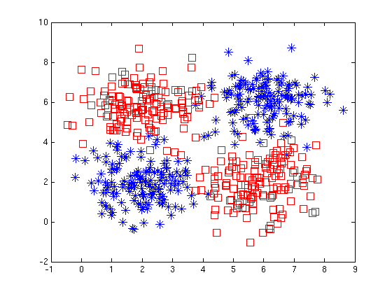
Figure 1: XOR Configuration

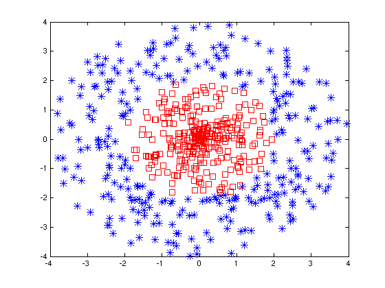
Figure 2: Circular Configuration

We also performed experiments on three different sets of real binary classification data. The first set is the UCI Adult dataset. The prediction task is a binary classification problem to predict whether a person makes over $50K a year using his or her demographic information. From the original Adult dataset, which includes $48842$ total instances with $14$ real and categorical features, after removing the instances with missing values, we used $2000$ instances for training classifiers, $600$ for calibration-model learning, and $600$ instances for testing.

We also used the UCI SPECT dataset, which is a small biomedical binary classification dataset. SPECT allows us to examine how well each calibration method performs when the calibration dataset is small in a real application. The dataset involves the diagnosis of cardiac Single Proton Emission Computed Tomography (SPECT) images. Each of the patients is classified into two categories: normal or abnormal. This dataset consists of $80$ training instances, with an equal number of positive and negative instances, and $187$ test instances with only $15$ positive instances. The SPECT dataset includes $22$ binary features. Due to the small number of instances, we used the original training data as both our training and calibration datasets, and we used the original test data as our test dataset.

For the experiments on the Adult and SPECT datasets, we used three different classifiers: LR, naïve Bayes, and SVM with polynomial kernels. The choice of the LR model allows us to include the ACP method in the comparison, because as mentioned it is tailored to LR. Naïve Bayes is a well-known, simple, and practical classifier that often achieves good discrimination performance, although it is usually not well calibrated. We included SVM because it is a relatively modern classifier that is being frequently applied.

The other real dataset that we used for evaluation contains clinical findings (e.g., symptoms, signs, laboratory results) and outcomes for patients with community acquired pneumonia (CAP) fine1997prediction . The classification task we examined involves using patient findings to predict dire patient outcomes, such as mortality or serious medical complications. The CAP dataset includes a total of $2287$ patient cases (instances) that we divided into $1087$ instances for training of classifiers, $600$ instances for learning calibration models, and $600$ instances for testing the calibration models. The data includes $172$ discrete and $43$ continuous features. For our experiments on the naïve Bayes model, we just used the discrete features of data, and for the experiments on SVM we used all $215$ discrete and continuous features. Also, for applying LR model to this dataset, we first used PCA feature transformation because of the high dimensionality of data and the existing correlations among some features, which produced unstable results due to singularity issues.

4 Experimental Results

This section presents experimental results of the calibration methods when applied to the datasets described in the previous section. We show the performance of the methods in terms of both calibration and discrimination, since in general both are important. Due to a lack of space, we do not include here the results for the linearly separable data; however, we note that the results for each of the calibration methods and the base classifier was uniformly excellent across the different evaluation measures that are described below.

For the evaluation of the calibration methods, we used $5$ different measures. The first two measures are Accuracy (Acc) and the Area Under the ROC Curve (AUC), which measure discrimination. The three other measures are the Root Mean Square Error (RMSE), Expected Calibration Error (ECE), and Maximum Calibration Error (MCE). These measures evaluate calibration performance. The $ECE$ and $MCE$ are simple statistics that measure calibration relative to the ideal reliability diagram degroot1983comparison ; niculescu2005predicting . In computing these measures, the predictions are partitioned to ten bins $\{[0,.1),[.1,.2),\ldots,[.9,1]\}$. The predicted value of each test instance falls into one of the bins. The $ECE$ calculates Expected Calibration Error over the bins, and $MCE$ calculates the Maximum Calibration Error among the bins, using empirical estimates as follows:

$$ECE = \sum_{i=1}^{10}P(i)\cdot\left|o_{i}-e_{i}\right|$$

$$MCE = \max\left(\left|o_{i}-e_{i}\right|\right)$$

where $o_{i}$ is the true fraction of positive instances in bin $i$, $e_{i}$ is the mean of the post-calibrated probabilities for the instances in bin $i$, and $P(i)$ is the empirical probability (fraction) of all instances that fall into bin $i$. The lower the values of $ECE$ and $MCE$, the better is the calibration of a model.

The Tables $[\ref{tab:SimulatedData1},\ref{tab:SimulatedData2},\ldots,\ref{tab:Pnuemonia_SVM}]$ show the comparisons of different methods with respect to evaluation measures on the simulated and real datasets. In these tables in each row we show in bold the two methods that achieved the best performance with respect to a specified measure.

As can be seen, there is no superior method that outperforms all the others in all data sets on all measures. However, SBB and ABB are superior to Platt and isotonic regression in all the simulation datasets. We discuss the reason why in Section 5. Also, SBB and ABB perform as well or better than isotonic regression and the Platt method on the real data sets.

In all of the experiments, both on simulated datasets and real data sets, both SBB and ABB generally retain or improve the discrimination performance of the base classifier, as measured by Acc and AUC. In addition, they often improve the calibration performance of the base classifier in terms of the $RMSE$, $ECE$ and $MCE$ measures.

5 Discussion

Having a well-calibrated classifier can be important in practical machine learning problems. There are different calibration methods in the literature and each one has its own pros and cons. The Platt method uses a sigmoid as a mapping function. The main advantage of Platt scaling method is its fast recall time. However, the shape of sigmoid function can be restrictive, and it often cannot produce well calibrated probabilities when the instances are distributed in feature space in a biased fashion (e.g. at the extremes, or all near separating hyper plane) jiang2012calibrating .

Histogram binning is a non-parametric method which makes no special assumptions about the shape of mapping function. However, it has several limitations, including the need to define the number of bins and the fact that the bins remain fixed over all predictions zadrozny2002transforming .

Isotonic regression-based calibration is another non-parametric calibration method, which requires that the mapping (from pre-calibrated predictions to post-calibrated ones) is chosen from the class of all isotonic (i.e., monotonicity increasing) functions niculescu2005predicting ; zadrozny2002transforming . Thus, it is less restrictive than the Platt calibration method. The pair adjacent violators (PAV) algorithm is one instance of an isotonic regression algorithm ayer1955empirical . The PAV algorithm can be considered as a binning algorithm in which the boundaries of the bins are chosen according to how well the classifier ranks the exampleszadrozny2002transforming . It has been shown that Isotonic regression performs very well in comparison to other calibration methods in real datasets niculescu2005predicting ; caruana2006empirical ; zadrozny2002transforming . Isotonic regression has some limitations, however. The most significant limitation of the isotonic regression is its isotonicity (monotonicity) assumption. As seen in Tables [2(a), 2(b)] in the simulation data, when the isotonicity assumption is violated through the choice of classifier and the nonlinearity of data, isotonic regression performs relatively poorly, in terms of improving the discrimination and calibration capability of a base classifier. The violation of this assumption can happen in real data secondary to the choice of learning models and algorithms.

A classifier calibration method called adaptive calibration of predictions (ACP) was recently introduced jiang2012calibrating . A given application of ACP is tied to a particular model $M$, such as a logistic regression model, that predicts a binary outcome $Z$. ACP requires a $95\%$ confidence interval (CI) around a particular prediction $p_{in}$ of $M$. ACP adjusts the CI and uses it to define a bin. It sets $p_{out}$ to be the fraction of positive outcomes $(Z=1)$ among all the predictions that fall within the bin. On both real and synthetic datasets, ACP achieved better calibration performance than a variety of other calibration methods, including simple histogram binning, Platt scaling, and isotonic regression jiang2012calibrating . The ACP post-calibration probabilities also achieved among the best levels of discrimination, according to the AUC. ACP has several limitations, however. First, it requires not only probabilistic predictions, but also a statistical confidence interval ($CI$) around each of those predictions, which makes it tailored to specific classifiers, such as logistic regression jiang2012calibrating . Second, based on a $CI$ around a given prediction $p_{in}$, it commits to a single binning of the data around that prediction; it does not consider alternative binnings that might yield a better calibrated $p_{out}$. Third, the bin it selects is symmetric around $p_{in}$ by construction, which may not optimize calibration. Finally, it does not use all of the training data, but rather only uses those predictions within the confidence interval around $p_{in}$. As one can see from the tables, ACP performed well when logistic regression is the base classifier, both in simulated and real datasets. SBB and ABB performed as well or better than ACP in both simulation and real data sets.

In general, the SBB and ABB algorithms appear promising, especially ABB, which overall outperformed SBB. Neither algorithm makes restrictive (and potentially unrealistic) assumptions, as does Platt scaling and isotonic regression. They also are not restricted in the type of classifier with which they can apply, unlike ACP.

The main disadvantage of SBB and ABB is their running time. If $N$ is the number of training instances, then SBB has a training time of $O(N^{2})$, due to its dynamic programming algorithm that searches over every possible binning, whereas the time complexity of ACP and histogram binning is $O(NlogN)$, and it is $O(N)$ for isotonic regression. Also, the cached version of ABB has a training time of $O(RN^{2})$, where $R$ reflects the number of bins being used. Nonetheless, it remains practical to use these algorithms to perform calibration on a desktop computer when using training datasets that contain thousands of instances. In addition, the testing time is only $O(b)$ for SBB where $b$ is the number of binnings found by the algorithm and $O(1)$ for the cached version of ABB. Table 1 shows the time complexity of different methods in learning for N training instances and recall for only one instance.

Table 1: Time complexity of calibration methods in learning and recall

	Platt	Hist	IsoReg	ACP	SBB	ABB
Time	$O(NT)/O(1)$	$O(NlogN)/O(b)$	$O(N)/O(b)$	$O(NlogN)/O(N)$	$O(N^{2})/O(b)$	$O(RN^{2})/O(1)$
Complexity
(Learning/Recall)
Note that N and b are the of training sets and the number of bins found by the method respectively. T is the number of iteration required for convergence in Platt method and R reflects the number of bins being used by cached ABB.

6 Conclusion

In this paper we introduced two new Bayesian, non-parametric methods for calibrating binary classifiers, which are called $SBB$ and $ABB$. Experimental results on simulated and real data support that these methods perform as well or better than the other calibration methods that we evaluated. While the new methods have a greater time complexity than the other calibration methods evaluated here, they nonetheless are efficient enough to be applied to training datasets with thousands of instances. Thus, we believe these new methods are promising for use in machine learning, particularly when calibrated probabilities are important, such as in decision analyses.

In future work, we plan to explore how the two new methods perform when using Bayesian model averaging over the hyper parameter $\lambda$. We also will extend them to perform multi-class calibration. Finally, we plan to investigate the use of calibration methods on posterior probabilities that are inferred from models that represent joint probability distributions, such as maximum-margin Markov-network models roller2004max ; zhu2008laplace ; zhu2009medlda .

Table 2: Experimental Results on Simulated and Real datasets

(a) Non-Linear XOR configuration results

	LR	ACP	IsoReg	Platt	Hist	SBB	ABB
AUC	0.497	0.950	0.704	0.497	0.931	0.914	0.941
Acc	0.510	0.887	0.690	0.510	0.855	0.887	0.888
RMSE	0.500	0.286	0.447	0.500	0.307	0.307	0.295
MCE	0.521	0.090	0.642	0.521	0.152	0.268	0.083
ECE	0.190	0.056	0.173	0.190	0.072	0.104	0.062

(b) Non-Linear Circular configuration results

	LR	ACP	IsoReg	Platt	Hist	SBB	ABB
AUC	0.489	0.852	0.635	0.489	0.827	0.816	0.838
Acc	0.500	0.780	0.655	0.500	0.795	0.790	0.773
RMSE	0.501	0.387	0.459	0.501	0.394	0.393	0.390
MCE	0.540	0.172	0.608	0.539	0.121	0.790	0.146
ECE	0.171	0.098	0.186	0.171	0.074	0.138	0.091

(c) Adult Naïve Bayes

	NB	IsoReg	Platt	Hist	SBB	ABB
AUC	0.879	0.876	0.879	0.877	0.849	0.879
Acc	0.803	0.822	0.840	0.818	0.838	0.835
RMSE	0.352	0.343	0.343	0.341	0.345	0.343
MCE	0.223	0.302	0.092	0.236	0.373	0.136
ECE	0.081	0.075	0.071	0.078	0.114	0.062

(d) Adult Linear SVM

	SVM	IsoReg	Platt	Hist	SBB	ABB
AUC	0.864	0.856	0.864	0.864	0.821	0.864
Acc	0.248	0.805	0.748	0.815	0.803	0.805
RMSE	0.587	0.360	0.434	0.355	0.362	0.357
MCE	0.644	0.194	0.506	0.144	0.396	0.110
ECE	0.205	0.085	0.150	0.077	0.108	0.061

(e) Adult Logistic Regression

	LR	ACP	IsoReg	Platt	Hist	SBB	ABB
AUC	0.730	0.727	0.732	0.730	0.743	0.699	0.731
Acc	0.755	0.783	0.753	0.755	0.753	0.762	0.762
RMSE	0.403	0.402	0.403	0.405	0.400	0.401	0.401
MCE	0.126	0.182	0.491	0.127	0.274	0.649	0.126
ECE	0.075	0.071	0.118	0.079	0.092	0.169	0.076

(f) SPECT Naïve Bayes

	NB	IsoReg	Platt	Hist	SBB	ABB
AUC	0.836	0.815	0.836	0.832	0.733	0.835
Acc	0.759	0.845	0.770	0.824	0.845	0.845
RMSE	0.435	0.366	0.378	0.379	0.368	0.374
MCE	0.719	0.608	0.563	0.712	0.347	0.557
ECE	0.150	0.141	0.148	0.145	0.149	0.157

(g) SPECT SVM Quadratic kernel

	SVM	IsoReg	Platt	Hist	SBB	ABB
AUC	0.816	0.786	0.816	0.766	0.746	0.810
Acc	0.257	0.834	0.684	0.845	0.813	0.813
RMSE	0.617	0.442	0.460	0.463	0.398	0.386
MCE	0.705	0.647	0.754	0.934	0.907	0.769
ECE	0.235	0.148	0.162	0.180	0.128	0.131

(h) SPECT Logistic Regression

	LR	ACP	IsoReg	Platt	Hist	SBB	ABB
AUC	0.744	0.742	0.733	0.744	0.738	0.733	0.741
Acc	0.658	0.561	0.626	0.668	0.620	0.620	0.626
RMSE	0.546	0.562	0.558	0.524	0.565	0.507	0.496
MCE	0.947	1.000	1.000	0.884	0.997	0.813	0.812
ECE	0.181	0.187	0.177	0.180	0.183	0.171	0.173

(i) CAP Naïve Bayes

	NB	IsoReg	Platt	Hist	SBB	ABB
AUC	0.848	0.845	0.848	0.831	0.775	0.838
Acc	0.730	0.865	0.847	0.853	0.832	0.865
RMSE	0.504	0.292	0.324	0.307	0.315	0.304
MCE	0.798	0.188	0.303	0.087	0.150	0.128
ECE	0.161	0.071	0.097	0.056	0.067	0.067

(j) CAP Linear SVM

	SVM	IsoReg	Platt	Hist	SBB	ABB
AUC	0.858	0.858	0.858	0.847	0.813	0.863
Acc	0.907	0.900	0.882	0.887	0.902	0.908
RMSE	0.329	0.277	0.294	0.287	0.285	0.274
MCE	0.273	0.114	0.206	0.110	0.240	0.121
ECE	0.132	0.058	0.093	0.057	0.083	0.050

(k) CAP Logistic Regression

	LR	ACP	IsoReg	Platt	Hist	SBB	ABB
AUC	0.920	0.910	0.917	0.920	0.901	0.856	0.921
Acc	0.925	0.932	0.935	0.928	0.897	0.935	0.932
RMSE	0.240	0.240	0.234	0.242	0.259	0.240	0.240
MCE	0.199	0.122	0.286	0.154	0.279	0.391	0.168
ECE	0.066	0.062	0.078	0.082	0.079	0.103	0.069

References

- [1] M. Ayer, HD Brunk, G.M. Ewing, WT Reid, and E. Silverman. An empirical distribution function for sampling with incomplete information. The annals of mathematical statistics, pages 641–647, 1955.
- [2] R. Caruana and A. Niculescu-Mizil. An empirical comparison of supervised learning algorithms. In Proceedings of the 23rd international conference on Machine learning, pages 161–168, 2006.
- [3] M.H. DeGroot and S.E. Fienberg. The comparison and evaluation of forecasters. The statistician, pages 12–22, 1983.
- [4] M.J. Fine, T.E. Auble, D.M. Yealy, B.H. Hanusa, L.A. Weissfeld, D.E. Singer, C.M. Coley, T.J. Marrie, and W.N. Kapoor. A prediction rule to identify low-risk patients with community-acquired pneumonia. New England Journal of Medicine, 336(4):243–250, 1997.
- [5] D. Heckerman, D. Geiger, and D.M. Chickering. Learning bayesian networks: The combination of knowledge and statistical data. Machine learning, 20(3):197–243, 1995.
- [6] X. Jiang, M. Osl, J. Kim, and L. Ohno-Machado. Calibrating predictive model estimates to support personalized medicine. Journal of the American Medical Informatics Association, 19(2):263–274, 2012.
- [7] J.L. Lustgarten, S. Visweswaran, V. Gopalakrishnan, and G.F. Cooper. Application of an efficient bayesian discretization method to biomedical data. BMC Bioinformatics, 12, 2011.
- [8] A. Niculescu-Mizil and R. Caruana. Predicting good probabilities with supervised learning. In Proceedings of the 22nd international conference on Machine learning, pages 625–632, 2005.
- [9] J. Platt et al. Probabilistic outputs for support vector machines and comparisons to regularized likelihood methods. Advances in large margin classifiers, 10(3):61–74, 1999.
- [10] B. Taskar, C. Guestri, and D. Koller. Max-margin markov networks. In Advances in Neural Information Processing Systems, volume 16, 2004.
- [11] B. Zadrozny and C. Elkan. Obtaining calibrated probability estimates from decision trees and naive bayesian classifiers. In Machine Learning-International Workshop then Conference, pages 609–616, 2001.
- [12] B. Zadrozny and C. Elkan. Transforming classifier scores into accurate multiclass probability estimates. In Proceedings of the eighth ACM SIGKDD international conference on Knowledge discovery and data mining, pages 694–699, 2002.
- [13] J. Zhu, A. Ahmed, and E.P. Xing. Medlda: maximum margin supervised topic models for regression and classification. In Proceedings of the 26th Annual International Conference on Machine Learning, pages 1257–1264, 2009.
- [14] J. Zhu, E.P. Xing, and B. Zhang. Laplace maximum margin markov networks. In Proceedings of the 25th international conference on Machine learning, pages 1256–1263, 2008.