Radial Covariance Functions Motivated by Spatial Random Field Models with Local Interactions

Abstract

Random fields based on energy functionals with local interactions possess flexible covariance functions, lead to computationally efficient algorithms for spatial data processing, and have important applications in Bayesian field theory. We derive explicit expressions for a family of radially symmetric, non-differentiable, Spartan covariance functions in $\mathbb{R}^{2}$ that involve the modified Bessel function of the second kind. In addition to the characteristic length and the amplitude coefficient, the Spartan covariance parameters include the rigidity coefficient ${\eta_{1}}$ which determines the shape of the covariance function. If ${\eta_{1}}\gg 1$ Spartan covariance functions exhibit multiscaling. We also derive a family of radially symmetric, infinitely differentiable Bessel-Lommel covariance functions valid in $\mathbb{R}^{d},d\geq 2$. We investigate the parametric dependence of the integral range for Spartan and Bessel-Lommel covariance functions using explicit relations and numerical simulations. Finally, we define a generalized spectrum of correlation scales $\lambda^{(\alpha)}_{c}$ in terms of the fractional Laplacian of the covariance function; for $0\leq\alpha\leq 1$ the $\lambda^{(\alpha)}_{c}$ extend from the smoothness microscale $(\alpha=1)$ to the integral range $(\alpha=0)$. The smoothness scale of mean-square continuous but non-differentiable random fields vanishes; such fields, however, can be discriminated by means of $\lambda^{(\alpha)}_{c}$ scales obtained for $\alpha<1$.

I Introduction

I-A Background

The theory of spatial random fields (SRFs) is a powerful mathematical framework for modelling spatial variability [1, 2, 3]. The SRF theory has a multidisciplinary scope of applications that include fluid mechanics [4], computational and probabilistic engineering mechanics [5], materials science [6, 7, 8], hydrological modeling [9, 10, 11], petroleum engineering [12, 13, 14], environmental monitoring [15, 16, 17], mining exploration and mineral reserves estimation [18, 19], environmental health [20], geophysical signal processing [21], image analysis [22, 23], machine learning [24]  statistical cosmology [25, 26], medical image registration [27], as well as in structural and functional mapping of the brain [28, 29, 30].

A second-order description of Gaussian or non-Gaussian, centered, scalar SRFs requires the introduction of a permissible covariance function, i.e., a non-negative definite, two-point function [31, 1]. Covariance functions are the key ingredient in Best Linear Unbiased Prediction (BLUP) methods for spatial interpolation and in geostatistical simulation [32, 33, 34, 35]. Covariance functions are also used as non-negative definite kernels in machine learning approaches based Gaussian processes [24, 36] as well as in radial basis function interpolation [37, 38] and surface reconstruction [39]. Valid covariance functions are employed in the simulation of non-Gaussian random fields via the Karhunen-Loève expansion [40, 41]. Most covariance functions used in the analysis of spatial data are mathematical constructions that satisfy Bochner’s theorem [31]. In principle, covariance functions can also be obtained from the solutions of stochastic partial differential equations [20, 42, 43] or from the solution of statistical field theories [44]. It is often impossible, however, to obtain closed-form covariance solutions for the entire distance range based on these approaches. The “standard” covariance models (e.g., the exponential, spherical, and Gaussian functions) involve two parameters: the variance and the correlation length. The variance determines the amplitude of the fluctuations, whereas all length scales characterizing SRF patterns are trivially proportional to the correlation length. Hence, two-parameter covariance models may fail to capture the variability of spatially distributed processes. Whereas some models with more than two parameters exist in the literature, e.g. the rational quadratic [45, 24], the Whittle-Matérn [46, 33], additional flexible covariance models are needed [45].

I-B Approach and Main Contributions

Our approach is based on SRFs governed by a Gibbs energy functional with local self-interactions [47]. The so-called Spartan spatial random fields (SSRFs) have a rational spectral density that involves a fourth degree polynomial in the denominator, c.f. equation (5) below. The energy functional is not meant to represent an actual energy of SRF configurations but to provide ad hoc geometric constraints that render SRF states with certain spatial patterns more likely than others. In one and three dimensions, explicit SSRF covariance expressions were derived at the limit of infinite ultraviolet (high-wavenumber) cutoff of the SSRF spectral density function [48].

The main contributions of this paper are threefold. First, we derive explicit expressions for stationary, non-differentiable, three-parameter, radial SSRF covariance functions ${\bf r}\in\mathbb{R}^{2}\mapsto C_{{\rm x}{\rm x}}({\bf r})\in\mathbb{R}$, and we show that these functions exhibit multiscaling in a specified region of the parameter space.

Secondly, we obtain stationary, infinitely differentiable, radial Bessel-Lommel covariance functions for ${\bf r}\in\mathbb{R}^{d},\,d\geq 2$ based on the reciprocal SSRF spectral density with finite spectral cutoff. These functions generalize the oscillatory ordinary Bessel covariance functions and provide covariance models for smooth spatial processes in $\mathbb{R}^{2}$ and $\mathbb{R}^{3}$. They can also be used in machine learning applications that involve higher-dimensional feature spaces [45, 24].

Thirdly, we define a generalized correlation spectrum that captures the integral ranges of fractional SRF derivatives. The spectrum can be used with both differentiable and non-differentiable stationary SRFs. In contrast with the smoothness microscale, which vanishes for mean square continuous but non-differentiable SRFs, the proposed spectrum discriminates between non-differentiable SRFs with different covariance functions.

I-C Structure

The remainder of this paper is structured as follows: Section II presents notation and mathematical background. Section III is a brief, non-mathematical overview of SSRFs. Section IV derives two-dimensional SSRF covariance functions at the limit of infinite ultraviolet cutoff of the spectral density. In Section V, Bessel-Lommel covariance functions in $d\geq 2$ are obtained. Section VI defines a generalized correlation spectrum and investigates its dependence for SSRF and Bessel-Lommel SRFs. Section VII investigates geometric features of Gaussian SRF realizations with SSRF and Bessel-Lommel covariance functions in connection with the results of Section VI. Section VIII summarizes the results and discusses potential applications. Most mathematical proofs are relegated to Appendices. Finally, Appendix E contains a table that summarizes the notation used.

II Definitions and Preliminaries

Given a complex number $z$, $\bar{z}$ denotes its complex conjugate; $\Re(z)$ and $\Im(z)$ denote respectively the real and imaginary parts of $z$, i.e., $z=\Re(z)+\jmath\,\Im(z)$. An operator $\mathbb{A}$ is self-adjoint if $\mathbb{A}=\mathbb{A}^{{\dagger}}$, where $\mathbb{A}^{{\dagger}}$ is the complex conjugate of $\mathbb{A}.$ The transpose of a vector or matrix ${\bf V}$ will be denoted by ${\bf V}^{T}$.

A scalar SRF $\{X({\bf s},\omega)\in\mathbb{R};\,{\bf s}\in\mathcal{D};\omega\in\Omega\}$ is a mapping from the probability space $(\Omega,A,P)$ into the space of real numbers so that for each fixed ${\bf s}$, $X({\bf s},\omega)$ is a measurable function of $\omega$ [1]. The spatial domain $\mathcal{D}$ includes all points ${\bf s}\in\mathbb{R}^{d}$. The reciprocal space involves the wavevectors ${\bf k}\in\mathbb{R}^{d}.$ In addition to $d$, we use as needed the dimension index $\nu=d/2-1$ to simplify notation. An SRF involves by definition a multitude of probable states or realizations indexed by $\omega$ [2, 15]. If $\Phi:\mathbb{R}\rightarrow\mathbb{R}$ is a Borel measurable function, then $\mathbb{E}\left[\Phi\left(X({\bf s},\omega)\right)\right]$ denotes the expectation of $\Phi\left(X({\bf s},\omega)\right)$ over the ensemble of states $\Omega$. A sample (realization) of the SRF will be denoted by $x({\bf s})\in\mathbb{R}.$

An SRF is second-order stationary or weakly stationary if (i) its expectation $\mathbb{E}[X({\bf s},\omega)]=m_{{\rm x}}$ is independent of the location and (ii) its autocovariance function depends only on the spatial lag vector ${\bf r}\in\mathbb{R}^{d}$ [2, pp. 308-438], i.e.,

$$C_{{\rm x}{\rm x}}({\bf r}) =\mathbb{E}[X({\bf s},\omega)X({\bf s}+{\bf r},\omega)]-m_{{\rm x}}^{2}.$$ (1)

In the following, we use the term “stationary” to refer to second-order stationarity. A stationary, scalar SRF is statistically isotropic (for short isotropic) if its covariance function is a radial function, i.e., if $C_{{\rm x}{\rm x}}({\bf r})=C_{{\rm x}{\rm x}}(\|{\bf r}\|)$, where $\|{\bf r}\|$ is the Euclidean norm of ${\bf r}$. In the following, we will use $r$ and $k$ to denote the Euclidean norms of the vectors ${\bf r}$ and ${\bf k}$ respectively .

II-A Spectral Representation

We review the spectral representation of covariance functions, since we will use it below to derive covariance functions in position space. For a stationary SRF let the Fourier transform of the covariance function from the space of lag vectors ${\bf r}\in\mathbb{R}^{d}$ to the reciprocal (Fourier) space of wavevectors ${\bf k}\in\mathbb{R}^{d}$ be defined by means of the following improper multiple integral:

$$\widetilde{C_{{\rm x}{\rm x}}}({\bf k};{\bm{\theta}})=\mathcal{F}[C_{{\rm x}{\rm x}}({\bf r};{\bm{\theta}})]=\int_{\mathbb{R}^{d}}d{\bf r}\;{\rm e}^{-\jmath\bf{k\cdot r}}C_{{\rm x}{\rm x}}({\bf r};{\bm{\theta}}),$$ (2)

where $d{\bf r}=\prod_{i=1}^{d}dr_{i}$. The inverse Fourier transform is then given by means of the improper multiple integral

$$C_{{\rm x}{\rm x}}({\bf r};{\bm{\theta}})=\mathcal{F}^{-1}[\widetilde{C_{{\rm x}{\rm x}}}({{\bf k}};{\bm{\theta}})]=\frac{1}{(2\,\pi)^{d}}\,\int_{\mathbb{R}^{d}}d{\bf k}\;{\rm e}^{\jmath\bf{k\cdot r}}\,\widetilde{C_{{\rm x}{\rm x}}}({\bf k};{\bm{\theta}}).$$ (3)

The integrals (2) and (3) are well defined if $C_{{\rm x}{\rm x}}({\bf r};{\bm{\theta}})$ and $\widetilde{C_{{\rm x}{\rm x}}}({\bf k};{\bm{\theta}})$ are absolutely integrable, respectively.

Theorem II.1.

Bochner-Khinchin’s permissibility theorem requires that

1. $\widetilde{C_{{\rm x}{\rm x}}}(k;{\bm{\theta}})>0,\,\forall{\bf k}$,

2. $\int_{\mathbb{R}^{d}}d{\bf k}\,\widetilde{C_{{\rm x}{\rm x}}}(k;{\bm{\theta}})<\infty$,

for the inverse Fourier transform (3) to represent a valid covariance function [31], [2, p.106].

For radial covariance functions the pair of transforms (2) and (3) is expressed as follows [2, p. 353]

$$\widetilde{C_{{\rm x}{\rm x}}}({k};{\bm{\theta}})=\frac{(2\pi)^{d/2}}{k^{\nu}}\int_{0}^{\infty}d{r}\,r^{d/2}{J_{\nu}(kr)}C_{{\rm x}{\rm x}}({r};{\bm{\theta}}),$$ (4a)

$$C_{{\rm x}{\rm x}}({r};{\bm{\theta}})=\frac{1}{(2\pi)^{d/2}r^{\nu}}\int_{0}^{\infty}d{k}\,k^{d/2}{J_{\nu}(kr)}\widetilde{C_{{\rm x}{\rm x}}}({k};{\bm{\theta}}),$$ (4b)

where $\nu=d/2-1$, $J_{\nu}(x),\,x\in\mathbb{R},$ is the Bessel function of the first kind of order $d/2-1,$ and $k$ is the Euclidean norm of the wavevector ${\bf k}$ [49].

III Review of Spartan Spatial Random Fields

Gibbs random fields have a joint probability density function defined in terms of an energy functional of the sample function $x({\bf s})$. Spartan Spatial Random Fields (SSRFs) are Gibbs random fields whose energy functional is defined in terms of local interactions between the values of $x({\bf s})$ at neighboring points. A particular type of SSRF is the Fluctuation-Gradient-Curvature FGC-SSRF  model whose energy functional involves the square gradient and the square Laplacian of $x({\bf s})$ [50, 48].

The SSRF model is determined by the parameter vector ${\bm{\theta}}=(\eta_{0},{\eta_{1}},\xi,{k_{c}})^{T},$ which includes the amplitude coefficient $\eta_{0}$, the characteristic length $\xi$, the rigidity coefficient ${\eta_{1}}$, and the spectral cutoff, ${k_{c}}$. The amplitude coefficient is analogous to temperature in statistical mechanics and controls the overall magnitude of the fluctuations. The rigidity coefficient controls the resistance of the field to changes of its gradient. The characteristic length controls, in conjunction with ${\eta_{1}}$, the relative strength of the square Laplacian versus the square gradient term. The spectral cutoff represents an implicit upper bound in reciprocal space, which should be finite for the SSRF states to be mean square differentiable (see Proposition 1 and its proof). We derive explicit covariance functions at the limit ${k_{c}}\rightarrow\infty$ where the SSRF states become non-differentiable in the mean square sense. These functions represent asymptotic limits of the covariance functions that correspond to the SSRF energy functional; they are nevertheless permissible, albeit non-differentiable, covariance functions.

The SSRF spectral density is given by the following function as shown in [47]

$$\widetilde{C_{{\rm x}{\rm x}}}({\bf k};{\bm{\theta}})=\frac{\eta_{0}\,\xi^{d}\,\mathbbm{1}_{{k_{c}}\geq k}(k)}{\Pi(k\xi)},$$ (5a)

$$\Pi(u)=1+{\eta_{1}}u^{2}+u^{4},$$ (5b)

where $\Pi(u)$, $u=k\,\xi$, is the characteristic polynomial of the SSRF spectral density, and $\mathbbm{1}_{A}(x)$ is the indicator function of the set $A$, i.e., $\mathbbm{1}_{A}(x)=1,\,x\in A$ and $\mathbbm{1}_{A}(x)=0,\,x\ni A.$

The non-negativity of $\widetilde{C_{{\rm x}{\rm x}}}({\bf k};{\bm{\theta}})$ —Condition (1) of Bochner’s theorem— is ensured $\forall{k_{c}}>0$, if ${\eta_{1}}>-2$ [47]. The integrability, Condition (2) of Bochner’s theorem, is satisfied for $\forall d\geq 1$, $\forall{k_{c}}\in\mathbb{R}_{+}$, or if ${k_{c}}\rightarrow\infty$ for $d<4$.

For radial SSRF covariance functions, the spectral representation is given by the following one-dimensional integral derived from (4b)

$$C_{{\rm x}{\rm x}}({r};{\bm{\theta}})=\frac{\eta_{0}\,\xi^{d}\,r^{1-d/2}}{(2\pi)^{d/2}}\int_{0}^{{k_{c}}}dk\frac{k^{d/2}J_{d/2-1}(kr)}{{1+\eta_{1}(k\xi)^{2}+(k\xi)^{4}}}.$$ (6)

The spectral integral (6) yields functions $C_{{\rm x}{\rm x}}({\bf r};{\bm{\theta}})$ in position space that change with $d$. In $\mathbb{R}^{1}$ and $\mathbb{R}^{3}$ the evaluation of the spectral integral (6) is facilitated by the fact that $J_{-1/2}(\cdot)$ and $J_{1/2}(\cdot)$ can be expressed in terms of trigonometric and algebraic functions respectively. The integral is then evaluated at the limit ${k_{c}}\rightarrow\infty$ using Cauchy’s Theorem of Residues [48]. Nonetheless, many “signals” of interest, including digital images and data from environmental sensor networks are strictly or approximately two-dimensional fields.

IV SSRF Covariance in Two Dimensions

Below we derive explicit expressions for SSRF covariance functions in $\mathbb{R}^{2}$ at the limit ${k_{c}}\rightarrow\infty$. The spectral integral (6) is expressed by the following Hankel transform of order zero:

$$C_{{\rm x}{\rm x}}({\bf r};{\bm{\theta}})=\frac{\eta_{0}\xi^{2}}{2\pi}\,\int\limits_{0}^{\infty}dk\,\frac{k\,J_{0}(kr)}{1+{\eta_{1}}(k\xi)^{2}+(k\xi)^{4}}.$$ (7)

Hankel transforms of integer order often do not admit explicit expressions. Nevertheless, the integral (7) is amenable to explicit evaluation by means of the Hankel-Nicholson integration formula [51, p. 488].

Proposition 1.

The SSRF covariance function in $\mathbb{R}^{2}$ defined by the integral (7) for ${\eta_{1}}>-2$ is given by the following equations

$$C_{{\rm x}{\rm x}}(h;{\bm{\theta}})=\frac{\eta_{0}\left[K_{0}(hz_{+})-K_{0}(hz_{-})\right]}{2\pi\sqrt{\eta_{1}^{2}-4}},\;{\eta_{1}}>2$$ (8a)

$$C_{{\rm x}{\rm x}}(h;{\bm{\theta}})=\left(\frac{\eta_{0}\,h}{4\pi}\right)\,K_{-1}(h),\;{\eta_{1}}=2.$$ (8b)

$$C_{{\rm x}{\rm x}}(h;{\bm{\theta}})=\frac{\eta_{0}\,\Im\left[K_{0}(hz_{+})\right]}{\pi\sqrt{4-\eta_{1}^{2}}},\;|{\eta_{1}}|<2,$$ (8c)

where $h=r/\xi$ is the dimensionless two-point lag distance, $K_{\nu}(\cdot)$ is the modified Bessel function of the second kind and order $\nu$, $\Im\left[\cdot\right]$ denotes the imaginary part, and

$$z_{\pm}^{2}={\left({\eta_{1}}\mp\Delta\right)}/{2}.$$ (9)

SSRFs with covariance functions given by (8) are continuous but non-differentiable in the mean square sense.

Proof:

The proof is given in the Appendix A. ∎

For ${\eta_{1}}=2$, Eq. (8b) recovers the known K-Bessel covariance function [34].

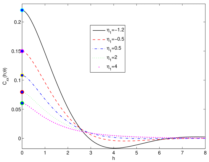
We illustrate the dependence of $C_{{\rm x}{\rm x}}(h;{\bm{\theta}})$ on $h$ for different ${\eta_{1}}$ in Fig. 1. For ${\eta_{1}}<0$, $C_{{\rm x}{\rm x}}(h;{\bm{\theta}})$ exhibits a negative peak and then returns to positive values; this damped oscillatory behavior is due to the peak of the spectral density for $-2<{\eta_{1}}<0$ [47]. The negative peak becomes more pronounced as ${\eta_{1}}\rightarrow-2$. The values $C_{{\rm x}{\rm x}}(h=0;{\bm{\theta}})$ agree with the variance expressions which were independently obtained in [47]. In general, higher values of ${\eta_{1}}$ reduce the variance and increase the spatial coherence as evidenced in the slower decay of the tail of $C_{{\rm x}{\rm x}}(h;{\bm{\theta}})$. This behavior reflects the higher stiffness of SSRF realizations as ${\eta_{1}}\uparrow$ and is further elaborated in Section VI.

Figure 1: Covariance function $C_{{\rm x}{\rm x}}(h;{\bm{\theta}})$ versus normalized distance $h$ for different values of ${\eta_{1}}$. For ${\eta_{1}}>2$ $C_{{\rm x}{\rm x}}(h;{\bm{\theta}})$ is calculated from Eq. (8a), for ${\eta_{1}}=2$, $C_{{\rm x}{\rm x}}(h;{\bm{\theta}})$ is calculated from Eq. (8b), whereas for $|{\eta_{1}}|<2$, $C_{{\rm x}{\rm x}}(h;{\bm{\theta}})$ is calculated from Eq. (8c). In all cases, $\eta_{0}=1$. Filled circles at the origin $(h=0)$ represent the independently calculated variance.

V Bessel-Lommel Covariance Functions

We construct covariance functions for SRFs with spectral density proportional to $\Pi(u)$ given by (5b) within a finite spectral band which is cut off at ${k_{c}}$. The explicit expressions involve products of Bessel functions of the first kind and Lommel functions. This new class of non-negative definite, infinitely differentiable functions is suitable for smooth spatial processes defined in Euclidean $\mathbb{R}^{2},\mathbb{R}^{3}$ spaces. In addition, they provide flexible kernel functions for machine learning applications in high-dimensional spaces [45].

Based on the general expression (4b) for the radial inverse Fourier transform, the Bessel-Lommel covariance function $C_{{\rm x}{\rm x}}^{BL}({\bf r};{\bm{\theta}})$ is given by the following spectral integral

$$C_{{\rm x}{\rm x}}^{BL}({\bf r};{\bm{\theta}}) =\frac{r}{(2\pi r)^{d/2}}\int_{0}^{{k_{c}}}dk\,{k^{d/2}J_{d/2-1}(kr)}\,\widetilde{C_{{\rm x}{\rm x}}^{BL}}(k;{\bm{\theta}}).$$ (10)

The spectral density $\widetilde{C_{{\rm x}{\rm x}}^{BL}}(k;{\bm{\theta}})$ is given by

$$\widetilde{C_{{\rm x}{\rm x}}^{BL}}({k;{\bm{\theta}}})=c_{0}+c_{1}k^{2}+c_{2}k^{4},$$ (11)

where $c_{0}=(\eta_{0}\xi^{d})^{-1},$ $c_{1}={\eta_{1}}\,(\eta_{0}\xi^{d})^{-1}\xi^{2},$ and $c_{2}=(\eta_{0}\xi^{d})^{-1}\xi^{4}.$ The permissibility conditions are ${\eta_{1}}>-2$ and ${k_{c}}\in\mathbb{R}_{+}$.

V-A Lommel Functions

The Lommel functions $S_{\mu,\nu}(z)$ are needed to solve the spectral integral (10). These functions are solutions of the inhomogeneous Bessel equation

$$z^{2}\,\frac{d^{2}w(z)}{dz^{2}}+z\frac{dw(z)}{dz}+(z^{2}-\nu^{2})\,w(z)=z^{\mu+1}.$$

If either $\mu+\nu$ or $\mu-\nu$ are an odd positive integer, the respective Lommel functions are expressed as a terminating series, which is given in descending order in the powers of $z$ by the following equation [52, p.347]

$$S_{\mu,\nu}(z) =z^{\mu-1}\left[\,1-\frac{(\mu-1)^{2}-\nu^{2}}{z^{2}}\right.$$

$$\left.+\frac{[(\mu-1)^{2}-\nu^{2}][(\mu-3)^{2}-\nu^{2}]}{z^{4}}-\ldots\right]$$ (12)

If $\mu-\nu=2l+1$, where $l\in\mathbb{Z}_{+,0}$ the series (V-A) terminates after $l+1$ terms. In particular, the following general expression holds for such Lommel functions

$$S_{\nu+2l+1,\nu}(z) =z^{\nu+2l}\,\left(1+\mathbbm{1}_{l>0}(l)\sum_{k=1}^{l}(-1)^{k}\,\right.$$

$$\cdot\left.\frac{\prod_{j=0}^{k-1}\left[(\nu+2(k-j))^{2}-\nu^{2}\right]}{z^{2k}}\right).$$ (13)

V-B Bessel-Lommel Covariance in Position Space

Proposition 2.

The Bessel-Lommel covariance $C_{{\rm x}{\rm x}}^{BL}(z;{\bm{\theta}})$ as defined in (10) and (11) is given by means of the following tripartite sum, where $z={k_{c}}\,r$, $d\geq 2$, and $\nu=d/2-1$:

$$C_{{\rm x}{\rm x}}^{BL}(z;{\bm{\theta}})= \sum_{l=0,1,2}\frac{g_{l}({\bm{\theta}})}{z^{2\nu+2l+1}}\,\left[(2\nu+2l)J_{\nu}(z)\,S_{\nu+2l,\nu-1}(z)\right.$$

$$\left.\quad\quad-J_{\nu-1}(z)\,S_{\nu+2l+1,\nu}(z)\right],$$ (14a)

$$g_{0}({\bm{\theta}})=\frac{{k_{c}}^{d}}{(2\pi)^{d/2}\eta_{0}\,\xi^{d}},\;g_{1}({\bm{\theta}})={\eta_{1}}\,({k_{c}}\xi)^{2}\,g_{0}({\bm{\theta}}),$$

$$g_{2}({\bm{\theta}})=({k_{c}}\xi)^{4}\,g_{0}({\bm{\theta}}).$$ (14b)

The Lommel functions $S_{\mu,\nu}(z)$ used in (14) are shown in Table I. For $0<{k_{c}}<\infty$ and ${\eta_{1}}>-2$, (14) and (14) define non-negative definite, infinitely differentiable radial functions.

Proof:

The proof is given in the Appendix B. ∎

The Bessel-Lommel covariance functions can be viewed as a generalization of the cardinal sine covariance function, $C_{\rm xx}(r)\propto\sin r/r$. The latter provides a typical example of oscillatory decline of correlations due to finite spectral cutoff [34, 2].

TABLE I: Lommel functions $S_{\nu+2l,\nu-1}(z)$ and $S_{\nu+2l+1,\nu}(z)$ for $l=0,1,2$ used in $C_{{\rm x}{\rm x}}^{BL}(z;{\bm{\theta}})$ given by (14). The expressions are based on (V-A) where $d\geq 2$ is the space dimension and $\nu=d/2-1$.

Notation	Lommel function
$S_{\nu,\nu-1}(z)$	$z^{\nu-1}$
$S_{\nu+2,\nu-1}(z)$	$z^{\nu+1}\left(1-\frac{4\nu}{z^{2}}\right)$
$S_{\nu+4,\nu-1}(z)$	$z^{\nu+3}\left[1-\frac{8(1+\nu)}{z^{2}}+\frac{32\nu(1+\nu)}{z^{4}}\right]$
$S_{\nu+1,\nu}(z)$	$z^{\nu}$
$S_{\nu+3,\nu}(z)$	$z^{\nu+2}\left(1-\frac{4(1+\nu)}{z^{2}}\right)$
$S_{\nu+5,\nu}(z)$	$z^{\nu+4}\left[1-\frac{8(\nu+2)}{z^{2}}+\frac{32(\nu+1)(\nu+2)}{z^{4}}\right]$

V-C Bessel-Lommel Variance and Correlation Function

Based on (3) and (11), the variance $C_{{\rm x}{\rm x}}^{BL}(0;{\bm{\theta}})$ is obtained by the following spectral integral

$$C_{{\rm x}{\rm x}}^{BL}(0;{\bm{\theta}}) =\int_{\mathbb{R}^{d}}\frac{d{\bf k}}{(2\pi)^{d}}\,\frac{\mathbbm{1}_{k<{k_{c}}}(k)}{\eta_{0}\xi^{d}}\left(1+{\eta_{1}}\,\xi^{2}\,k^{2}+\xi^{4}\,k^{4}\right)$$

$$=\frac{2^{1-d}\,{k_{c}}^{d}}{\pi^{d/2}\,\Gamma(d/2)\,\eta_{0}\,\xi^{d}}\left[\frac{1}{d}+\frac{{\eta_{1}}\,({k_{c}}\xi)^{2}}{d+2}+\frac{({k_{c}}\xi)^{4}}{d+4}\right].$$ (15)

Equation (V-C) is obtained using the expression for the $d$-dimensional volume integral of radial functions $f(k)$, ${\bf k}\in\mathbb{R}^{d}$:

$$\int_{\mathbb{R}^{d}}d{\bf k}\,f(k)=\mathcal{S}_{d}\,\int_{0}^{\infty}dk\,k^{d-1}\,f(k),$$

where $\mathcal{S}_{d}=2\pi^{d/2}/\Gamma(d/2)$ is the surface of the unit sphere in $d$ dimensions [53, p. 39] and $\Gamma(\cdot)$ is the Gamma function.

Based on (V-C), $C_{{\rm x}{\rm x}}^{BL}(0;{\bm{\theta}})\ll 1$ if $\eta_{0}\gg 1$, or if ${k_{c}}/\sqrt{2\pi}\xi<1$ and $d\gg 1.$ The spatial dependence of the Bessel-Lommel covariance is better understood using the autocorrelation function $\rho_{\rm xx}^{BL}(z;{\bm{\theta}}^{\prime})$ —where ${\bm{\theta}}^{\prime}=({\eta_{1}},\xi,{k_{c}})^{T}$— defined by

$$\rho_{\rm x\rm x}^{BL}(z;{\bm{\theta}}^{\prime})=\frac{C_{{\rm x}{\rm x}}^{BL}(z;{\bm{\theta}})}{C_{{\rm x}{\rm x}}^{BL}(0;{\bm{\theta}})}.$$ (16)

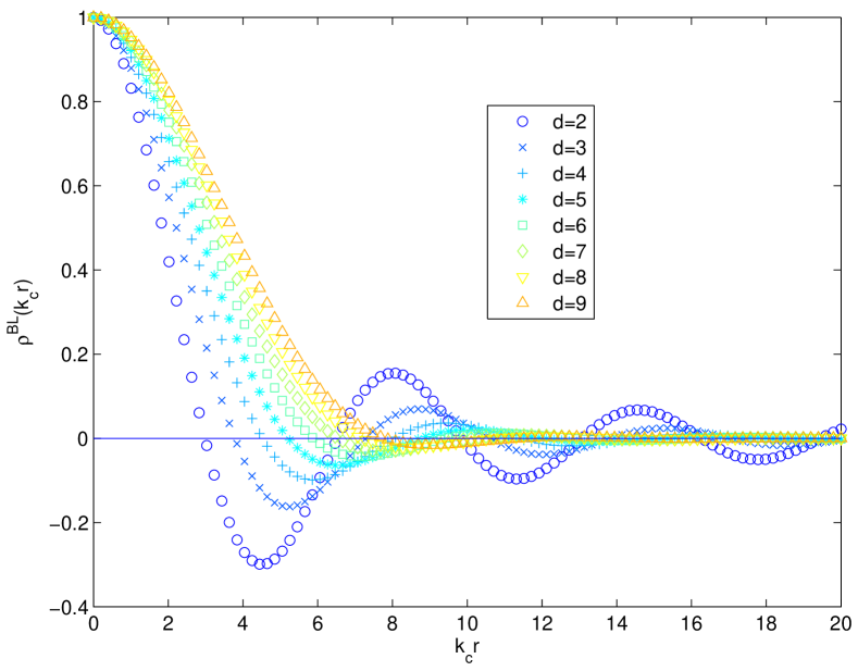
Figure 2: Dependence of the Bessel-Lommel autocorrelation function (16) on the spatial lag and $d$. The values of the parameters are $\eta_{0}=1$, $\xi=1$, ${\eta_{1}}=2$, and ${k_{c}}=2$.

The dependence of $\rho_{\rm xx}^{BL}(z;{\bm{\theta}}^{\prime})$ on $d$ is shown in Fig. 2. The amplitude of the negative peak of $C_{{\rm x}{\rm x}}^{BL}(r;{\bm{\theta}})$ diminishes with increasing $d$, whereas the lowest positive root of $C_{{\rm x}{\rm x}}^{BL}(r;{\bm{\theta}})$ moves to higher values.

VI Length Scales of SSRF and Bessel-Lommel Random Fields

In two-parameter covariance models, e.g. the Gaussian, $C_{{\rm x}{\rm x}}(r)=\sigma^{2}\,\exp(-r^{2}/\xi^{2})$ and exponential, $C_{{\rm x}{\rm x}}(r)=\sigma^{2}\,\exp(-r/\xi)$ models, all the SRF length scales are determined by $\xi$. Models with more than two parameters, such as the SSRF, Matérn, and rational quadratic, exhibit more complex dependence since their length scales are not uniquely determined by $\xi$ [54].

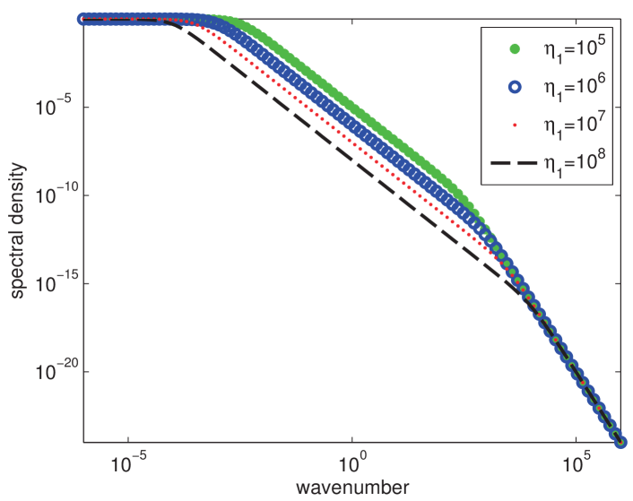
The SSRF spectral density exhibits power-law dependence over a wide range of wavevectors if ${\eta_{1}}\gg 1$; in particular, $\widetilde{C_{{\rm x}{\rm x}}}({\bf k};{\bm{\theta}})\propto k^{-2}$ for $k_{\min}<<k<k_{\max}$ where $k_{\min}=1/(\sqrt{{\eta_{1}}}\xi)$ and $k_{\max}=\sqrt{{\eta_{1}}}/\xi$. In Fig. 3 we show plots of the SSRF spectral density for ${\eta_{1}}\gg 1$, which clearly exhibit the scaling (self-similar) range with an exponent equal to $-2$ over an extensive (but still finite) range. Note that if the scaling dependence $\widetilde{C_{{\rm x}{\rm x}}}({\bf k};{\bm{\theta}})\propto k^{-2}$ persisted for all $k\gg k_{\min}$ the spectral density would not be summable.

In the Bessel-Lommel case, a necessary condition for self-similar scaling is $k_{\max}<{k_{c}}.$ As we show below, however, the Bessel-Lommel integral range declines with ${k_{c}}\uparrow$. This implies that the wide spectral band necessary to observe the scaling regime reduces spatial coherence. Hence, the regime of self-similarity is not interesting in the Bessel-Lommel case.

Figure 3: Log-log plot of SSRF spectral density for $\eta_{0}=1$, $\xi=1$, and ${\eta_{1}}=10^{5},10^{6},10^{7},10^{8}$.

VI-A Integral Range

The integral range represents a measure of the distance over which two field values are correlated [34, 54]. It is defined by the following volume integral

$$\ell_{c}=\left[\frac{\int d{\bf r}\,C_{{\rm x}{\rm x}}(r;{\bm{\theta}})}{C_{{\rm x}{\rm x}}(0;{\bm{\theta}})}\right]^{1/d}=\left(\frac{\widetilde{C_{{\rm x}{\rm x}}}(k=0;{\bm{\theta}})}{\int_{\mathbb{R}^{d}}d{\bf k}\,\widetilde{C_{{\rm x}{\rm x}}}(k;{\bm{\theta}})}\right)^{1/d}.$$ (17)

VI-A1 SSRF Covariance

For SSRF covariance functions in $\mathbb{R}^{2}$ is $\ell_{c}=A_{2}({\eta_{1}})\,\xi$ where $A_{2}({\eta_{1}})$ is a monotonically increasing function of ${\eta_{1}}$ given by equations (20)-(22) in [54].

VI-A2 Bessel-Lommel Covariance

The integral range of the covariance function $C_{{\rm x}{\rm x}}^{BL}(z;{\bm{\theta}})$ is given according to (17) by the following expression

$$\ell_{c}= \left(\frac{\widetilde{C_{{\rm x}{\rm x}}^{BL}}(k=0;{\bm{\theta}})}{C_{{\rm x}{\rm x}}^{BL}(0;{\bm{\theta}})}\right)^{1/d}=\frac{\pi^{1/2}\,2^{1-1/d}}{{k_{c}}}\,[\Gamma(d/2)]^{1/d}$$

$$\quad\cdot\left(\frac{1}{d}+{\eta_{1}}\,\frac{({k_{c}}\xi)^{2}}{d+2}+\frac{({k_{c}}\xi)^{4}}{d+4}\right)^{-1/d}.$$ (18)

We derive (VI-A2) using (11) for $\widetilde{C_{{\rm x}{\rm x}}^{BL}}(k=0;{\bm{\theta}})=(\eta_{0}\,\xi^{d})^{-1}$ and (V-C) for $C_{{\rm x}{\rm x}}^{BL}(z=0;{\bm{\theta}}).$

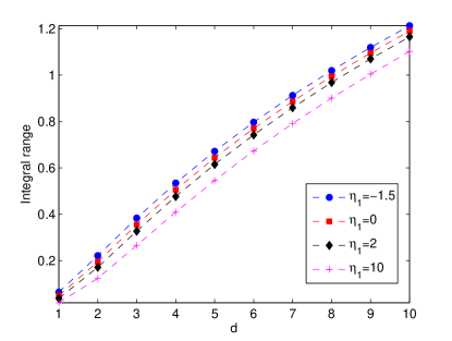
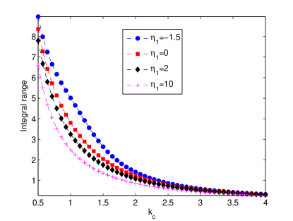
As evidenced in the parametric curves of Fig. 4a, $\ell_{c}$ increases with $d$ reflecting the concomitant suppression of the oscillations (see Fig. 2). In addition, $\ell_{c}$ decreases with increasing $\xi$ and ${\eta_{1}}.$ The reason is the steeper increase of $\widetilde{C_{{\rm x}{\rm x}}^{BL}}(k;{\bm{\theta}})$ with $k$ as $\xi\uparrow$ or ${\eta_{1}}\uparrow$, which enhances spatial variability and reduces the SRF coherence. The above trend is opposite to that of the SSRF integral range. The dependence of $\ell_{c}$ on $\xi$ enters (VI-A2) only through the product ${k_{c}}\xi=u_{c}$. Hence, for fixed $u_{c}$, $d$ and ${\eta_{1}}$, it follows from (VI-A2) that $\ell_{c}\propto 1/{k_{c}}$ as shown in  Fig. 4b. The observed decline occurs because ${k_{c}}\uparrow$ signifies a wider spectral band with increasing weight at its tail which reduces spatial coherence. The relation $\ell_{c}\propto 1/{k_{c}}$ is justified by the fact that $C_{{\rm x}{\rm x}}^{BL}(z;{\bm{\theta}})$ is a function of $z=u_{c}\,h={k_{c}}r$, which implies that the characteristic distance scale is $\propto 1/{k_{c}}$ instead of $\xi.$

(a) Integral range vs. $d$

(b) Integral range vs. ${k_{c}}$

Figure 4: (a) Integral range $\ell_{c}$ versus $d$ based on (VI-A2). (b) Integral range $\ell_{c}$ versus ${k_{c}}$ ${\eta_{1}}$ based on (VI-A2); in both cases $\xi=2$.

VI-B Correlation Spectrum

The reference [55] introduces the concept of the smoothness microscale. The microscale denotes a length such that the SRF appears smooth and can be linearly interpolated at smaller length scales. The microscale is equivalent to the integral range of the gradient of $X({\bf s},\omega)$. We extend the definition in [55] to a correlation spectrum which applies to stationary, but not necessarily mean-square differentiable SRFs with unimodal, radially symmetric spectral density.

Definition VI.1.

Let the radial function $\mathbb{R}^{d}\supset{\bf k}\mapsto\widetilde{C_{{\rm x}{\rm x}}}(k;{\bm{\theta}})$ be a permissible spectral density for a statistically isotropic SRF $X({\bf s},\omega)$ that satisfies Bochner’s theorem II.1. In addition, let $\widetilde{C_{{\rm x}{\rm x}}}(k;{\bm{\theta}})$ be a unimodal function of $k$. Then, we define the following correlation spectrum $\lambda_{c}^{(\alpha)}$ indexed by $0\leq\alpha\leq 1$

$$\lambda_{c}^{(\alpha)}= \left(\frac{\sup_{{\bf k}\in\mathbb{R}^{d}}\,k^{2\alpha}\,\widetilde{C_{{\rm x}{\rm x}}}(k;{\bm{\theta}})}{\int_{\mathbb{R}^{d}}d{\bf k}\,k^{2\alpha}\,\widetilde{C_{{\rm x}{\rm x}}}(k;{\bm{\theta}})}\;\right)^{1/d}.$$ (19)

For $\alpha=0$ the integral range (17) is recovered if the peak of the spectral density occurs at $k=0.$ If the spectral density reaches a maximum at wavenumber $k_{\max}>0$, then (19) represents approximately the width of the maximum of the spectral density.

For $\alpha=1$ the smoothness microscale is recovered. The definition of the microscale involves in the denominator of (19) the Laplacian of the covariance function evaluated at zero lag, $-[\nabla^{2}C_{{\rm x}{\rm x}}(r)]_{r=0}$. If the SRF is differentiable in the mean square sense $-[\nabla^{2}C_{{\rm x}{\rm x}}(r)]_{r=0}\in\mathbb{R}_{+}$, and thus $\lambda_{c}^{(\alpha=1)}\in\mathbb{R}_{+}$; in contrast, $[\nabla^{2}C_{{\rm x}{\rm x}}(r)]_{r=0}$ diverges for non-differentiable SRFs leading to $\lambda_{c}^{(\alpha=1)}=0$. The zero microscale denotes that the SRF appears rough at all length scales.

Exponents $0<\alpha<1$ generate a spectrum of scales which emphasizes different parts of the spectral density. Correlation lengths obtained for $0<\alpha<1$ correspond to the integral range of the SRF’s fractional derivative of order $\alpha$. Based on (19) these length scales involve the fractional Laplacian of the covariance function [56] at zero lag, and they take finite, non-zero values if $k^{2\alpha}\,\widetilde{C_{{\rm x}{\rm x}}}(k;{\bm{\theta}})$ is integrable. A necessary condition for integrability is that $\widetilde{C_{{\rm x}{\rm x}}}(k;{\bm{\theta}})\underset{k\rightarrow\infty}{\sim}k^{-q}$ where $q>2\alpha+d$. Hence, for fixed $q$ a non-vanishing length scale is obtained for $\alpha<\alpha_{\max}=(q-d)/2$; thus, the respective length scales $\lambda_{c}^{(\alpha)}$ can be used to quantify the “fractional smoothness” of continuous but non-differentiable random fields.

VI-B1 SSRF Covariance

For $\alpha=1$, it follows from (19) that $\lambda_{c}^{(\alpha)}=0$, because the integral in the denominator develops a logarithmic divergence marking the non-existence of the covariance Laplacian at zero. The loss of mean square differentiability implies that the smoothness microscale is zero regardless of ${\eta_{1}}$ and $\xi$. The failure of the microscale to discriminate between different SSRF parameters is unsatisfactory, since the latter affect the small-scale structure of field realizations as evidenced in the plots shown in Fig. 7 below.

For $0\leq\alpha<1$, however, $\lambda_{c}^{(\alpha)}>0$; in addition, $\lambda_{c}^{(\alpha)}$ depends on the SSRF parameters. Hence, $\lambda_{c}^{(1-\epsilon)}$ where $0<\epsilon\ll 1$ distinguishes between different SSRF covariance models.

Proposition 3.

The correlation spectrum for the SSRF covariance functions with spectral density (5) are given by the following equation in $3\geq d\geq 1$

$$\lambda_{c}^{(\alpha)}= \xi\,\left(\frac{(\tilde{\kappa}_{1}\,\xi)^{2\alpha}\Big{/}b(\alpha,{\eta_{1}})}{1+{\eta_{1}}(\tilde{\kappa}_{1}\xi)^{2}+(\tilde{\kappa}_{1}\xi)^{4}}\right)^{1/d},$$ (20)

where

$$b(\alpha,{\eta_{1}}) =\left\{\begin{array}[]{cc}\frac{\pi\,\Gamma(1-\alpha)\Gamma(1+\alpha)\,\left[\left({\eta_{1}}+\Delta\right)^{\alpha}-\left({\eta_{1}}-\Delta\right)^{\alpha}\right]}{2^{\alpha}\alpha\Delta}&{\eta_{1}}\neq 2\\ \pi\,\Gamma(1+\alpha)\,\Gamma(1-\alpha)&{\eta_{1}}=2\end{array}\right.$$ (23)

$\Delta=\sqrt{{\eta_{1}}^{2}-4}$, and $\tilde{\kappa}_{1}=\underset{{k}}{\arg\max}\left(k^{2\alpha}\,\widetilde{C_{{\rm x}{\rm x}}}(k;{\bm{\theta}})\right)$, i.e.,

$$\tilde{\kappa}_{1}=\sqrt{\frac{\sqrt{{\eta_{1}}^{2}\,(1-\alpha)^{2}-4\alpha(\alpha-2)}-{\eta_{1}}\,(1-\alpha)}{2(2-\alpha)\xi^{2}}}.$$ (24)

Proof:

The proof is given in the Appendix C. ∎

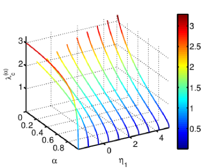
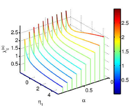
The dependence of $\lambda_{c}^{(\alpha)}$ on ${\eta_{1}}$ and $\alpha$ is shown in Fig. 5. The general trend, as shown in Fig. 5a, is that $\lambda_{c}^{(\alpha)}\downarrow$ as $\alpha\uparrow$, leading to $\lambda_{c}^{(1)}=0$ which marks the SSRF non-differentiability. The decline of $\lambda_{c}^{(\alpha)}$ with $\alpha\uparrow$ reflects the fact that higher $\alpha$ emphasize shorter length scales (wavelenghts) as marked by the increase of $\tilde{\kappa}_{1}$ with $\alpha$ at fixed ${\eta_{1}}$. The curves in Fig. 5b show that for $\alpha>\alpha_{\min}\approx 2$, $\lambda_{c}^{(\alpha)}\downarrow$ as ${\eta_{1}}\uparrow$, indicating that higher rigidity reduces the fine-scale regularity of the field. For $\alpha\leq\alpha_{\min}$, i.e., for coarser scales, first $\lambda_{c}^{(\alpha)}\downarrow$ for ${\eta_{1}}\lessapprox-1$, and then $\lambda_{c}^{(\alpha)}\uparrow$ as ${\eta_{1}}\uparrow$ beyond ${\eta_{1}}\gtrapprox-1$.

(a) SSRF scales - fixed ${\eta_{1}}$

(b) SSRF scales - fixed $\alpha$

Figure 5: SSRF correlation spectrum (20) versus ${\eta_{1}}\in[-1.9,5]$ and $\alpha\in[0,1]$ for $\xi=5$ and $d=2$. (a) Continuous lines correspond to curves of fixed ${\eta_{1}}$. The curves displayed are for ten evenly spaced ${\eta_{1}}$ values between $-1.9$ to $5$ (from left to right in the plot). (b) Continuous lines correspond to curves of fixed $\alpha$. The curves displayed are for ten evenly spaced $\alpha$ values between $0.05$ to $0.95$ (from right to left in the plot).

VI-B2 Bessel-Lommel Covariance

Proposition 4.

The correlation spectrum for the Bessel-Lommel covariance functions with spectral density (11) are given by the following equation in $d\geq 2$

$$\lambda_{c}^{(\alpha)} =\frac{g_{d}}{{k_{c}}}\left(1+{\eta_{1}}\tilde{{k_{c}}}^{2}+\tilde{{k_{c}}}^{4}\right)^{1/d},\;{\eta_{1}}>{\eta_{1,c}}\lor{k_{c}}<\kappa_{-}$$ (25a)

$$\lambda_{c}^{(\alpha)} =\frac{g_{d}}{{k_{c}}}\left(1+{\eta_{1}}\tilde{\kappa}_{-}^{2}+\tilde{\kappa}_{-}^{4}\right)^{1/d},\;{\eta_{1,c}}\geq{\eta_{1}}>-2$$

$$\hskip 108.405pt\wedge\kappa_{+}\geq{k_{c}}>\kappa_{-},$$ (25b)

$$\lambda_{c}^{(\alpha)} =\frac{g_{d}}{{k_{c}}}\left(1+{\eta_{1}}(\tilde{\kappa}^{\ast})^{2}+(\tilde{\kappa}^{\ast})^{4}\right)^{1/d},\;{\eta_{1,c}}\geq{\eta_{1}}>-2$$

$$\hskip 115.63243pt\wedge{k_{c}}>\kappa_{+},$$ (25c)

where $\tilde{{k_{c}}}={k_{c}}\xi$, $\tilde{\kappa}_{-}={\kappa}_{-}\xi$, $\tilde{\kappa}^{\ast}={\kappa}^{\ast}\xi$,

$${\eta_{1,c}}=-\frac{2\,\sqrt{\alpha(\alpha+2)}}{(\alpha+1)},$$ (26a)

$$g_{d}=\left[\frac{\Gamma(d/2)}{2\,\pi^{d/2}\,\left(\frac{1}{d+2\alpha}+\frac{{\eta_{1}}\,{k_{c}}^{2}\,\xi^{2}}{d+2\alpha+2}+\frac{{k_{c}}^{4}\,\xi^{4}}{d+2\alpha+4}\right)}\right]^{1/d},$$ (26b)

$$\kappa_{\pm}=\frac{1}{\xi}\sqrt{\frac{-(\alpha+1){\eta_{1}}\pm\sqrt{(\alpha+1)^{2}{\eta_{1}}^{2}-4\alpha(\alpha+2)}}{2(\alpha+2)}},$$ (26c)

and $\kappa^{\ast}=\arg\max\left(\kappa_{-}^{2\alpha}\,\Pi(\kappa_{-}\xi),{k_{c}}^{2\alpha}\,\Pi({k_{c}}\xi)\right)$, $\Pi(x)$ being the polynomial defined in (5b).

Proof:

The proof is given in the Appendix D. ∎

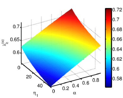
The dependence of $\lambda_{c}^{(\alpha)}$ on ${\eta_{1}},\alpha,{k_{c}}$ is shown in Fig. 6. Overall, higher ${\eta_{1}}$ and ${k_{c}}$ tend to reduce $\lambda_{c}^{(\alpha)}$. The ${k_{c}}$ dependence is more pronounced and follows asymptotically $\lambda_{c}^{(\alpha)}\sim 1/{k_{c}}^{3}$. The increase of $\lambda_{c}^{(\alpha)}$ with $\alpha$ signifies that the smoothness microscale exceeds the integral range. This effect is due on one hand to the high smoothness of the B-L random field that increases the microscale and on the other to the oscillations of the B-L covariance function which reduce the integral range.

(a) BL scales $\xi=5,{k_{c}}=\pi/2$

(b) BL scales ${\eta_{1}}=3,\xi=5$

Figure 6: Spectrum of Bessel-Lommel correlation scales in $d=2$. (a) $\lambda_{c}^{(\alpha)}$ for ${\eta_{1}}\in[0,50]$ and $\alpha\in[0,1]$ with $\xi=5,{k_{c}}=\pi/2$. (b) $\lambda_{c}^{(\alpha)}$ for ${k_{c}}\in[0.1,5]$ and $\alpha\in[0,1]$ with ${\eta_{1}}=3,\xi=5$.

VII Simulations

We present realizations of SRFs with SSRF and Bessel-Lommel correlation structures. The spectral simulation method based on the Fast Fourier Transform (FFT) [57, 55, 58] is used to generate the realizations on square grids of length $L=512$.

VII-A Random Fields with SSRF Covariance

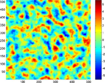
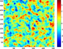
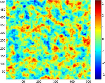
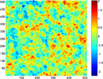
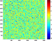
Four different SSRF realizations are shown in Fig. 7. The realizations correspond to fields with common $\eta_{0}$ and $\xi$ but different $\eta_{1}$. The patterns become “grainier” as $\eta_{1}$ increases. Nevertheless, the integral range $\ell_{c}$ increases with $\eta_{1}$, as discussed in section VI-A1.

(a) $\eta_{1}=-1.5$

(b) $\eta_{1}=0$

(c) $\eta_{1}=1.5$

(d) $\eta_{1}=15$

Figure 7: SSRF realizations with covariance function (8) on a square $512\times 512$ grid. For all realizations $\eta_{0}=10,\xi=10$. FFT spectral simulation with the same random generator seed is used in all the simulations.

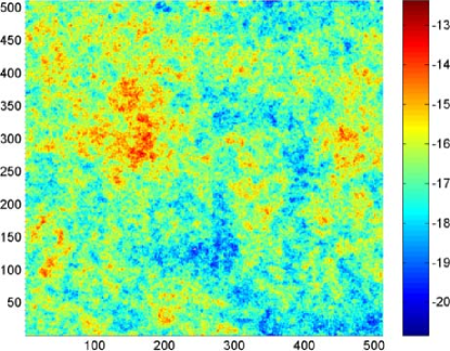
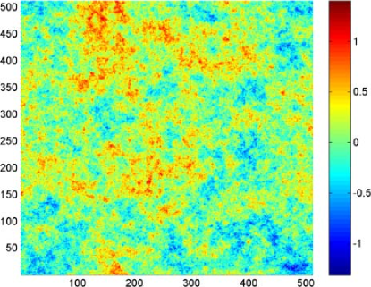
Two realizations with ${\eta_{1}}\gg 1$ that exhibit multiscaling are shown in Fig. 8. For ${\eta_{1}}\gg 1$ it follows from [54, eq. (22)] that $r_{c}\approx\xi\sqrt{2\pi\,{\eta_{1}}/\log{\eta_{1}}}$. Hence, the realization shown in Fig. 8a is drawn from a field with $r_{c}\approx 2336$, whereas the one shown in Fig. 8b corresponds to $r_{c}\approx 6743$. In both cases the domain size does not allow adequate sampling of the probability distribution. This non-ergodic effect is responsible for the difference in the range of field values between the two plots. The lack of ergodicity is more pronounced in Fig. 8b, where all the field values are negative (see vertical scale bar).

(a) $\eta_{0}=10^{4},{\eta_{1}}=10^{5},\xi=10$

(b) $\eta_{0}=10^{6},{\eta_{1}}=10^{6},\xi=10$

Figure 8: Multiscale SSRF realizations with covariance function (8) on square $512\times 512$ grid. (a): $\eta_{0}=10^{4},{\eta_{1}}=10^{5},\xi=10$; (b): $\eta_{0}=10^{6},{\eta_{1}}=10^{6},\xi=10$. FFT spectral simulation with clock dependent random generator seed is used.

VII-B Random Fields with Bessel-Lommel Covariance

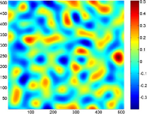
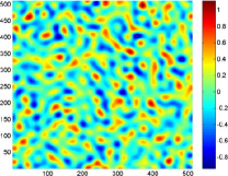
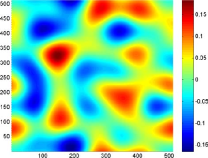
Four different realizations of Bessel-Lommel SRFs are shown in Fig. 9. The realizations have identical $\eta_{0}$, $\eta_{1}$ and $\xi$ but different ${k_{c}}$. Two trends are obvious in the plots: (i) the variance of the fluctuations increases with ${k_{c}}$ and (ii) the size of characteristic spatial patterns (i.e., areas containing values above or below a given threshold) is reduced as ${k_{c}}$ increases. Trend (i) is due to increased spectral weight in the tail of the spectral density function (11) as ${k_{c}}\uparrow$. Trend (ii) reflects the decline of the integral range with ${k_{c}}\uparrow$ according to (VI-A2) and as shown in Fig. 6b.

(a) ${k_{c}}=0.05$

(b) ${k_{c}}=0.1$

(c) ${k_{c}}=0.2$

(d) ${k_{c}}=0.5$

Figure 9: Bessel-Lommel SRF realizations with covariance function (8) on square $512\times 512$ grid. For all realizations $\eta_{0}=0.01,\eta_{1}=1,\xi=2$. FFT spectral simulation with identical random generator seed is used.

VIII Results, Discussion and Conclusions

The main results of this paper consist of Propositions 1-4 and Definition VI.1. More specifically, we introduce covariance functions with enhanced parametric dependence motivated by local interaction SRF models. We derive explicit expressions (8c) for two-dimensional, three-parameter, radial SSRF covariance functions at the limit of infinite spectral cutoff. Gaussian SRFs with such covariance functions are continuous but non-differentiable in the mean square sense.

In addition to SSRF covariance functions, we develop a family of four-parameter, radial Bessel-Lommel covariance functions (14) that are valid in $d\geq 2$. In contrast with their SSRF counterparts, the Bessel-Lommel functions are infinitely differentiable at the origin, signifying that a Gaussian SRF with such covariance dependence is infinitely differentiable in the mean square sense.

Since covariance functions are the key ingredient in best linear unbiased estimation methods, e.g., kriging [33, 24], the SSRF and Bessel-Lommel functions will provide increased flexibility in the interpolation and simulation of spatial processes [15, 32, 33]. In addition, they can be used as background error covariance models in variational assimilation of geophysical data [59, 60]. They also provide new choices of radial functions suitable for applications in radial basis function interpolation [38]. Finally, they constitute non-negative definite kernel functions with potential for applications in machine learning [45].

We also demonstrate that the length scales of SRFs with SSRF and Bessel-Lommel covariance functions are not uniquely determined by a single characteristic length $\xi$. We illustrate this behavior by investigating the integral range of the above covariance models. In addition, we introduce a correlation spectrum based on the Fourier transform of the covariance function’s fractional Laplacian of order $0\leq\alpha\leq 1$. This spectrum allows quantifying correlation properties of mean-square continuous SRFs with a radial, unimodal spectral density. Finally, we derive explicit expressions for the $\alpha$-spectrum of SSRF and Bessel-Lommel covariance functions.

The assumption of statistical isotropy was used herein primarily for reasons of conciseness in presentation. Nonetheless, it is straightforward to construct covariance models with geometric (elliptic) anisotropy by rotation and rescaling transformations of the coordinate axes [61, 62, 63].

Appendix A Proof of Proposition 1

Proof:

Defining dimensionless wavevectors $u=k\,\xi$ and lag distances $h=r/\xi$, the spectral integral (7) is simplified as follows:

$$C_{{\rm x}{\rm x}}(h;{\bm{\theta}})=\frac{\eta_{0}}{2\pi}\,\int\limits_{0}^{\infty}du\,\frac{u\,J_{0}(u\,h)}{1+{\eta_{1}}u^{2}+u^{4}}.$$ (A-1)

Equation (A-1) shows that the only non-trivial parameter is ${\eta_{1}}$; $\eta_{0}$ is a multiplicative scale factor, whereas the characteristic length $\xi$ is absorbed in the non-dimensional lag $h.$ The rational function $1/\Pi(u)$, where $\Pi(u)$ is the SSRF characteristic polynomial defined in (5b), admits the following expansion

$$\frac{1}{\Pi(u)}=\left\{\begin{array}[]{cc}\frac{1}{t_{+}^{\ast}-t_{-}^{\ast}}\,\left(\frac{1}{u^{2}-t_{+}^{\ast}}-\frac{1}{u^{2}-t_{-}^{\ast}}\right),&{\eta_{1}}\neq 2\\ \frac{1}{(u^{2}+1)^{2}}&{\eta_{1}}=2,\end{array}\right.$$ (A-2)

where $t_{\pm}^{\ast}={\left(-{\eta_{1}}\pm\Delta\right)}/{2}$ are the roots of $\Pi(t=u^{2})$.

In light of (A-2), the integral (A-1) is evaluated using the Hankel-Nicholson formula (11.4.44) in [51, p. 364]:

$$\int_{0}^{\infty}du\frac{u^{\nu+1}J_{\nu}(h\,u)}{(u^{2}+z^{2})^{\mu+1}}=\frac{h^{\mu}z^{\nu-\mu}}{2^{\mu}\Gamma(\mu+1)}K_{\nu-\mu}(h\,z).$$ (A-3)

This equation is valid for $h>0,\Re(z)>0$, and $-1<\Re(\nu)<2\Re(\mu)+\frac{3}{2}$. The above is applied to (A-1) with (i) ${\eta_{1}}\neq 2$, $\nu=0$, $\mu=0$,   $z^{2}_{\pm}=-t_{\pm}^{\ast}$ and (ii) ${\eta_{1}}=2$, $\nu=0$ and $\mu=1$. In case (ii) we obtain (8b) and in case (i) the following

$$C_{{\rm x}{\rm x}}(h;{\bm{\theta}})=\frac{\eta_{0}\left[K_{0}(hz_{+})-K_{0}(hz_{-})\right]}{2\pi\sqrt{\eta_{1}^{2}-4}},\;{\eta_{1}}\neq 2.$$

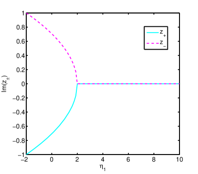
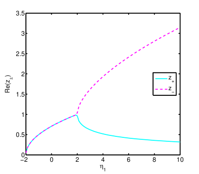
The coefficients $z_{\pm}=\sqrt{-t_{\pm}^{\ast}}$ are plotted versus ${\eta_{1}}$ in Fig. 10. For ${\eta_{1}}>2$ both $z_{+}$ and $z_{-}$ are real numbers, hence proving (8a). For $-2<{\eta_{1}}<2$ $\Re(z_{+})=\Re(z_{-})$, whereas $\Im(z_{+})=-\Im(z_{-})$, i.e., $z_{-}=\overline{z_{+}}$. The analytic continuation property $K_{0}(\overline{z})=\overline{K_{0}(z)}$ [51, p. 377] leads to (8c) which is explicitly real-valued.

A-1 Continuity

A stationary SRF is mean square continuous $\forall{\bf s}\in\mathbb{R}^{d}$ if and only if its covariance function is continuous at zero lag  [1, 64]. This condition is satisfied for the SSRF covariance.

A-2 Differentiability

Differentiability of the SRF $X({\bf s},\omega)$ in the mean-square sense requires that all second-order partial derivatives of the covariance function at $\|{\bf r}\|=0$ exist [1, p. 27]. This requirement is equivalent to the convergence of the second-order spectral moment

$$\Lambda_{d}^{(2)}:=\int_{\mathbb{R}^{d}}d{\bf k}\,k^{2}\,\widetilde{C_{{\rm x}{\rm x}}}({\bf k},{\bm{\theta}}).$$

For the SSRF spectral density in $d=2$ the above becomes

$$\Lambda_{2}^{(2)}\propto\lim_{{k_{c}}\rightarrow\infty}\int_{0}^{{k_{c}}}dk\,\frac{k^{3}}{1+{\eta_{1}}(k\xi)^{2}+(k\xi)^{4}}.$$

This integral develops a logarithmic divergence as ${k_{c}}\rightarrow\infty$. Hence, the SSRF is non-differentiable in the mean-square sense.

(a) Real part of $z_{\pm}=\sqrt{-t_{\pm}^{\ast}}$

(b) Imaginary part of $z_{\pm}=\sqrt{-t_{\pm}^{\ast}}$

Figure 10: Real and imaginary parts of the roots $z_{+}=\sqrt{-t_{+}^{\ast}}$ and $z_{-}=\sqrt{-t_{-}^{\ast}}$ of the characteristic polynomial $\Pi(u)=1+\eta_{1}u^{2}+u^{4}$ according to (9).

∎

Appendix B Proof of Proposition 2

Proof:

Let $z=u_{c}\,h$, $\nu=d/2-1$, $\mu>-(\nu+1)$, and $J_{\nu}(\cdot)$ be the Bessel function of the first kind of order $\nu$. We then define the function

$$\mathcal{A}_{\mu,\nu}(z)=\int_{0}^{1}dx\,x^{\mu}J_{\nu}(z\,x).$$ (B-1)

Then, $\mathcal{A}_{\mu,\nu}(z)$ is evaluated using [65, p. 676, eq. (6.561.13)] as follows

$$\mathcal{A}_{\mu,\nu}(z)= \frac{2^{\mu}\Gamma\left(\frac{\nu+\mu+1}{2}\right)}{z^{\mu+1}\,\Gamma\left(\frac{\nu-\mu+1}{2}\right)}+\frac{(\mu+\nu-1)J_{\nu}(z)S_{\mu-1,\nu-1}(z)}{z^{\mu}}$$

$$\quad\quad\quad-\frac{J_{\nu-1}(z)S_{\mu,\nu}(z)}{z^{\mu}}.$$ (B-2)

We use the normalizing variable transformations $x=k/{k_{c}}$, $h=r/\xi,$ and $u_{c}={k_{c}}\xi$. In view of the dimensionless variables $x,h,u_{c}$, the integral (10) becomes

$$C_{{\rm x}{\rm x}}^{BL}(h;{\bm{\theta}})= \frac{u_{c}^{1+d/2}\,h^{1-d/2}}{(2\pi)^{d/2}\eta_{0}\,\xi^{2d}}\int_{0}^{1}dx\,{x^{d/2}J_{d/2-1}(xhu_{c})}$$

$$\quad\cdot\left[1+{\eta_{1}}(xu_{c})^{2}+(xu_{c})^{4}\right].$$ (B-3)

In light of (B-1), (B) and using $z=u_{c}h={k_{c}}r$ as the dimensionless distance, the function $C_{{\rm x}{\rm x}}^{BL}({\bf r};{\bm{\theta}})$ defined by (10) is given by

$$C_{{\rm x}{\rm x}}^{BL}(z;{\bm{\theta}})= \frac{g_{0}({\bm{\theta}})}{z^{\nu}}\left[\mathcal{A}_{\nu+1,\nu}(z)+{\eta_{1}}u_{c}^{2}\mathcal{A}_{\nu+3,\nu}(z)\right.$$

$$\left.\quad\quad\quad+u_{c}^{4}\mathcal{A}_{\nu+5,\nu}(z)\right],$$ (B-4)

$$g_{0}({\bm{\theta}})=\frac{{k_{c}}^{d}}{(2\pi)^{d/2}\eta_{0}\,\xi^{d}}.$$ (B-5)

For the three terms $\mathcal{A}_{\mu,\nu}(z)$ $(\mu=\nu+1,\nu+3,\nu+5)$ included in $C_{{\rm x}{\rm x}}^{BL}(z;{\bm{\theta}})$, the parameters $\mu,\nu$ satisfy the relation

$$\nu-\mu+1=-2\,l,\;\mbox{where}\;l=0,1,2.$$ (B-6)

Equations (14) follow directly from (B) which expresses $C_{{\rm x}{\rm x}}^{BL}(z;{\bm{\theta}})$ in terms of $\mathcal{A}_{\mu,\nu}(z)$, and from (B) which expresses the integrals $\mathcal{A}_{\mu,\nu}(z)$ in terms of Lommel functions. In view of (B-6), the Gamma function contributions to $\mathcal{A}_{\nu+2l+1,\nu}(z)$ in (B) vanish due to the poles of $\Gamma(n)$ at $n\in\mathbb{Z}_{0,-}$.

B-1 Permissibility

The non-negative definiteness of $C_{{\rm x}{\rm x}}^{BL}(z;{\bm{\theta}})$ is based on Bochner’s theorem and the fact that, according to (11), $\widetilde{C_{{\rm x}{\rm x}}^{BL}}(k;{\bm{\theta}})\geq 0$ for ${\eta_{1}}>-2$.

B-2 Differentiability

The existence of the $n$-th order partial derivatives of the Bessel-Lommel SRF in the mean-square sense requires that all the partial derivatives of order $2n$ of $C_{{\rm x}{\rm x}}^{BL}(z;{\bm{\theta}})$ exist at $z=0$. This condition is ensured by the convergence of the $2n$-th order spectral moment

$$\Lambda_{d}^{(2n)}=\int_{0}^{{k_{c}}}dk\,{k^{n+d-1}}{\,\left[1+{\eta_{1}}(k\xi)^{2}+(k\xi)^{4}\right]}.$$

∎

Appendix C Proof of Proposition 3

Proof:

To find the supremum of $f(k):=k^{2\alpha}\,\widetilde{C_{{\rm x}{\rm x}}}(k;{\bm{\theta}})$ we consider the extremum condition ${\rm d}f(k)/{\rm d}k=0$, which admits the following two roots:

$$\tilde{\kappa}_{1,2}=\sqrt{\frac{\pm\sqrt{{\eta_{1}}^{2}\,(1-\alpha)^{2}-4\alpha(\alpha-2)}-{\eta_{1}}\,(1-\alpha)}{2(2-\alpha)\xi^{2}}}.$$

For $0\leq\alpha<1$ only $\tilde{\kappa}_{1}\in\mathbb{R}$ and $\sup f(k)=f(\tilde{\kappa}_{1})$.

According to (5) the denominator of (19) becomes

$$\mathcal{S}_{d}\,\eta_{0}\,\xi^{1-2\alpha}\,\int_{0}^{\infty}dx\,\phi_{\alpha}(x)$$ (C-1)

$$\mbox{where}\quad\phi_{\alpha}(x)= \frac{x^{1+2\alpha}}{1+{\eta_{1}}\,\xi^{2}\,x^{2}+\xi^{4}\,x^{4}}.$$ (C-2)

To simplify notation we define

$$I_{\alpha}(\phi):=\int_{0}^{\infty}dx\phi_{\alpha}(x).$$ (C-3)

In order to calculate the integral (C-1) we use Lebesgue’s dominated convergence theorem [53] expressed as follows:

Theorem C.1.

Let $\phi_{\alpha}(x)$ be a real-valued function $\forall x\in\mathbb{R}$ which is integrable $\forall\alpha\in[0,1]$. If there is a real-valued function $g_{n}(x)$ such that (i) $\lim_{n\rightarrow\infty}\phi_{\alpha}(x)\,g_{n}(x)=\phi_{\alpha}(x),\,\forall x\in\mathbb{R}$ and (ii) $|\phi_{\alpha}(x)\,g_{n}(x)|\leq\phi^{\ast}(x),\forall x\in\mathbb{R}$, where $\phi^{\ast}(x)$ is an integrable function, then

$$I_{\alpha}(\phi) =\int_{0}^{\infty}dx\lim_{n\rightarrow\infty}g_{n}(x)\phi_{\alpha}(x)=\lim_{n\rightarrow\infty}\int_{0}^{\infty}dxg_{n}(x)\phi_{\alpha}(x).$$

We define the following auxiliary function

$$g_{n}(x):=\frac{2^{\alpha}\,\Gamma(\alpha+1)\,J_{\alpha}(x/n)}{\left(\frac{x}{n}\right)^{\alpha}}.$$ (C-4)

Condition (i) of Theorem C.1 is satisfied because $\lim_{n\rightarrow\infty}g_{n}(x)=1$ based on the infinite series expansion of the Bessel function of the first kind around zero [52, p. 40].

To prove the condition (ii) we apply the following steps.

1. For condition (ii) it suffices that $|\phi_{\alpha}(x)\,g_{n}(x)|\leq\phi_{\alpha}(x)$, because $\phi_{\alpha}(x)$ given by (C-2) is integrable. Given that $\phi_{\alpha}(x)>0$, it suffices to show that $|g_{n}(x)|\leq 1$.

2. We use the integral representation of $J_{\alpha}(z)$ given by [65, 8.411.4], where $z\in\mathbb{R}$:

   $$J_{\alpha}(z)=\frac{2\left(\frac{z}{2}\right)^{\alpha}}{\Gamma(\alpha+1/2)\Gamma(1/2)}\,\int_{0}^{\pi/2}d\theta\sin^{2\alpha}\theta\cos\left(z\cos\theta\right)$$

3. Since $|\sin^{2\alpha}(\theta)\cos\left(z\cos\theta\right)|\leq 1$ and $\Gamma(1/2)=\sqrt{\pi}$ it follows from the above that $|J_{\alpha}(z)|\leq\frac{\left(\frac{z}{2}\right)^{\alpha}\sqrt{\pi}}{\Gamma(\alpha+1/2)}.$

4. In light of this inequality and (C-4), proving that $|g_{n}(x)|\leq 1$ is equivalent to showing that $\mu_{\alpha}:=\Gamma(\alpha+1)/\Gamma(\alpha+1/2)\leq\sqrt{\pi}.$

5. Based on the inequality $\mu_{\alpha}<\sqrt{\alpha+1/2}$ (valid for $\alpha>-1/4$) the maximum upper bound of $\mu_{\alpha}$ for $0\leq\alpha\leq 1$ is $\sqrt{3/2}<\sqrt{\pi}$. Hence, in light of the previous step $|g_{n}(x)|\leq 1$. This concludes the proof of condition (ii).

In light of the above, we can use dominated convergence to calculate $I_{\alpha}(\phi)$ as follows

$$I_{\alpha}(\phi)=\lim_{n\rightarrow\infty}(2n)^{\alpha}\Gamma(\alpha+1)\,\tilde{I}_{\alpha}(\phi)$$ (C-5)

where

$$\tilde{I}_{\alpha}(\phi)=\int_{0}^{\infty}dx\,\frac{J_{\alpha}(x/n)x^{1+\alpha}}{1+{\eta_{1}}\xi^{2}x^{2}+\xi^{4}x^{4}}.$$ (C-6)

The integral $\tilde{I}_{\alpha}(\phi)$ is evaluated by means of the Hankel-Nicholson formula (A-3) ($\nu=\alpha,$ $\mu=0$ for ${\eta_{1}}\neq 2$ , $\mu=1$ for ${\eta_{1}}=2$) which leads to

$$\tilde{I}_{\alpha}(\phi)=\left\{\begin{array}[]{cc}\frac{z_{+}^{\alpha}\,K_{\alpha}(z_{+}/n)-z_{-}^{\alpha}\,K_{\alpha}(z_{-}/n)}{\sqrt{{\eta_{1}}^{2}-4}}&{\eta_{1}}\neq 2\\ \frac{K_{\alpha-1}(1/n)}{2n}=\frac{K_{1-\alpha}(1/n)}{2n}&{\eta_{1}}=2.\end{array}\right.$$ (C-9)

To evaluate $\lim_{n\rightarrow\infty}\tilde{I}_{\alpha}(\phi)$ for $1>p>0$ we use the series expansion [53] of the K-Bessel function

$$K_{p}(x)= \frac{1}{2}\left[\Gamma(p)\left(\frac{2}{x}\right)^{p}\left(1+O(x^{2})\right)+\Gamma(-p)\left(\frac{x}{2}\right)^{p}\right.$$

$$\left.\quad\quad\left(1+O(x^{2})\right)\right].$$

For ${\eta_{1}}=2$, $p=1-\alpha$, and $x=1/n$ the dominant contribution at $n\rightarrow\infty$ comes from the $O(x^{-p})$ term of the first series on the right hand side, which gives $K_{1-\alpha}(1/n)\approx\frac{1}{2}\Gamma(1-\alpha)(2n)^{1-\alpha}$.

For ${\eta_{1}}\neq 2$ the $O(x^{-p})$ term of the first series cancels out due to the difference between the two Bessel functions, whereas the $O(x^{2-p})$ terms vanish at the limit $n\rightarrow\infty$. A finite contribution comes from the $O(x^{p})$ term of the second series on the right hand side, i.e., $z_{+}^{\alpha}\,K_{\alpha}(z_{+}/n)-z_{-}^{\alpha}\,K_{\alpha}(z_{-}/n)\sim\frac{\Gamma(-\alpha)}{2(2n)^{\alpha}}\left(z_{+}^{2\alpha}-z_{-}^{2\alpha}\right)$.

Thus, based on the above asymptotic analysis of the K-Bessel function, (C-5), (C-6), and (C-9) we obtain the following equation (where $\Delta=\sqrt{{\eta_{1}}^{2}-4}$):

$$I_{\alpha}(\phi)= \left\{\begin{array}[]{cc}\frac{\Gamma(1-\alpha)\Gamma(1+\alpha)\,\left[\left({\eta_{1}}+\Delta\right)^{\alpha}-\left({\eta_{1}}-\Delta\right)^{\alpha}\right]}{2^{\alpha+1}\alpha\Delta}&{\eta_{1}}\neq 2\\ \frac{\Gamma(1-\alpha)\,\Gamma(1+\alpha)}{2}&{\eta_{1}}=2.\end{array}\right.$$ (C-12)

Finally, based on (C-12), the definition (C-3) and (C-1), (20) is proved.

∎

Appendix D Proof of Proposition 4

Proof:

Based on the spectral density (11) it follows that the denominator in (19) is given by

$$\int_{\mathbb{R}^{d}}d{\bf k}\,k^{2\alpha} \widetilde{C_{{\rm x}{\rm x}}}^{BL}(k;{\bm{\theta}})=\frac{\mathcal{S}_{d}{k_{c}}^{d+2\alpha}}{\eta_{0}\xi^{d}}\left(\frac{1}{d+2\alpha}\right.$$

$$\left.+\frac{{\eta_{1}}{k_{c}}^{2}\xi^{2}}{d+2\alpha+2}+\frac{{k_{c}}^{4}\xi^{4}}{d+2\alpha+4}\right).$$ (D-1)

Let us define the function $\phi(k)=k^{2\alpha}\,\widetilde{C_{{\rm x}{\rm x}}}^{BL}(k;{\bm{\theta}})$. The numerator in (19) is then given by $\sup_{k\in\mathbb{R}}\,\phi(k)=\phi(\kappa^{\ast})$ where $\kappa^{\ast}=\underset{{k}\in[0,{k_{c}}]}{\arg\max}\phi(k)$.

D-1 Non-negative ${\eta_{1}}$

For ${\eta_{1}}\geq 0$, $\phi(k)$ is a monotonically increasing function of $k$; thus, $\kappa^{\ast}={k_{c}}$ and $\phi(\kappa^{\ast})=\frac{{k_{c}}^{2\alpha}}{\eta_{0}\xi^{d}}\,\left(1+{\eta_{1}}\,{k_{c}}^{2}\,\xi^{2}+{k_{c}}^{4}\xi^{4}\right)$. In light of (D), this leads to (25a).

D-2 Negative ${\eta_{1}}$

For ${\eta_{1}}<0$, $\phi(k)$ develops local extrema at the wavenumbers that solve the equation $d\phi(k)/dk=0$, i.e., at the $\kappa_{\pm}$ given by (26c) .

Complex $\kappa_{\pm}$

For ${\eta_{1}}^{2}<4\alpha(\alpha+2)/(\alpha+1)^{2}$, the $\kappa_{\pm}$ are complex numbers and thus $\phi(k)$ does not have local extrema for $k\in\mathbb{R}$. Hence, $\kappa^{\ast}={k_{c}}$ and $\lambda_{c}^{(\alpha)}$ is given by (25a).

Real $\kappa_{\pm}$

For $4>{\eta_{1}}^{2}\geq 4\alpha(\alpha+2)/(\alpha+1)^{2}$, the $\kappa_{\pm}$ are real numbers, one corresponding to the position of a local minimum whereas the other to a local maximum.

If $\alpha>0$, $d\phi(k)/dk\propto 2\alpha\,(k\xi)^{2\alpha-1}$ for $k\ll 1$, and thus $\phi(k)\uparrow$. Hence, the maximum of $\phi(k)$ occurs at lower $k$ than the minimum, i.e., at $\kappa_{-}<\kappa_{+}$. If $\alpha=0$, then $d\phi(k)/dk\propto-2|{\eta_{1}}|\,k\,\xi$ and thus $\phi(k)\downarrow$ for $k\ll 1$. In this case as well $\phi(k)$ reaches the maximum at $\kappa_{-}=0,$ whereas the minimum occurs at $\kappa_{+}=\sqrt{|{\eta_{1}}|/2}/({k_{c}}\xi)$. Again, we distinguish between two cases:

1. If $\kappa_{-}>{k_{c}}$, then $\kappa^{\ast}={k_{c}}$ and $\lambda_{c}^{(\alpha)}$ is given by (25a). For $\alpha=0$ it holds that $\kappa_{-}=0$ and thus $\kappa_{-}<{k_{c}}$.

2. ${k_{c}}>\kappa_{-}$. We further distinguish the following cases.

   1. If ${k_{c}}<\kappa_{+}$, then $\kappa^{\ast}=\kappa_{-}$ and $\lambda_{c}^{(\alpha)}$ is given by (25b).

   2. If ${k_{c}}>\kappa_{+}$, then $\kappa^{\ast}={\arg\max}(\phi(\kappa_{-}),\phi({k_{c}}))$ and $\lambda_{c}^{(\alpha)}$ is given by (25c).

∎

Appendix E Notation

TABLE II: Notation.

Symbol	Definition
Direct and Reciprocal Space
$d$	Spatial dimension
$\mathcal{D}$	Spatial domain $\mathcal{D}\in\mathbb{R}^{d}$
${\bf s}\in\mathbb{R}^{d}$	Position vector
${\bf r}\in\mathbb{R}^{d}$	Lag vector
$r\in\mathbb{R}$	Euclidean norm of ${\bf r}$
${\bf k}\in\mathbb{R}^{d}$	Wavevector in reciprocal space
$k\in\mathbb{R}$	Euclidean norm of ${\bf k}$
$h$	Dimensionless lag: $h=r/\xi$
$z$	Dimensionless lag: $z={k_{c}}\,r$
$\mathcal{S}_{d}$	Surface of unit sphere in $\mathbb{R}^{d}$: $\mathcal{S}_{d}=2\pi^{d/2}/\Gamma(d/2)$
Random Fields
$\Omega$	Event space
$\omega$	State index
$X({\bf s},\omega)$	Scalar spatial random field (SRF)
$x({\bf s})$	SRF sample function (realization)
$C_{{\rm x}{\rm x}}({\bf r};{\bm{\theta}})$	Covariance function
$\sigma^{2}_{{\rm x}}$	Variance
$\ell_{c}$	Integral range of isotropic covariance
$r_{c}$	Correlation radius of isotropic covariance
$\alpha$	Fractional exponent $0\leq\alpha\leq 1$
$\lambda_{c}^{(\alpha)}$	Spectrum of SRF length scales
Spectral Transforms
$\widetilde{C_{{\rm x}{\rm x}}}({\bf k};{\bm{\theta}})$	Covariance spectral density
$\mathbbm{1}_{A}(x)$	Indicator function of set $A$
$\mathcal{F}[\cdot]$	Fourier transform
$\mathcal{F}^{-1}[\cdot]$	Inverse Fourier transform
$\delta({\bf s}-{\bf s}^{\prime})$	Delta function
FGC SSRF
$\eta_{0}$	SSRF amplitude coefficient
${\eta_{1}}$	SSRF rigidity coefficient
$\xi$	SSRF characteristic length
${k_{c}}$	SSRF wavevector cutoff
$u_{c}$	Dimensionless wavevector cutoff: $u_{c}={k_{c}}\xi$
${\bm{\theta}}$	Vector of SSRF parameters: ${\bm{\theta}}=(\eta_{0},{\eta_{1}},\xi,{k_{c}})^{T}$
${\bm{\theta}}^{\prime}$	Reduced vector of SSRF parameters: ${\bm{\theta}}^{\prime}=({\eta_{1}},\xi,{k_{c}})^{T}$
$\Pi(k\xi)$	FGC-SSRF characteristic polynomial: $\Pi(u)=1+{\eta_{1}}\,u^{2}+u^{4}$
$t^{\ast}_{\pm}$	Roots of characteristic polynomial
$\Delta$	Discriminant of characteristic polynomial: $\Delta=\sqrt{{\eta_{1}}^{2}-4}$
Bessel-Lommel SSRF
$c_{0}$	Zero-degree polynomial coefficient in Bessel-Lommel spectral density
	$c_{0}=1/(\eta_{0}\xi^{d})$
$c_{1}$	Second-degree polynomial coefficient in Bessel-Lommel spectral density
	$c_{1}={\eta_{1}}\,\xi^{2}/(\eta_{0}\xi^{d})$
$c_{2}$	Fourth-degree polynomial coefficient in Bessel-Lommel spectral density
	$c_{2}=\xi^{4}/(\eta_{0}\xi^{d})$
$\widetilde{C_{{\rm x}{\rm x}}^{BL}}({k};{\bm{\theta}})$	Bessel-Lommel spectral density
$C_{{\rm x}{\rm x}}^{BL}({{\bf s}}-{{\bf s}}^{\prime};{\bm{\theta}})$	Bessel-Lommel covariance kernel
$g_{0}({\bm{\theta}})$	Coefficient in Bessel-Lommel covariance: $g_{0}({\bm{\theta}})={{k_{c}}^{d}}/{(2\pi)^{d/2}\eta_{0}\,\xi^{d}}$
$g_{1}({\bm{\theta}})$	Coefficient in Bessel-Lommel covariance: $g_{1}({\bm{\theta}})={\eta_{1}}\,u_{c}^{2}\,g_{0}({\bm{\theta}})$
$g_{2}({\bm{\theta}})$	Coefficient in Bessel-Lommel covariance: $g_{2}({\bm{\theta}})=u_{c}^{4}\,g_{0}({\bm{\theta}})$
Certain Functions and Operators
$\Gamma(\nu)$	Gamma function
$J_{\nu}(x)$	Bessel function of the first kind of order $\nu$
$K_{\nu}(x)$	Modified Bessel function of the second kind of order $\nu$
$S_{\mu,\nu}(z)$	Lommel functions
$\mathcal{A}_{\mu,\nu}(z)$	$\int_{0}^{1}dx\,x^{\mu}J_{\nu}(z\,x)$
$\nabla$	Gradient operator: $\nabla=\left(\frac{\partial}{\partial s_{1}},\ldots,\frac{\partial}{\partial s_{d}}\right)^{T}$
$\nabla^{2}=\triangle$	Laplacian operator: $\nabla^{2}=\sum_{i=1}^{d}\frac{\partial^{2}}{\partial s_{1}^{2}}+\ldots\frac{\partial}{\partial s_{d}^{2}}$

References

• [1] R. J. Adler, The Geometry of Random Fields.   New York: Wiley, 1981.
• [2] A. M. Yaglom, Correlation Theory of Stationary and Related Random Functions I.   New York: Springer Verlag, 1987.
• [3] E. Vanmarcke, Random Fields: Analysis and Synthesis.   New Jersey: World Scientific, 2010.
• [4] A. S. Monin and A. M. Yaglom, Statistical fluid mechanics: mechanics of turbulence.   Cambridge, Mass.: MIT Press, 1971.
• [5] R. Ghanem and P. D. Spanos, Stochastic Finite Elements: A Spectral Approach.   Dover, 2003.
• [6] M. Ostoja-Starzewski, “Random field models of heterogeneous materials,” International Journal of Solids and Structures, vol. 35, no. 19, pp. 2429–2455, 1998.
• [7] S. Torquato, Random Heterogeneous Materials, 1st ed.   New York: Springer, 2002.
• [8] M. P. Sena, M. Ostoja-Starzewski, and L. Costa, “Stiffness tensor random fields through upscaling of planar random materials,” Probabilistic Engineering Mechanics, vol. 34, pp. 131––156, Oct. 2013.
• [9] L. W. Gelhar, Stochastic Subsurface Hydrology.   Englewood Cliffs, NJ: Prentice Hall, 1993.
• [10] P. K. Kitanidis, Introduction to Geostatistics: Applications to Hydrogeology.   Cambridge: Cambridge University Press, 1997.
• [11] Y. Rubin, Applied Stochastic Hydrogeology.   New York: Oxford, 2003.
• [12] M. E. Hohn, Geostastistics and Petroleum Geology.   Dordrecht, NL: Kluwer, 1999.
• [13] C. V. Deutsch, Geostatistical Reservoir Modeling.   New York: Oxford, 2002.
• [14] C. L. Farmer, “Geological modelling and reservoir simulation,” in Mathematical Methods and Modeling in Hydrocarbon Exploration and Production, A. Iske and T. Randen, Eds.   Heidelberg: Springer-Verlag, 2005, pp. 119–212.
• [15] G. Christakos, Random Field Models in Earth Sciences.   San Diego: Academic Press, 1992.
• [16] R. L. Smith, “Spatial statistics in environmental science,” in Nonlinear and Nonstationary Signal Processing, W. J. Fitzgerald, R. L. Smith, A. T. Walden, and P. C. Young, Eds.   Cambridge, UK: Cambridge University Press, 2000, pp. 152–183.
• [17] M. Kanevski and M. Maignan, Analysis and Modelling of Spatial Environmental Data.   Lausanne, Switzerland: EPFL Press, 2004.
• [18] P. Goovaerts, Geostatistics for Natural Resources Evaluation.   New York: Oxford University Press, 1997.
• [19] M. Armstrong, Basic Linear Geostatistics.   Berlin: Springer, 1998.
• [20] G. Christakos and D. T. Hristopulos, Spatiotemporal Environmental Health Modelling.   Boston: Kluwer, 1998.
• [21] R. S. Smith and M. D. O’Conell, “Interpolation and gridding of aliased geophysical data using constrained anisotropic diffusion to enhance trends,” Geophysics, vol. 70, no. 5, pp. V121–V127, 2005.
• [22] G. Winkler, Image Analysis, Random Fields and Dynamic Monte Carlo Methods: A Mathematical Introduction.   New York: Springer Verlag, 1995.
• [23] R. Wilson and C. T. Li, “A class of discrete multiresolution random fields and its application to image segmentation,” IEEE Transactions on Pattern Analysis and Machine Intelligence, vol. 25, pp. 42–56, Jan. 2002.
• [24] C. E. Rasmussen and C. K. I. Williams, Gaussian Processes for Machine Learning.   Boston, MA: MIT Press, 2006.
• [25] E. Bertschinger, “Multiscale Gaussian random fields and their application to cosmological simulations,” The Astrophysical Journal Supplement Series, vol. 137, no. 1, pp. 1–20, 2001.
• [26] P. J. E. Peebles, Principles of Physical Cosmology.   Princeton, NJ: Princeton University Press, 1993.
• [27] C. A.-L. J. Ruiz-Alzola and C.-F. Westin, “Kriging filters for multidimensional signal processing,” Signal Processing, vol. 65, no. 2, pp. 413–439, 2005.
• [28] D. O. Siegmund and K. J. Worsley, “Testing for a signal with unknown location and scale in a stationary Gaussian random field,” Annals of Statistics, vol. 23, no. 2, pp. 608–639, 1995.
• [29] A. Leow et al., “Brain structural mapping using a novel hybrid implicit/explicit framework based on the level-set method,” NeuroImage, vol. 24, no. 3, pp. 910–927, 2004.
• [30] J. Cao and K. J. Worsley, “Applications of random fields in human brain mapping,” in Spatial Statistics: Methodological Aspects and Applications, M. Moore, Ed.   Berlin: Springer Lecture Notes in Statistics, 2001, vol. 159, pp. 169–182.
• [31] S. Bochner, Lectures on Fourier integrals.   Princeton, NJ: Princeton University Press, 1959.
• [32] N. Cressie, Spatial Statistics.   New York: John Wiley and Sons, 1993.
• [33] M. L. Stein, Interpolation of Spatial Data: Some Theory for Kriging.   New York: Springer, 1999.
• [34] C. Lantuéjoul, Geostatistical Simulation: Models and Algorithms.   Berlin: Springer, 2002.
• [35] H. Wackernagel, Multivariate Geostatistics.   Berlin: Springer Verlag, 2003.
• [36] T. Hofmann, B. Schölkopf, and A. J. Smola, “Kernel methods in machine learning,” Annals of Statistics, vol. 36, no. 3, pp. 1171–1220, 2008.
• [37] Y. Ohtake, A. Belyaev, and H.-P. Seidel, “3d scattered data approximation with adaptive compactly supported radial basis functions,” Shape Modeling and Applications, International Conference on, pp. 31–39, 2004.
• [38] H. Wendland, Scattered Data Approximation, ser. Cambridge monographs on applied and computational mathematics.   Cambridge University Press, 2005.
• [39] H. Q. Dinh, G. Turk, and G. Slabaugh, “Reconstructing surfaces by volumetric regularization using radial basis functions,” IEEE Transactions on Pattern Analysis and Machine Intelligence, vol. 24, no. 10, pp. 1358–1371, Oct. 2002.
• [40] S. Sakamoto and R. Ghanem, “Simulation of multi-dimensional non-Gaussian non-stationary random fields,” Probabilistic Engineering Mechanics, vol. 17, no. 2, pp. 167–176, 2002.
• [41] K. Phoon, H. Huang, and S. Quek, “Simulation of strongly non-Gaussian processes using Karhunen–Loève expansion,” Probabilistic Engineering Mechanics, vol. 20, no. 2, pp. 188–198, 2005.
• [42] A. Kolovos, G.Christakos, D. Hristopulos, and M. Serre, “Methods for generating non-separable spatiotemporal covariance models with potential environmental applications,” Advances in Water Resources, vol. 27, no. 8, pp. 815–830, 2004.
• [43] S. Lim and L. Teo, “Generalized Whittle-Matern random field as a model of correlated fluctuations,” Journal of Physics A: Mathematical and Theoretical, vol. 42, no. 10, p. 105202, 2009.
• [44] M. Kardar, Statistical Physics of Fields.   Cambridge, UK: Cambridge University Press, 2007.
• [45] M. G. Genton, “Classes of kernels for machine learning: a statistics perspective,” Journal of Machine Learning Research, vol. 2, pp. 299–312, Mar. 2002. [Online]. Available: http://dl.acm.org/citation.cfm?id=944790.944815
• [46] P. Whittle, “On stationary processes in the plane,” Biometrika, vol. 41, no. 3/4, pp. 434––449, 1954.
• [47] D. Hristopulos, “Spartan Gibbs random field models for geostatistical applications,” SIAM Journal of Scientific Computing, vol. 24, no. 6, pp. 2125–2162, 2003.
• [48] D. T. Hristopulos and S. Elogne, “Analytic properties and covariance functions of a new class of generalized Gibbs random fields,” IEEE Transactions on Information Theory, vol. 53, no. 12, pp. 4667 – 4679, Dec. 2007.
• [49] I. J. Schoenberg, “Metric spaces and completely monotone functions,” Annals of Mathematics, vol. 39, no. 4, pp. 811––841, 1938.
• [50] D. T. Hristopulos, “Permissibility of fractal exponents and models of band-limited two-point functions for fGn and fBm random fields,” Stochastic Environmental Research and Risk Assessment, vol. 17, no. 3, pp. 191–216, 2003.
• [51] M. Abramowitz and I. A. Stegun, Handbook of Mathematical Functions with Formulas, Graphs, and Mathematical Tables.   Washington, DC: National Bureau of Standards, 1972.
• [52] G. N. Watson, A Treatise on the Theory of Bessel Functions, Second Edition.   New York, USA: Cambridge University Press, 1995.
• [53] L. M. Schwartz, Mathematics for the Physical Sciences.   New York: Dover, 2008.
• [54] D. T. Hristopulos and M. Žukovič, “Relationships between correlation lengths and integral scales for covariance models with more than two parameters,” Stochastic Environmental Research and Risk Assessment, vol. 25, no. 1, pp. 11–19, 2011.
• [55] P. R. Kramer, O. Kurbanmuradov, and K. Sabelfeld, “Comparative analysis of multiscale Gaussian random field simulation algorithms,” Journal of Computational Physics, vol. 226, no. 1, pp. 897 – 924, 2007.
• [56] S. G. Samko, A. A. Kilbas, and O. I. Marichev, Fractional Integrals and Derivatives: Theory and Applications.   Amsterdam: Gordon and Breach, 1993.
• [57] M. J. L. Robin, A. L. Gutjahr, E. A. Sudicky, and J. L. Wilson, “Cross-correlated random field generation with the direct fourier transform method,” Water Resources Research, vol. 29, no. 7, pp. 2385–2397, 1993.
• [58] D. T. Hristopulos, “Spartan Gaussian random fields for geostatistical applications: Non-constrained simulations on square lattices and irregular grids,” Journal of Computational Methods in Science and Engineering, vol. 5, no. 2, pp. 149 – 164, 2005.
• [59] D. M. Barker, W. Huang, Y.-R. Guo, A. J. Bourgeois, and Q. N. Xiao, “A three-dimensional variational data assimilation system for mm5: Implementation and initial results,” Monthly Weather Review, vol. 132, no. 4, pp. 897–914, 2004.
• [60] A. T. Weaver and I. Mirouze, “On the diffusion equation and its application to isotropic and anisotropic correlation modelling in variational assimilation,” Quarterly Journal of the Royal Meteorological Society, vol. 139, no. 670, pp. 242–260, 2013.
• [61] L. W. Gelhar and C. L. Axness, “Three-dimensional stochastic analysis of macrodispersion in aquifers,” Water Resources Research, vol. 19, no. 1, pp. 161–180, 1983.
• [62] D. T. Hristopulos, “New anisotropic covariance models and estimation of anisotropic parameters based on the covariance tensor identity,” Stochastic Environmental Research and Risk Assessment, vol. 16, no. 1, pp. 43–62, 2002.
• [63] A. Chorti and D. T. Hristopulos, “Non-parametric identification of anisotropic (elliptic) correlations in spatially distributed data sets,” IEEE Transactions on Signal Processing, vol. 56, no. 10, pp. 4738–4751, Oct. 2008.
• [64] P. Abrahamsen, “A review of Gaussian random fields and correlation functions,” Norwegian Computing Center, Box 114, Blindern, N-0314, Oslo, Norway, Tech. Rep. TR 917, 1997.
• [65] I. S. Gradshteyn and I. M. Ryzhik, Table of Integrals, Series, and Products, 7th Ed.   Boston: Academic Press, 2007.