Abstract.

We consider the two-dimensional discrete scan statistic generated by a block-factor type model obtained from i.i.d. sequence. We present an approximation for the distribution of the scan statistics and the corresponding error bounds. A simulation study illustrates our methodology.\@setabstract

Key words and phrases:
scan statistics, mπ‘šm-dependent stationary sequences,block-factor
2000 Mathematics Subject Classification:
62E17,62M30

Approximations for two-dimensional discrete scan statistics in some block-factor type dependent models


Alexandru Amărioarei1,2,3, Cristian Preda1,2


1Laboratoire de MathΓ©mathiques Paul PainlevΓ©, UMR 8524, UniveritΓ© de Sciences et Technologies de Lille 1, France

2INRIA Nord Europe/Modal, France

3National Institute of R&D for Biological Sciences, Bucharest, Romania


1. Introduction

Let N1subscript𝑁1N_{1}, N2subscript𝑁2N_{2} be positive integers, β„›=[0,N1]Γ—[0,N2]β„›0subscript𝑁10subscript𝑁2{\mathcal{R}}=[0,N_{1}]\times[0,N_{2}] be a rectangular region and {Xi,j| 1≀i≀N1,1≀j≀N2}conditional-setsubscript𝑋𝑖𝑗formulae-sequence1𝑖subscript𝑁11𝑗subscript𝑁2\left\{X_{i,j}\ |\ 1\leq i\leq N_{1},1\leq j\leq N_{2}\right\} be a family of random variables from a specified distribution. When the random variables Xi,jsubscript𝑋𝑖𝑗X_{i,j} take nonnegative integer values it is common to interpret them as the number of occurrences of some events observed in the elementary square sub-region ri,j=[iβˆ’1,i]Γ—[jβˆ’1,j]subscriptπ‘Ÿπ‘–π‘—π‘–1𝑖𝑗1𝑗r_{i,j}=[i-1,i]\times[j-1,j]. Let m1subscriptπ‘š1m_{1}, m2subscriptπ‘š2m_{2} be positive integers such that 1≀m1≀N11subscriptπ‘š1subscript𝑁11\leq m_{1}\leq N_{1}, 1≀m2≀N21subscriptπ‘š2subscript𝑁21\leq m_{2}\leq N_{2}. For 1≀i1≀N1βˆ’m1+11subscript𝑖1subscript𝑁1subscriptπ‘š111\leq i_{1}\leq N_{1}-m_{1}+1, 1≀i2≀N2βˆ’m2+11subscript𝑖2subscript𝑁2subscriptπ‘š211\leq i_{2}\leq N_{2}-m_{2}+1 define

Yi1,i2=Yi1,i2​(m1,m2)=βˆ‘i=i1i1+m1βˆ’1βˆ‘j=i2i2+m2βˆ’1Xi,jsubscriptπ‘Œsubscript𝑖1subscript𝑖2subscriptπ‘Œsubscript𝑖1subscript𝑖2subscriptπ‘š1subscriptπ‘š2superscriptsubscript𝑖subscript𝑖1subscript𝑖1subscriptπ‘š11superscriptsubscript𝑗subscript𝑖2subscript𝑖2subscriptπ‘š21subscript𝑋𝑖𝑗Y_{i_{1},i_{2}}=Y_{i_{1},i_{2}}(m_{1},m_{2})=\sum_{i=i_{1}}^{i_{1}+m_{1}-1}\sum_{j=i_{2}}^{i_{2}+m_{2}-1}X_{i,j} (1.1)

as the number of events in the rectangular region ℛ​(i1,i2)=[i1βˆ’1,i1+m1βˆ’1]Γ—[i2βˆ’1,i2+m2βˆ’1]β„›subscript𝑖1subscript𝑖2subscript𝑖11subscript𝑖1subscriptπ‘š11subscript𝑖21subscript𝑖2subscriptπ‘š21{\mathcal{R}}(i_{1},i_{2})=[i_{1}-1,i_{1}+m_{1}-1]\times[i_{2}-1,i_{2}+m_{2}-1], comprised of m1Γ—m2subscriptπ‘š1subscriptπ‘š2m_{1}\times m_{2} adjacent elementary squares ri,jsubscriptπ‘Ÿπ‘–π‘—r_{i,j}. The two-dimensional discrete scan statistic is defined as the largest number of events in any rectangular scanning window ℛ​(i1,i2)β„›subscript𝑖1subscript𝑖2{\mathcal{R}}(i_{1},i_{2}), within the rectangular region β„›β„›{\mathcal{R}}, i.e.

S=Sm1,m2​(N1,N2)=max1≀i1≀N1βˆ’m1+11≀i2≀N2βˆ’m2+1⁑Yi1,i2.𝑆subscript𝑆subscriptπ‘š1subscriptπ‘š2subscript𝑁1subscript𝑁2subscript1subscript𝑖1subscript𝑁1subscriptπ‘š111subscript𝑖2subscript𝑁2subscriptπ‘š21subscriptπ‘Œsubscript𝑖1subscript𝑖2S=S_{m_{1},m_{2}}(N_{1},N_{2})=\max_{\begin{subarray}{c}1\leq i_{1}\leq N_{1}-m_{1}+1\\ 1\leq i_{2}\leq N_{2}-m_{2}+1\end{subarray}}{Y_{i_{1},i_{2}}}. (1.2)

Most of research devoted to the two-dimensional discrete scan statistic considers the i.i.d. model for the random variables Xi,jsubscript𝑋𝑖𝑗X_{i,j}. Then, the statistic S𝑆S is used for testing the null hypothesis of randomness (H0subscript𝐻0H_{0}), that assumes that Xi,jsubscript𝑋𝑖𝑗X_{i,j}’s are independent and identically distributed according to some specified probability law, in general Bernoulli, binomial or Poisson (Chen and Glaz [1996], Glaz, Naus and Wallenstein [2001]), against an alternative (H1subscript𝐻1H_{1}) of clustering. Under H1subscript𝐻1H_{1}, one suppose that there is a change, with respect to H0subscript𝐻0H_{0}, in the distribution of the random field within a rectangular sub-region ℛ​(iβˆ—,jβˆ—)βŠ‚β„›β„›superscript𝑖superscript𝑗ℛ{\mathcal{R}}(i^{*},j^{*})\subset{\mathcal{R}}, with 1≀iβˆ—β‰€N1βˆ’m1+11superscript𝑖subscript𝑁1subscriptπ‘š111\leq i^{*}\leq N_{1}-m_{1}+1, 1≀jβˆ—β‰€N2βˆ’m2+11superscript𝑗subscript𝑁2subscriptπ‘š211\leq j^{*}\leq N_{2}-m_{2}+1, while outside this region Xi,jsubscript𝑋𝑖𝑗X_{i,j}’s are distributed according to the null hypothesis distribution. As an example, consider that under H0subscript𝐻0H_{0}, Xi,jsubscript𝑋𝑖𝑗X_{i,j}’s are i.i.d. Poisson random variables with mean Ξ»0subscriptπœ†0{\lambda}_{0}. In this setting, the alternative hypothesis assumes that there exists a rectangular sub-region ℛ​(iβˆ—,jβˆ—)β„›superscript𝑖superscript𝑗{\mathcal{R}}(i^{*},j^{*}) such that for iβˆ—β‰€i≀iβˆ—+m1βˆ’1superscript𝑖𝑖superscript𝑖subscriptπ‘š11i^{*}\leq i\leq i^{*}+m_{1}-1 and jβˆ—β‰€j≀jβˆ—+m2βˆ’1superscript𝑗𝑗superscript𝑗subscriptπ‘š21j^{*}\leq j\leq j^{*}+m_{2}-1 the distribution of Xi,jsubscript𝑋𝑖𝑗X_{i,j} is given by a Poisson distribution of mean Ξ»1>Ξ»0subscriptπœ†1subscriptπœ†0{\lambda}_{1}>{\lambda}_{0} whereas in β„›βˆ–β„›β€‹(iβˆ—,jβˆ—)β„›β„›superscript𝑖superscript𝑗{\mathcal{R}}\setminus{\mathcal{R}}(i^{*},j^{*}) the events occur according to the distribution specified by the null hypothesis.

The distribution of the two-dimensional scan statistic,

ℙ​(Sm1,m2​(N1,N2)≀n)β„™subscript𝑆subscriptπ‘š1subscriptπ‘š2subscript𝑁1subscript𝑁2𝑛\displaystyle{\mathbb{P}}\left(S_{m_{1},m_{2}}(N_{1},N_{2})\leq n\right)

is successfully applied in brain imaging (Naiman and Priebe [2001]), astronomy (Darling and Waterman [1986], Marcos and Marcos [2008]), target detection in sensors networks (Goerriero, Willett and Glaz [2009]), reliability theory (Boutsikas and Koutras [2000]) among many other domains. For an overview of the potential applications of the scan statistics one can refer to the monographs of Glaz, Naus and Wallenstein [2001] and more recently the one of Glaz, Pozdnyakov and Wallenstein [2009, Chapter 6].

Since there are no exact formulas for ℙ​(S≀n)ℙ𝑆𝑛{\mathbb{P}}(S\leq n), various methods of approximation and bounds have been proposed by several authors. An overview of these methods as well as a complete bibliography on the subject can be found in Chen and Glaz [1996], Glaz, Naus and Wallenstein [2001, Chapter 16], Boutsikas and Koutras [2003], Haiman and Preda [2006] and the references therein.

In this paper we introduce a dependence structure for the underlying random field ({Xi,j| 1≀i≀N1,1≀j≀N2}conditional-setsubscript𝑋𝑖𝑗formulae-sequence1𝑖subscript𝑁11𝑗subscript𝑁2\left\{X_{i,j}\ |\ 1\leq i\leq N_{1},1\leq j\leq N_{2}\right\}) based on a block-factor model and approximate the distribution of the two dimensional discrete scan statistics in this setting. Writing the scan statistics random variable S𝑆S as the maximum of a 111-dependent stationary sequence, we approximate its distribution employing a result obtained by Haiman [1999] and later improved by AmΔƒrioarei [2012]. This approach was successfully used to evaluate the distribution of scan statistics, both in discrete and continuous cases, in a series of articles: for one-dimensional case in Haiman [2000] and Haiman [2007], for two-dimensional case in Haiman and Preda [2006] and Haiman and Preda [2002] and for three-dimensional case in AmΔƒrioarei and Preda [2013]. The advantage of our approach is that it can be applied under very general conditions and provides accurate approximations and sharp bounds for the errors.

The paper is organized as follows. In SectionΒ 2, we introduce the block-factor type model that will generate the random field to be scanned. The methodology for approximating the distribution of the scan statistics generated by the block-factor model as well as the associated error bounds are presented in SectionΒ 3. SectionΒ 4 includes numerical results based on simulations for a particular block-factor model.

2. Block-factor type model

In this section we introduce a particular dependence structure for the random field {Xi,j| 1≀i≀N1,1≀j≀N2}conditional-setsubscript𝑋𝑖𝑗formulae-sequence1𝑖subscript𝑁11𝑗subscript𝑁2\left\{X_{i,j}\ |\ 1\leq i\leq N_{1},1\leq j\leq N_{2}\right\} based on a block-factor type model.

Recall that (see Burton, Goulet and Meester [1993]) a sequence (Wl)lβ‰₯1subscriptsubscriptπ‘Šπ‘™π‘™1(W_{l})_{l\geq 1} of random variables with state space SWsubscriptπ‘†π‘ŠS_{W} is said to be a kπ‘˜k block-factor of the sequence (W~l)lβ‰₯1subscriptsubscript~π‘Šπ‘™π‘™1(\tilde{W}_{l})_{l\geq 1} with state space SW~subscript𝑆~π‘ŠS_{\tilde{W}}, if there is a measurable function f:SW~kβ†’SW:𝑓→superscriptsubscript𝑆~π‘Šπ‘˜subscriptπ‘†π‘Šf:S_{\tilde{W}}^{k}\to S_{W} such that

Wl=f​(W~l,W~l+1,…,W~l+kβˆ’1)subscriptπ‘Šπ‘™π‘“subscript~π‘Šπ‘™subscript~π‘Šπ‘™1…subscript~π‘Šπ‘™π‘˜1W_{l}=f\left(\tilde{W}_{l},\tilde{W}_{l+1},\dots,\tilde{W}_{l+k-1}\right)

for all l𝑙l.

Our block-factor type model is defined in the following way. Let N~1subscript~𝑁1\tilde{N}_{1}, N~2subscript~𝑁2\tilde{N}_{2} be positive integers and {X~i,j| 1≀i≀N~1,1≀j≀N~2}conditional-setsubscript~𝑋𝑖𝑗formulae-sequence1𝑖subscript~𝑁11𝑗subscript~𝑁2\left\{\tilde{X}_{i,j}\ |\ 1\leq i\leq\tilde{N}_{1},1\leq j\leq\tilde{N}_{2}\right\} be a family of independent and identically distributed real valued random variables. Notice that if the region β„›~=[0,N~1]Γ—[0,N~2]~β„›0subscript~𝑁10subscript~𝑁2\tilde{{\mathcal{R}}}=[0,\tilde{N}_{1}]\times[0,\tilde{N}_{2}] is divided in a grid with step 111, then we can locate the random variables X~i,jsubscript~𝑋𝑖𝑗\tilde{X}_{i,j} as being at the intersection of the j𝑗j-th row with the i𝑖i-th column.

Let x1subscriptπ‘₯1x_{1}, x2subscriptπ‘₯2x_{2}, y1subscript𝑦1y_{1}, y2subscript𝑦2y_{2} be nonnegative integers such that x1+x2≀N~1βˆ’1subscriptπ‘₯1subscriptπ‘₯2subscript~𝑁11x_{1}+x_{2}\leq\tilde{N}_{1}-1 and y1+y2≀N~2βˆ’1subscript𝑦1subscript𝑦2subscript~𝑁21y_{1}+y_{2}\leq\tilde{N}_{2}-1. Define c1=x1+x2+1subscript𝑐1subscriptπ‘₯1subscriptπ‘₯21c_{1}=x_{1}+x_{2}+1, c2=y1+y2+1subscript𝑐2subscript𝑦1subscript𝑦21c_{2}=y_{1}+y_{2}+1 and take Ns=N~sβˆ’cs+1subscript𝑁𝑠subscript~𝑁𝑠subscript𝑐𝑠1N_{s}=\tilde{N}_{s}-c_{s}+1 for s∈{1,2}𝑠12s\in\{1,2\}. To each pair (i,j)∈{x1+1,…,N~1βˆ’x2}Γ—{y1+1,…,N~2βˆ’y2}𝑖𝑗subscriptπ‘₯11…subscript~𝑁1subscriptπ‘₯2subscript𝑦11…subscript~𝑁2subscript𝑦2(i,j)\in\{x_{1}+1,\dots,\tilde{N}_{1}-x_{2}\}\times\{y_{1}+1,\dots,\tilde{N}_{2}-y_{2}\} we associate the random matrix of size c2Γ—c1subscript𝑐2subscript𝑐1c_{2}\times c_{1}, C(i,j)βˆˆβ„³c2,c1​(ℝ)subscript𝐢𝑖𝑗subscriptβ„³subscript𝑐2subscript𝑐1ℝC_{(i,j)}\in{\mathcal{M}}_{c_{2},c_{1}}({\mathbb{R}}), with entries

C(i,j)​(k,l)=X~iβˆ’x1βˆ’1+l,j+y2+1βˆ’k,   1≀k≀c2,1≀l≀c1.formulae-sequenceformulae-sequencesubscriptπΆπ‘–π‘—π‘˜π‘™subscript~𝑋𝑖subscriptπ‘₯11𝑙𝑗subscript𝑦21π‘˜1π‘˜subscript𝑐21𝑙subscript𝑐1C_{(i,j)}(k,l)=\tilde{X}_{i-x_{1}-1+l,j+y_{2}+1-k},\,\,\ 1\leq k\leq c_{2},1\leq l\leq c_{1}. (2.1)

If T:β„³c2,c1​(ℝ)→ℝ:𝑇→subscriptβ„³subscript𝑐2subscript𝑐1ℝℝT:{\mathcal{M}}_{c_{2},c_{1}}({\mathbb{R}})\to{\mathbb{R}} is a measurable function then the block-factor type model is given by

Xi,j=T​(C(i+x1,j+y1))​with ​1≀i≀N1, 1≀j≀N2.formulae-sequencesubscript𝑋𝑖𝑗𝑇subscript𝐢𝑖subscriptπ‘₯1𝑗subscript𝑦1withΒ 1𝑖subscript𝑁11𝑗subscript𝑁2X_{i,j}=T\left(C_{(i+x_{1},j+y_{1})}\right)\,\text{with }1\leq i\leq N_{1},\,1\leq j\leq N_{2}. (2.2)

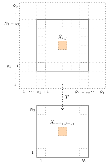
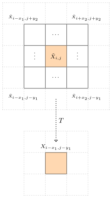
FigureΒ 1 illustrates the construction of the block-factor model: on the left (see FigΒ 1) is presented the configuration matrix defined by Eq.(2.1) and the resulted random variable after applying the transformation T𝑇T; on the right (see FigΒ 1) is exemplified how the i.i.d. model is transformed into the block-factor model .
Refer to caption
Refer to caption
Figure 1. Illustration of the block-factor type model

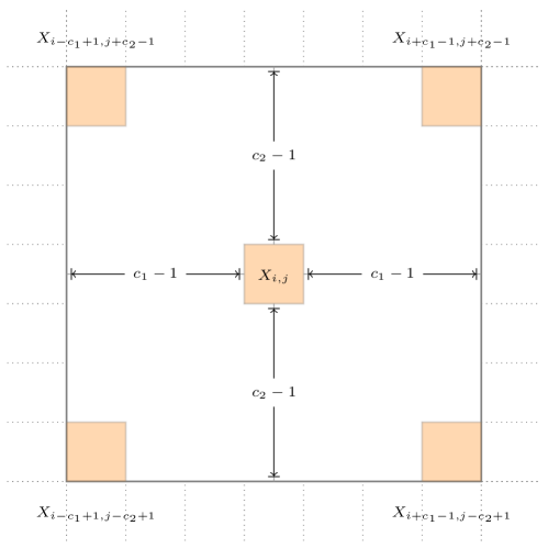
Obviously, {Xi,j| 1≀i≀N1,1≀j≀N2}conditional-setsubscript𝑋𝑖𝑗formulae-sequence1𝑖subscript𝑁11𝑗subscript𝑁2\left\{X_{i,j}\ |\ 1\leq i\leq N_{1},1\leq j\leq N_{2}\right\} forms a dependent family of random variables (see FigΒ 2).

Recall that a sequence (Wk)kβ‰₯1subscriptsubscriptπ‘Šπ‘˜π‘˜1(W_{k})_{k\geq 1} is mπ‘šm-dependent with mβ‰₯1π‘š1m\geq 1 (see Burton, Goulet and Meester [1993]), if for any hβ‰₯1β„Ž1h\geq 1 the ΟƒπœŽ\sigma-fields generated by {W1,…,Wh}subscriptπ‘Š1…subscriptπ‘Šβ„Ž\{W_{1},\dots,W_{h}\} and {Wh+m+1,…}subscriptπ‘Šβ„Žπ‘š1…\{W_{h+m+1},\dots\} are independent. From the definition of the random variables Xi,jsubscript𝑋𝑖𝑗X_{i,j} given by Eq.(2.2), we observe that for each 1≀i≀N11𝑖subscript𝑁11\leq i\leq N_{1} the sequence (Xi,j)1≀j≀N2subscriptsubscript𝑋𝑖𝑗1𝑗subscript𝑁2\left(X_{i,j}\right)_{1\leq j\leq N_{2}} is (c2βˆ’1)subscript𝑐21(c_{2}-1)-dependent and for each 1≀j≀N21𝑗subscript𝑁21\leq j\leq N_{2} the sequence (Xi,j)1≀i≀N1subscriptsubscript𝑋𝑖𝑗1𝑖subscript𝑁1\left(X_{i,j}\right)_{1\leq i\leq N_{1}} is (c1βˆ’1)subscript𝑐11(c_{1}-1)-dependent (see also FigΒ 2).

Refer to caption

Figure 2. The dependence of Xi,jsubscript𝑋𝑖𝑗X_{i,j}
Remark 2.1.

Notice that if c1=c2=1subscript𝑐1subscript𝑐21c_{1}=c_{2}=1 (x1=x2=0subscriptπ‘₯1subscriptπ‘₯20x_{1}=x_{2}=0 and y1=y2=0subscript𝑦1subscript𝑦20y_{1}=y_{2}=0) then the sequence Xi,j=X~i,jsubscript𝑋𝑖𝑗subscript~𝑋𝑖𝑗X_{i,j}=\tilde{X}_{i,j} and we are in the i.i.d. situation. In this case the distribution of the two-dimensional scan statistics can be approximated using the known methods (see Glaz, Naus and Wallenstein [2001, Chapter 16] and Glaz, Pozdnyakov and Wallenstein [2009]).

If we take N~2=1subscript~𝑁21\tilde{N}_{2}=1, which automatically implies that c2=1subscript𝑐21c_{2}=1, we obtain an one dimensional block-factor model Wi=Xi,1subscriptπ‘Šπ‘–subscript𝑋𝑖1W_{i}=X_{i,1} and the two-dimensional scan statistic becomes the usual discrete scan statistics in one dimension over a (c1βˆ’1)subscript𝑐11(c_{1}-1)-dependent sequence. The distribution of one dimensional scan statistics over this type of dependence was studied by Haiman and Preda [2013] in the particular case of Gaussian stationary 111-dependent (x1=0subscriptπ‘₯10x_{1}=0, x2=1subscriptπ‘₯21x_{2}=1 and c1=2subscript𝑐12c_{1}=2) sequences WiβˆΌπ’©β€‹(0,1)similar-tosubscriptπ‘Šπ‘–π’©01W_{i}\sim{\mathcal{N}}(0,1) of random variables generated by a two block-factor of the form

Wi=a​Ui+b​Ui+1,iβ‰₯1,formulae-sequencesubscriptπ‘Šπ‘–π‘Žsubscriptπ‘ˆπ‘–π‘subscriptπ‘ˆπ‘–1𝑖1W_{i}=aU_{i}+bU_{i+1},\ \ i\geq 1,

where a2+b2=1superscriptπ‘Ž2superscript𝑏21a^{2}+b^{2}=1 and (Ui)iβ‰₯1subscriptsubscriptπ‘ˆπ‘–π‘–1\left(U_{i}\right)_{i\geq 1} is an i.i.d. sequence of 𝒩​(0,1)𝒩01{\mathcal{N}}(0,1) random variables.

An application of the one dimensional scan statistics over a sequence of moving average of order qπ‘žq (c1=q+1subscript𝑐1π‘ž1c_{1}=q+1) is presented in SectionΒ 4.2.

Based on the model presented in this section, in SectionΒ 3 we give an approximation for the distribution of two-dimensional scan statistic over the random field generated by the family Xi,jsubscript𝑋𝑖𝑗X_{i,j} and the corresponding error bounds.

3. Approximation and error bounds

In this section we present the methodology used to obtain the approximation of the two-dimensional discrete scan statistics distribution over the field generated by the block-factor model described in SectionΒ 2. Let’s consider the scanning window of size m1Γ—m2subscriptπ‘š1subscriptπ‘š2m_{1}\times m_{2} with m1β‰₯2subscriptπ‘š12m_{1}\geq 2, m2β‰₯2subscriptπ‘š22m_{2}\geq 2 and assume that for s∈{1,2}𝑠12s\in\{1,2\}, N~s=(Ls+1)​(ms+csβˆ’2)subscript~𝑁𝑠subscript𝐿𝑠1subscriptπ‘šπ‘ subscript𝑐𝑠2\tilde{N}_{s}=(L_{s}+1)(m_{s}+c_{s}-2) where L1subscript𝐿1L_{1}, L2subscript𝐿2L_{2} are positive integers. Observe that

Ns=Ls​(ms+csβˆ’2)+msβˆ’1,s∈{1,2}formulae-sequencesubscript𝑁𝑠subscript𝐿𝑠subscriptπ‘šπ‘ subscript𝑐𝑠2subscriptπ‘šπ‘ 1𝑠12N_{s}=L_{s}(m_{s}+c_{s}-2)+m_{s}-1,\,s\in\{1,2\}

and define the sequence

Zk=max1≀i1≀L1​(m1+c1βˆ’2)(kβˆ’1)​(m2+c2βˆ’2)+1≀i2≀k​(m2+c2βˆ’2)⁑Yi1,i2,k∈{1,2,…,L2}.formulae-sequencesubscriptπ‘π‘˜subscript1subscript𝑖1subscript𝐿1subscriptπ‘š1subscript𝑐12π‘˜1subscriptπ‘š2subscript𝑐221subscript𝑖2π‘˜subscriptπ‘š2subscript𝑐22subscriptπ‘Œsubscript𝑖1subscript𝑖2π‘˜12…subscript𝐿2Z_{k}=\max_{\begin{subarray}{c}1\leq i_{1}\leq L_{1}(m_{1}+c_{1}-2)\\ (k-1)(m_{2}+c_{2}-2)+1\leq i_{2}\leq k(m_{2}+c_{2}-2)\end{subarray}}{Y_{i_{1},i_{2}}},\,\,\,\,k\in\{1,2,\dots,L_{2}\}. (3.1)

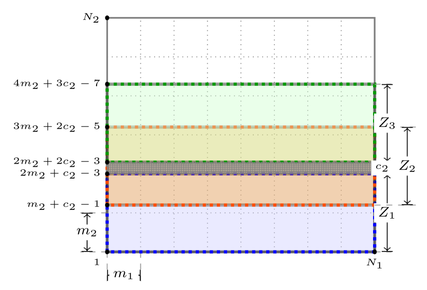
The random variables Zksubscriptπ‘π‘˜Z_{k} represent the scan statistics on the overlapping N1Γ—2​(m2+c2βˆ’2)βˆ’(c2βˆ’1)subscript𝑁12subscriptπ‘š2subscript𝑐22subscript𝑐21N_{1}\times 2(m_{2}+c_{2}-2)-(c_{2}-1) rectangular regions

β„›k=[1,N1]Γ—[(kβˆ’1)​(m2+c2βˆ’2)+1,(k+1)​(m2+c2βˆ’2)βˆ’(c2βˆ’1)].subscriptβ„›π‘˜1subscript𝑁1π‘˜1subscriptπ‘š2subscript𝑐221π‘˜1subscriptπ‘š2subscript𝑐22subscript𝑐21{\mathcal{R}}_{k}=[1,N_{1}]\times[(k-1)(m_{2}+c_{2}-2)+1,(k+1)(m_{2}+c_{2}-2)-(c_{2}-1)].

Refer to caption

Figure 3. Illustration of Zksubscriptπ‘π‘˜Z_{k} emphasizing the 111-dependence
Remark 3.1.

If we consider the extreme situation when c2=m2=1subscript𝑐2subscriptπ‘š21c_{2}=m_{2}=1 (or c1=m1=1subscript𝑐1subscriptπ‘š11c_{1}=m_{1}=1), that is when we have row (column) independence and we are scanning only on rows (columns), then the sequence described by Eq.(3.1) is no longer well defined. In this case we define

Zk=max1≀i1≀L1​(m1+c1βˆ’2)⁑Yi1,k,k∈{1,2,…,L2},formulae-sequencesubscriptπ‘π‘˜subscript1subscript𝑖1subscript𝐿1subscriptπ‘š1subscript𝑐12subscriptπ‘Œsubscript𝑖1π‘˜π‘˜12…subscript𝐿2Z_{k}=\max_{1\leq i_{1}\leq L_{1}(m_{1}+c_{1}-2)}{Y_{i_{1},k}},\,\,\,\,k\in\{1,2,\dots,L_{2}\}, (3.2)

where Yi1,k=βˆ‘i=i1i1+m1βˆ’1Xi,k.subscriptπ‘Œsubscript𝑖1π‘˜superscriptsubscript𝑖subscript𝑖1subscript𝑖1subscriptπ‘š11subscriptπ‘‹π‘–π‘˜Y_{i_{1},k}=\sum_{i=i_{1}}^{i_{1}+m_{1}-1}{X_{i,k}}.

We observe that from Eq.(3.1) the set of random variables {Z1,…,ZL2}subscript𝑍1…subscript𝑍subscript𝐿2\{Z_{1},\dots,Z_{L_{2}}\} is 1-dependent (see also FigureΒ 3). Indeed, we have

Zkβˆ’1subscriptπ‘π‘˜1\displaystyle Z_{k-1} βˆˆΟƒβ€‹{Xi,j|1≀i≀N1,(kβˆ’2)​(m2+c2βˆ’2)+1≀j≀k​(m2+c2βˆ’2)βˆ’(c2βˆ’1)}absent𝜎conditional-setsubscript𝑋𝑖𝑗formulae-sequence1𝑖subscript𝑁1π‘˜2subscriptπ‘š2subscript𝑐221π‘—π‘˜subscriptπ‘š2subscript𝑐22subscript𝑐21\displaystyle\in\sigma\left\{X_{i,j}|1\leq i\leq N_{1},(k-2)(m_{2}+c_{2}-2)+1\leq j\leq k(m_{2}+c_{2}-2)-(c_{2}-1)\right\}
βˆˆΟƒβ€‹{X~i,j|1≀i≀N~1,(kβˆ’2)​(m2+cβˆ’2βˆ’2)+1≀j≀k​(m2+c2βˆ’2)}absent𝜎conditional-setsubscript~𝑋𝑖𝑗formulae-sequence1𝑖subscript~𝑁1π‘˜2subscriptπ‘š2𝑐221π‘—π‘˜subscriptπ‘š2subscript𝑐22\displaystyle\in\sigma\left\{\tilde{X}_{i,j}|1\leq i\leq\tilde{N}_{1},(k-2)(m_{2}+c-2-2)+1\leq j\leq k(m_{2}+c_{2}-2)\right\}

and similarly,

Zksubscriptπ‘π‘˜\displaystyle Z_{k} βˆˆΟƒβ€‹{X~i,j|1≀i≀N~1,(kβˆ’1)​(m2+c2βˆ’2)+1≀j≀(k+1)​(m2+c2βˆ’2)},absent𝜎conditional-setsubscript~𝑋𝑖𝑗formulae-sequence1𝑖subscript~𝑁1π‘˜1subscriptπ‘š2subscript𝑐221π‘—π‘˜1subscriptπ‘š2subscript𝑐22\displaystyle\in\sigma\left\{\tilde{X}_{i,j}|1\leq i\leq\tilde{N}_{1},(k-1)(m_{2}+c_{2}-2)+1\leq j\leq(k+1)(m_{2}+c_{2}-2)\right\},
Zk+1subscriptπ‘π‘˜1\displaystyle Z_{k+1} βˆˆΟƒβ€‹{X~i,j|1≀i≀N~1,k​(m2+c2βˆ’2)+1≀j≀(k+2)​(m2+c2βˆ’2)}.absent𝜎conditional-setsubscript~𝑋𝑖𝑗formulae-sequence1𝑖subscript~𝑁1π‘˜subscriptπ‘š2subscript𝑐221π‘—π‘˜2subscriptπ‘š2subscript𝑐22\displaystyle\in\sigma\left\{\tilde{X}_{i,j}|1\leq i\leq\tilde{N}_{1},k(m_{2}+c_{2}-2)+1\leq j\leq(k+2)(m_{2}+c_{2}-2)\right\}.

From the above relations, the measurability of T𝑇T from the definition of the dependent model {Xi,j|1≀i≀N1,1≀j≀N2}conditional-setsubscript𝑋𝑖𝑗formulae-sequence1𝑖subscript𝑁11𝑗subscript𝑁2\left\{X_{i,j}|1\leq i\leq N_{1},1\leq j\leq N_{2}\right\} and the independence of the sequence {X~i,j|1≀i≀N~1,1≀j≀N~2}conditional-setsubscript~𝑋𝑖𝑗formulae-sequence1𝑖subscript~𝑁11𝑗subscript~𝑁2\left\{\tilde{X}_{i,j}|1\leq i\leq\tilde{N}_{1},1\leq j\leq\tilde{N}_{2}\right\} we conclude that the sequence (Zk)1≀k≀L2subscriptsubscriptπ‘π‘˜1π‘˜subscript𝐿2\left(Z_{k}\right)_{1\leq k\leq L_{2}} is 1-dependent. Since X~i,jsubscript~𝑋𝑖𝑗\tilde{X}_{i,j} are identically distributed we deduce stationarity of the random variables Zksubscriptπ‘π‘˜Z_{k}.

Notice that from Eq.(3.1) and the definition of the two-dimensional scan statistics in Eq.(2.1) we have the following relation

S=max1≀k≀L2⁑Zk.𝑆subscript1π‘˜subscript𝐿2subscriptπ‘π‘˜S=\max_{1\leq k\leq L_{2}}Z_{k}. (3.3)

The relation described by Eq.(3.3) is the key idea behind our approximation, i.e. the scan statistic random variable can be expressed as a maximum of 1-dependent stationary sequence of random variables. The approximation methodology that we use is based on the following result developed in Haiman [1999, Theorem 4] and improved in Amărioarei [2012, Theorem 2.6]:
Let (Wk)kβ‰₯1subscriptsubscriptπ‘Šπ‘˜π‘˜1(W_{k})_{k\geq 1} be a stationary 1-dependent sequence of random variables and for x<sup{u|ℙ​(W1≀u)<1}π‘₯supremumconditional-set𝑒ℙsubscriptπ‘Š1𝑒1x<\sup\{u|{\mathbb{P}}(W_{1}\leq u)<1\}, consider

qm=qm​(x)=ℙ​(max⁑(W1,…,Wm)≀x).subscriptπ‘žπ‘šsubscriptπ‘žπ‘šπ‘₯β„™subscriptπ‘Š1…subscriptπ‘Šπ‘šπ‘₯q_{m}=q_{m}(x)={\mathbb{P}}(\max(W_{1},\dots,W_{m})\leq x). (3.4)
Theorem 3.2.

Assume that xπ‘₯x is such that q1​(x)β‰₯1βˆ’Ξ±β‰₯0.9subscriptπ‘ž1π‘₯1𝛼0.9q_{1}(x)\geq 1-{\alpha}\geq 0.9 and define Ξ·=1+lβ€‹Ξ±πœ‚1𝑙𝛼\eta=1+l{\alpha} with l=l​(Ξ±)>t23​(Ξ±)𝑙𝑙𝛼superscriptsubscript𝑑23𝛼l=l({\alpha})>t_{2}^{3}({\alpha}) and t2​(Ξ±)subscript𝑑2𝛼t_{2}({\alpha}) the second root in magnitude of the equation α​t3βˆ’t+1=0𝛼superscript𝑑3𝑑10{\alpha}t^{3}-t+1=0. Then the following relation holds

|qmβˆ’2​q1βˆ’q2[1+q1βˆ’q2+2​(q1βˆ’q2)2]m|≀m​F​(Ξ±,m)​(1βˆ’q1)2,subscriptπ‘žπ‘š2subscriptπ‘ž1subscriptπ‘ž2superscriptdelimited-[]1subscriptπ‘ž1subscriptπ‘ž22superscriptsubscriptπ‘ž1subscriptπ‘ž22π‘šπ‘šπΉπ›Όπ‘šsuperscript1subscriptπ‘ž12\left|q_{m}-\frac{2q_{1}-q_{2}}{\left[1+q_{1}-q_{2}+2(q_{1}-q_{2})^{2}\right]^{m}}\right|\leq mF({\alpha},m)(1-q_{1})^{2}, (3.5)

with

F​(Ξ±,m)=1+3m+[Γ​(Ξ±)m+K​(Ξ±)]​(1βˆ’q1),πΉπ›Όπ‘š13π‘šdelimited-[]Ξ“π›Όπ‘šπΎπ›Ό1subscriptπ‘ž1F({\alpha},m)=1+\frac{3}{m}+\left[\frac{{\Gamma}({\alpha})}{m}+K({\alpha})\right](1-q_{1}), (3.6)

and where Γ​(Ξ±)=L​(Ξ±)+E​(Ξ±)Γ𝛼𝐿𝛼𝐸𝛼{\Gamma}({\alpha})=L({\alpha})+E({\alpha}) and

K​(Ξ±)𝐾𝛼\displaystyle K({\alpha}) =11βˆ’3​α(1βˆ’Ξ±)2+2​l​(1+3​α)​2+3​lβ€‹Ξ±βˆ’Ξ±β€‹(2βˆ’l​α)​(1+l​α)2[1βˆ’Ξ±β€‹(1+l​α)2]31βˆ’2​α​(1+l​α)[1βˆ’Ξ±β€‹(1+l​α)2]2,absent113𝛼superscript1𝛼22𝑙13𝛼23𝑙𝛼𝛼2𝑙𝛼superscript1𝑙𝛼2superscriptdelimited-[]1𝛼superscript1𝑙𝛼2312𝛼1𝑙𝛼superscriptdelimited-[]1𝛼superscript1𝑙𝛼22\displaystyle=\frac{\frac{11-3{\alpha}}{(1-{\alpha})^{2}}+2l(1+3{\alpha})\frac{2+3l{\alpha}-{\alpha}(2-l{\alpha})(1+l{\alpha})^{2}}{\left[1-{\alpha}(1+l{\alpha})^{2}\right]^{3}}}{1-\frac{2{\alpha}(1+l{\alpha})}{\left[1-{\alpha}(1+l{\alpha})^{2}\right]^{2}}}, (3.7)
L​(Ξ±)𝐿𝛼\displaystyle L({\alpha}) =3​K​(Ξ±)​(1+Ξ±+3​α2)​[1+Ξ±+3​α2+K​(Ξ±)​α3]+Ξ±6​K3​(Ξ±),absent3𝐾𝛼1𝛼3superscript𝛼2delimited-[]1𝛼3superscript𝛼2𝐾𝛼superscript𝛼3superscript𝛼6superscript𝐾3𝛼\displaystyle=3K({\alpha})(1+{\alpha}+3{\alpha}^{2})[1+{\alpha}+3{\alpha}^{2}+K({\alpha}){\alpha}^{3}]+{\alpha}^{6}K^{3}({\alpha}),
+9​α​(4+3​α+3​α2)+55.19𝛼43𝛼3superscript𝛼255.1\displaystyle+9{\alpha}(4+3{\alpha}+3{\alpha}^{2})+55.1 (3.8)
E​(Ξ±)𝐸𝛼\displaystyle E({\alpha}) =Ξ·5​[1+(1βˆ’2​α)​η]4​[1+α​(Ξ·βˆ’2)]​[1+Ξ·+(1βˆ’3​α)​η2]2​(1βˆ’Ξ±β€‹Ξ·2)4​[(1βˆ’Ξ±β€‹Ξ·2)2βˆ’Ξ±β€‹Ξ·2​(1+Ξ·βˆ’2​α​η)2].absentsuperscriptπœ‚5superscriptdelimited-[]112π›Όπœ‚4delimited-[]1π›Όπœ‚2delimited-[]1πœ‚13𝛼superscriptπœ‚22superscript1𝛼superscriptπœ‚24delimited-[]superscript1𝛼superscriptπœ‚22𝛼superscriptπœ‚2superscript1πœ‚2π›Όπœ‚2\displaystyle=\frac{\eta^{5}\left[1+(1-2{\alpha})\eta\right]^{4}\left[1+{\alpha}(\eta-2)\right]\left[1+\eta+(1-3{\alpha})\eta^{2}\right]}{2(1-{\alpha}\eta^{2})^{4}\left[(1-{\alpha}\eta^{2})^{2}-{\alpha}\eta^{2}(1+\eta-2{\alpha}\eta)^{2}\right]}. (3.9)

Following the approach in AmΔƒrioarei and Preda [2013] for three dimensional scan statistics, we obtain an approximation formula for the distribution of two-dimensional scan statistic S𝑆S along with the corresponding error bounds, in two steps as follows.

Define for r∈{2,3}π‘Ÿ23r\in\{2,3\},

Qr=Qr​(n)=ℙ​(β‹‚k=1rβˆ’1{Zk≀n})=ℙ​(max1≀i1≀L1​(m1+c1βˆ’2)1≀i2≀(rβˆ’1)​(m2+c2βˆ’2)⁑Yi1,i2≀n).subscriptπ‘„π‘Ÿsubscriptπ‘„π‘Ÿπ‘›β„™superscriptsubscriptπ‘˜1π‘Ÿ1subscriptπ‘π‘˜π‘›β„™subscript1subscript𝑖1subscript𝐿1subscriptπ‘š1subscript𝑐121subscript𝑖2π‘Ÿ1subscriptπ‘š2subscript𝑐22subscriptπ‘Œsubscript𝑖1subscript𝑖2𝑛Q_{r}=Q_{r}(n)=\displaystyle{\mathbb{P}}\left(\bigcap_{k=1}^{r-1}\{Z_{k}\leq n\}\right)=\displaystyle{\mathbb{P}}\left(\max_{\begin{subarray}{c}1\leq i_{1}\leq L_{1}(m_{1}+c_{1}-2)\\ 1\leq i_{2}\leq(r-1)(m_{2}+c_{2}-2)\end{subarray}}{Y_{i_{1},i_{2}}}\leq n\right). (3.10)

For n𝑛n such that Q2​(n)β‰₯1βˆ’Ξ±1β‰₯0.9subscript𝑄2𝑛1subscript𝛼10.9Q_{2}(n)\geq 1-{\alpha}_{1}\geq 0.9, we apply the result in TheoremΒ 3.2 to obtain the first step approximation

|ℙ​(S≀n)βˆ’2​Q2βˆ’Q3[1+Q2βˆ’Q3+2​(Q2βˆ’Q3)2]L2|≀L2​F​(Ξ±1,L2)​(1βˆ’Q2)2.ℙ𝑆𝑛2subscript𝑄2subscript𝑄3superscriptdelimited-[]1subscript𝑄2subscript𝑄32superscriptsubscript𝑄2subscript𝑄32subscript𝐿2subscript𝐿2𝐹subscript𝛼1subscript𝐿2superscript1subscript𝑄22\left|{\mathbb{P}}\left(S\leq n\right)-\frac{2Q_{2}-Q_{3}}{\left[1+Q_{2}-Q_{3}+2(Q_{2}-Q_{3})^{2}\right]^{L_{2}}}\right|\leq L_{2}F({\alpha}_{1},L_{2})(1-Q_{2})^{2}. (3.11)

In order to evaluate the approximation in Eq.(3.11) one has to find approximations for the quantities Q2subscript𝑄2Q_{2} and Q3subscript𝑄3Q_{3}. To achieve this, we apply again the result of TheoremΒ 3.2. We define, as in Eq.(3.1), for each r∈{2,3}π‘Ÿ23r\in\{2,3\} and l∈{1,2,…,L1}𝑙12…subscript𝐿1l\in\{1,2,\dots,L_{1}\} the random variables

Zl(r)=max(lβˆ’1)​(m1+c1βˆ’2)+1≀i1≀l​(m1+c1βˆ’2)1≀i2≀(rβˆ’1)​(m2+c2βˆ’2)⁑Yi1,i2.subscriptsuperscriptπ‘π‘Ÿπ‘™subscript𝑙1subscriptπ‘š1subscript𝑐121subscript𝑖1𝑙subscriptπ‘š1subscript𝑐121subscript𝑖2π‘Ÿ1subscriptπ‘š2subscript𝑐22subscriptπ‘Œsubscript𝑖1subscript𝑖2Z^{(r)}_{l}=\max_{\begin{subarray}{c}(l-1)(m_{1}+c_{1}-2)+1\leq i_{1}\leq l(m_{1}+c_{1}-2)\\ 1\leq i_{2}\leq(r-1)(m_{2}+c_{2}-2)\end{subarray}}{Y_{i_{1},i_{2}}}. (3.12)

As described in the case of the sequence Zksubscriptπ‘π‘˜Z_{k}, we deduce that the random variables Zl(r)subscriptsuperscriptπ‘π‘Ÿπ‘™Z^{(r)}_{l} defined by Eq.(3.12) are stationary, 111-dependent and the following relation holds:

Qr=ℙ​(max1≀l≀L1⁑Zl(r)≀n),r∈{2,3}.formulae-sequencesubscriptπ‘„π‘Ÿβ„™subscript1𝑙subscript𝐿1subscriptsuperscriptπ‘π‘Ÿπ‘™π‘›π‘Ÿ23Q_{r}={\mathbb{P}}\left(\max_{1\leq l\leq L_{1}}Z^{(r)}_{l}\leq n\right),\ \ \ r\in\{2,3\}. (3.13)

Denoting, for u,v∈{2,3}𝑒𝑣23u,v\in\{2,3\}

Qu​v=Qu​v​(n)=ℙ​(β‹‚l=1uβˆ’1{Zl(v)≀n})=ℙ​(max1≀i1≀(uβˆ’1)​(m1+c1βˆ’2)1≀i2≀(vβˆ’1)​(m2+c2βˆ’2)⁑Yi1,i2≀n)subscript𝑄𝑒𝑣subscript𝑄𝑒𝑣𝑛ℙsuperscriptsubscript𝑙1𝑒1subscriptsuperscript𝑍𝑣𝑙𝑛ℙsubscript1subscript𝑖1𝑒1subscriptπ‘š1subscript𝑐121subscript𝑖2𝑣1subscriptπ‘š2subscript𝑐22subscriptπ‘Œsubscript𝑖1subscript𝑖2𝑛Q_{uv}=Q_{uv}(n)=\displaystyle{\mathbb{P}}\left(\bigcap_{l=1}^{u-1}\{Z^{(v)}_{l}\leq n\}\right)=\displaystyle{\mathbb{P}}\left(\max_{\begin{subarray}{c}1\leq i_{1}\leq(u-1)(m_{1}+c_{1}-2)\\ 1\leq i_{2}\leq(v-1)(m_{2}+c_{2}-2)\end{subarray}}{Y_{i_{1},i_{2}}}\leq n\right) (3.14)

then, under the supplementary condition that n𝑛n is such that Q23​(n)β‰₯1βˆ’Ξ±2β‰₯0.9subscript𝑄23𝑛1subscript𝛼20.9Q_{23}(n)\geq 1-{\alpha}_{2}\geq 0.9, we apply TheoremΒ 3.2 to obtain

|Qrβˆ’2​Q2​rβˆ’Q3​r[1+Q2​rβˆ’Q3​r+2​(Q2​rβˆ’Q3​r)2]L1|≀L1​F​(Ξ±2,L1)​(1βˆ’Q2​r)2.subscriptπ‘„π‘Ÿ2subscript𝑄2π‘Ÿsubscript𝑄3π‘Ÿsuperscriptdelimited-[]1subscript𝑄2π‘Ÿsubscript𝑄3π‘Ÿ2superscriptsubscript𝑄2π‘Ÿsubscript𝑄3π‘Ÿ2subscript𝐿1subscript𝐿1𝐹subscript𝛼2subscript𝐿1superscript1subscript𝑄2π‘Ÿ2\left|Q_{r}-\frac{2Q_{2r}-Q_{3r}}{\left[1+Q_{2r}-Q_{3r}+2(Q_{2r}-Q_{3r})^{2}\right]^{L_{1}}}\right|\leq L_{1}F({\alpha}_{2},L_{1})(1-Q_{2r})^{2}. (3.15)

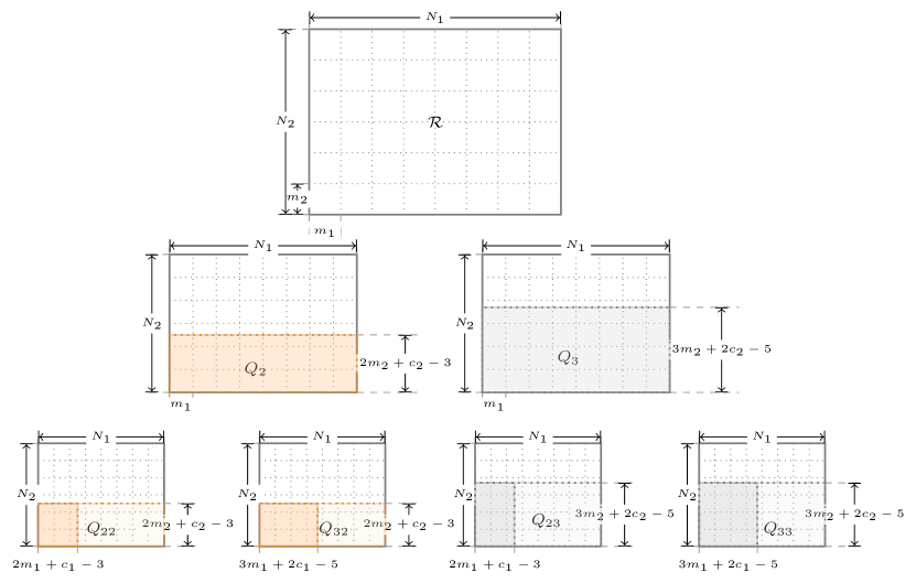
Combining Eq.(3.11) and Eq.(3.15) we find an approximation formula for the distribution of the two-dimensional scan statistic depending on the values of Q22subscript𝑄22Q_{22}, Q23subscript𝑄23Q_{23}, Q32subscript𝑄32Q_{32} and Q33subscript𝑄33Q_{33}. There are no exact formulas for Qu​vsubscript𝑄𝑒𝑣Q_{uv}, u,v∈{2,3}𝑒𝑣23u,v\in\{2,3\}, thus these quantities will be evaluated using Monte Carlo simulation. The approximation process is summarized by the diagram in FigureΒ 4:

Refer to caption

Figure 4. Illustration of the approximation process
Remark 3.3.

If N~1subscript~𝑁1\tilde{N}_{1} and N~2subscript~𝑁2\tilde{N}_{2} are not multiples of m1+c1βˆ’2subscriptπ‘š1subscript𝑐12m_{1}+c_{1}-2 and m2+c2βˆ’2subscriptπ‘š2subscript𝑐22m_{2}+c_{2}-2, respectively, then we take Lj+1=⌊N~jmj+cjβˆ’2βŒ‹subscript𝐿𝑗1subscript~𝑁𝑗subscriptπ‘šπ‘—subscript𝑐𝑗2L_{j}+1=\left\lfloor{\frac{\tilde{N}_{j}}{m_{j}+c_{j}-2}}\right\rfloor for j∈{1,2}𝑗12j\in\{1,2\}. Based on the inequalities

ℙ​(Sm1,m2​(M1,M2)≀n)≀ℙ​(Sm1,m2​(N1,N2)≀n)≀ℙ​(Sm1,m2​(T1,T2)≀n),β„™subscript𝑆subscriptπ‘š1subscriptπ‘š2subscript𝑀1subscript𝑀2𝑛ℙsubscript𝑆subscriptπ‘š1subscriptπ‘š2subscript𝑁1subscript𝑁2𝑛ℙsubscript𝑆subscriptπ‘š1subscriptπ‘š2subscript𝑇1subscript𝑇2𝑛{\mathbb{P}}\left(S_{m_{1},m_{2}}(M_{1},M_{2})\leq n\right)\leq{\mathbb{P}}\left(S_{m_{1},m_{2}}(N_{1},N_{2})\leq n\right)\leq{\mathbb{P}}\left(S_{m_{1},m_{2}}(T_{1},T_{2})\leq n\right), (3.16)

where for j∈{1,2}𝑗12j\in\{1,2\} we consider Mj=(Lj+2)​(mj+cjβˆ’2)βˆ’(cjβˆ’1)subscript𝑀𝑗subscript𝐿𝑗2subscriptπ‘šπ‘—subscript𝑐𝑗2subscript𝑐𝑗1M_{j}=(L_{j}+2)(m_{j}+c_{j}-2)-(c_{j}-1) and Tj=(Lj+1)​(mj+cjβˆ’2)βˆ’(cjβˆ’1)subscript𝑇𝑗subscript𝐿𝑗1subscriptπ‘šπ‘—subscript𝑐𝑗2subscript𝑐𝑗1T_{j}=(L_{j}+1)(m_{j}+c_{j}-2)-(c_{j}-1), we can approximate the distribution of the scan statistics by linear interpolation.

3.1. Computing the error bounds

For the error computation we have to notice that there are three expressions involved: the first one is the theoretical error (Ea​p​psubscriptπΈπ‘Žπ‘π‘E_{app}) obtained from the substitution of Eq.(3.15) in Eq.(3.11) whereas the other two are simulations errors, one corresponding to the approximation formula (Es​fsubscript𝐸𝑠𝑓E_{sf}) and the other to the error formula (Es​a​p​psubscriptπΈπ‘ π‘Žπ‘π‘E_{sapp}). In what follows we will deal with each of them separately. To simplify the presentation it will be convenient to introduce the following notations:

H​(x,y,m)𝐻π‘₯π‘¦π‘š\displaystyle H(x,y,m) =2​xβˆ’y[1+xβˆ’y+2​(xβˆ’y)2]m,Ξ±1=1βˆ’Q3,Ξ±2=1βˆ’Q23,formulae-sequenceabsent2π‘₯𝑦superscriptdelimited-[]1π‘₯𝑦2superscriptπ‘₯𝑦2π‘šformulae-sequencesubscript𝛼11subscript𝑄3subscript𝛼21subscript𝑄23\displaystyle=\frac{2x-y}{[1+x-y+2(x-y)^{2}]^{m}},\ {\alpha}_{1}=1-Q_{3},\ {\alpha}_{2}=1-Q_{23},
F1subscript𝐹1\displaystyle F_{1} =F​(Ξ±2,L1),F2=F​(Ξ±1,L2),Rs=H​(Q2​s,Q3​s,L1),s∈{2,3}.formulae-sequenceabsent𝐹subscript𝛼2subscript𝐿1formulae-sequencesubscript𝐹2𝐹subscript𝛼1subscript𝐿2formulae-sequencesubscript𝑅𝑠𝐻subscript𝑄2𝑠subscript𝑄3𝑠subscript𝐿1𝑠23\displaystyle=F({\alpha}_{2},L_{1}),\ F_{2}=F({\alpha}_{1},L_{2}),\ R_{s}=H\left(Q_{2s},Q_{3s},L_{1}\right),\ s\in\{2,3\}.

Notice that the choice for the thresholds Ξ±1subscript𝛼1{\alpha}_{1} and Ξ±2subscript𝛼2{\alpha}_{2} is natural since we have the inequalities Q3≀Q2subscript𝑄3subscript𝑄2Q_{3}\leq Q_{2} and Q23≀Q22subscript𝑄23subscript𝑄22Q_{23}\leq Q_{22}. Based on mean value theorem in two dimensions, one can easily verify that if yi≀xisubscript𝑦𝑖subscriptπ‘₯𝑖y_{i}\leq x_{i}, i∈{1,2}𝑖12i\in\{1,2\} then we have the relation

|H​(x1,y1,m)βˆ’H​(x2,y2,m)|≀m​[|x1βˆ’x2|+|y1βˆ’y2|].𝐻subscriptπ‘₯1subscript𝑦1π‘šπ»subscriptπ‘₯2subscript𝑦2π‘šπ‘šdelimited-[]subscriptπ‘₯1subscriptπ‘₯2subscript𝑦1subscript𝑦2\left|H(x_{1},y_{1},m)-H(x_{2},y_{2},m)\right|\leq m\left[|x_{1}-x_{2}|+|y_{1}-y_{2}|\right]. (3.17)

Rewriting Eq.(3.11) using the above notations and applying the inequality in Eq.(3.17) we can write

|ℙ​(S≀n)βˆ’H​(R2,R3,L2)|ℙ𝑆𝑛𝐻subscript𝑅2subscript𝑅3subscript𝐿2\displaystyle\left|{\mathbb{P}}(S\leq n)-H\left(R_{2},R_{3},L_{2}\right)\right| ≀|ℙ​(S≀n)βˆ’H​(Q2,Q3,L2)|+absentlimit-fromℙ𝑆𝑛𝐻subscript𝑄2subscript𝑄3subscript𝐿2\displaystyle\leq\left|{\mathbb{P}}(S\leq n)-H\left(Q_{2},Q_{3},L_{2}\right)\right|+
|H​(Q2,Q3,L2)βˆ’H​(R2,R3,L2)|𝐻subscript𝑄2subscript𝑄3subscript𝐿2𝐻subscript𝑅2subscript𝑅3subscript𝐿2\displaystyle\left|H\left(Q_{2},Q_{3},L_{2}\right)-H\left(R_{2},R_{3},L_{2}\right)\right|
≀L2​F2​(1βˆ’Q2)2+L2​[|Q2βˆ’R2|+|Q3βˆ’R3|].absentsubscript𝐿2subscript𝐹2superscript1subscript𝑄22subscript𝐿2delimited-[]subscript𝑄2subscript𝑅2subscript𝑄3subscript𝑅3\displaystyle\leq L_{2}F_{2}\left(1-Q_{2}\right)^{2}+L_{2}\left[|Q_{2}-R_{2}|+|Q_{3}-R_{3}|\right]. (3.18)

If we substitute Eq.(3.15) in Eq.(3.18) and take B2=1βˆ’R2+L1​F1​(1βˆ’Q22)2subscript𝐡21subscript𝑅2subscript𝐿1subscript𝐹1superscript1subscript𝑄222B_{2}=1-R_{2}+L_{1}F_{1}(1-Q_{22})^{2}, then the theoretical approximation error is given by

Ea​p​p=L2​F2​B22+L1​L2​F1​[(1βˆ’Q22)2+(1βˆ’Q23)2].subscriptπΈπ‘Žπ‘π‘subscript𝐿2subscript𝐹2superscriptsubscript𝐡22subscript𝐿1subscript𝐿2subscript𝐹1delimited-[]superscript1subscript𝑄222superscript1subscript𝑄232E_{app}=L_{2}F_{2}B_{2}^{2}+L_{1}L_{2}F_{1}\left[(1-Q_{22})^{2}+(1-Q_{23})^{2}\right]. (3.19)

To compute the simulation error corresponding to the approximation formula let us denote with Q^u​vsubscript^𝑄𝑒𝑣\hat{Q}_{uv} the simulated values corresponding to Qu​vsubscript𝑄𝑒𝑣Q_{uv} for each u,v∈{2,3}𝑒𝑣23u,v\in\{2,3\}. Usually between the true and the estimated values we have a relation of the type

|Qu​vβˆ’Q^u​v|≀βu​v.subscript𝑄𝑒𝑣subscript^𝑄𝑒𝑣subscript𝛽𝑒𝑣\left|Q_{uv}-\hat{Q}_{uv}\right|\leq\beta_{uv}. (3.20)

Indeed, if I​T​E​R𝐼𝑇𝐸𝑅ITER is the number of iterations used in the Monte Carlo simulation algorithm for the estimation of Qu​vsubscript𝑄𝑒𝑣Q_{uv} then, one can consider, for example, the bound Ξ²u​v=1.96​Q^u​v​(1βˆ’Q^u​v)I​T​E​Rsubscript𝛽𝑒𝑣1.96subscript^𝑄𝑒𝑣1subscript^𝑄𝑒𝑣𝐼𝑇𝐸𝑅\beta_{uv}=1.96\sqrt{\frac{\hat{Q}_{uv}(1-\hat{Q}_{uv})}{ITER}} with a 95%percent9595\% confidence level. Taking for r∈{2,3}π‘Ÿ23r\in\{2,3\}, Q^r=H​(Q^2​r,Q^3​r,L1)subscript^π‘„π‘Ÿπ»subscript^𝑄2π‘Ÿsubscript^𝑄3π‘Ÿsubscript𝐿1\hat{Q}_{r}=H\left(\hat{Q}_{2r},\hat{Q}_{3r},L_{1}\right) to be the simulated values that corresponds to Qrsubscriptπ‘„π‘ŸQ_{r} and applying Eq.(3.17) whenever Q^3≀Q^2subscript^𝑄3subscript^𝑄2\hat{Q}_{3}\leq\hat{Q}_{2} we get

|H​(R2,R3,L2)βˆ’H​(Q^2,Q^3,L2)|𝐻subscript𝑅2subscript𝑅3subscript𝐿2𝐻subscript^𝑄2subscript^𝑄3subscript𝐿2\displaystyle\left|H\left(R_{2},R_{3},L_{2}\right)-H\left(\hat{Q}_{2},\hat{Q}_{3},L_{2}\right)\right| ≀L2​[|R2βˆ’Q^2|+|R3βˆ’Q^3|]absentsubscript𝐿2delimited-[]subscript𝑅2subscript^𝑄2subscript𝑅3subscript^𝑄3\displaystyle\leq L_{2}\left[\left|R_{2}-\hat{Q}_{2}\right|+\left|R_{3}-\hat{Q}_{3}\right|\right]
≀L1L2[|Q22βˆ’Q^22|+|Q23βˆ’Q^23|+\displaystyle\leq L_{1}L_{2}\left[\left|Q_{22}-\hat{Q}_{22}\right|+\left|Q_{23}-\hat{Q}_{23}\right|+\right.
|Q32βˆ’Q^32|+|Q33βˆ’Q^33|].\displaystyle\left.\left|Q_{32}-\hat{Q}_{32}\right|+\left|Q_{33}-\hat{Q}_{33}\right|\right]. (3.21)

Combining Eq.(3.21) and Eq.(3.20) we obtain the simulation error associated with the approximation formula

Es​f=L1​L2​(Ξ²22+Ξ²23+Ξ²32+Ξ²33).subscript𝐸𝑠𝑓subscript𝐿1subscript𝐿2subscript𝛽22subscript𝛽23subscript𝛽32subscript𝛽33E_{sf}=L_{1}L_{2}(\beta_{22}+\beta_{23}+\beta_{32}+\beta_{33}). (3.22)

Finally, introducing

C2​vsubscript𝐢2𝑣\displaystyle C_{2v} =1βˆ’Q^2​v+Ξ²2​v,v∈{2,3},formulae-sequenceabsent1subscript^𝑄2𝑣subscript𝛽2𝑣𝑣23\displaystyle=1-\hat{Q}_{2v}+\beta_{2v},\ \ v\in\{2,3\},
C2subscript𝐢2\displaystyle C_{2} =1βˆ’Q^2+L1​(Ξ²22+Ξ²32)+L1​F1​C222,absent1subscript^𝑄2subscript𝐿1subscript𝛽22subscript𝛽32subscript𝐿1subscript𝐹1superscriptsubscript𝐢222\displaystyle=1-\hat{Q}_{2}+L_{1}(\beta_{22}+\beta_{32})+L_{1}F_{1}C_{22}^{2},

and substituting them in the theoretical approximation error formula in Eq.(3.19), we obtain the simulation error corresponding to the approximation error formula

Es​a​p​p=L2​F2​C22+L1​L2​F1​[C222+C232].subscriptπΈπ‘ π‘Žπ‘π‘subscript𝐿2subscript𝐹2superscriptsubscript𝐢22subscript𝐿1subscript𝐿2subscript𝐹1delimited-[]superscriptsubscript𝐢222superscriptsubscript𝐢232E_{sapp}=L_{2}F_{2}C_{2}^{2}+L_{1}L_{2}F_{1}\left[C_{22}^{2}+C_{23}^{2}\right]. (3.23)

Adding the expressions from Eq.(3.19), Eq.(3.22) and Eq.(3.23) we have the total error,

Et​o​t​a​l=Ea​p​p+Es​f+Es​a​p​p.subscriptπΈπ‘‘π‘œπ‘‘π‘Žπ‘™subscriptπΈπ‘Žπ‘π‘subscript𝐸𝑠𝑓subscriptπΈπ‘ π‘Žπ‘π‘E_{total}=E_{app}+E_{sf}+E_{sapp}. (3.24)

4. Examples and numerical results

In order to illustrate the efficiency of the approximation and the error bounds obtained in SectionΒ 3, we consider the following examples: a minesweeper game presented in SectionΒ 4.1 and an one dimensional scan statistics over a moving average model described in SectionΒ 4.2.

4.1. Example 1: minesweeper game

Let N~1subscript~𝑁1\tilde{N}_{1}, N~2subscript~𝑁2\tilde{N}_{2} be positive integers and {X~i,j| 1≀i≀N~1,1≀j≀N~2}conditional-setsubscript~𝑋𝑖𝑗formulae-sequence1𝑖subscript~𝑁11𝑗subscript~𝑁2\left\{\tilde{X}_{i,j}\ |\ 1\leq i\leq\tilde{N}_{1},1\leq j\leq\tilde{N}_{2}\right\} be a family of i.i.d. Bernoulli random variables of parameter p𝑝p. We interpret the random variable X~i,jsubscript~𝑋𝑖𝑗\tilde{X}_{i,j} as representing the presence (X~i,j=1subscript~𝑋𝑖𝑗1\tilde{X}_{i,j}=1) or absence (X~i,j=0subscript~𝑋𝑖𝑗0\tilde{X}_{i,j}=0) of a mine in the elementary square region r~i,j=[iβˆ’1,i]Γ—[jβˆ’1,j]subscript~π‘Ÿπ‘–π‘—π‘–1𝑖𝑗1𝑗\tilde{r}_{i,j}=[i-1,i]\times[j-1,j].

In this example we consider x1=x2=1subscriptπ‘₯1subscriptπ‘₯21x_{1}=x_{2}=1 and y1=y2=1subscript𝑦1subscript𝑦21y_{1}=y_{2}=1. Based on the notations introduced in SectionΒ 2, we observe that c1=c2=3subscript𝑐1subscript𝑐23c_{1}=c_{2}=3, N1=N~1βˆ’2subscript𝑁1subscript~𝑁12N_{1}=\tilde{N}_{1}-2 and N2=N~2βˆ’2subscript𝑁2subscript~𝑁22N_{2}=\tilde{N}_{2}-2. For each (i,j)∈{2,…,N~1βˆ’1}Γ—{2,…,N~2βˆ’1}𝑖𝑗2…subscript~𝑁112…subscript~𝑁21(i,j)\in\{2,\dots,\tilde{N}_{1}-1\}\times\{2,\dots,\tilde{N}_{2}-1\} the configuration matrix is given by

C(i,j)=(C(i,j)​(k,l))1≀k≀31≀l≀3,whereC(i,j)​(k,l)=X~i+lβˆ’2,j+2βˆ’k.formulae-sequencesubscript𝐢𝑖𝑗subscriptsubscriptπΆπ‘–π‘—π‘˜π‘™1π‘˜31𝑙3wheresubscriptπΆπ‘–π‘—π‘˜π‘™subscript~𝑋𝑖𝑙2𝑗2π‘˜C_{(i,j)}=\left(C_{(i,j)}(k,l)\right)_{\begin{subarray}{c}1\leq k\leq 3\\ 1\leq l\leq 3\end{subarray}},\ \text{where}\ \ C_{(i,j)}(k,l)=\tilde{X}_{i+l-2,j+2-k}. (4.1)

Let T:β„³3,3​(ℝ)→ℝ:𝑇→subscriptβ„³33ℝℝT:{\mathcal{M}}_{3,3}({\mathbb{R}})\to{\mathbb{R}}

T​(a11a12a13a21a22a23a31a32a33)=βˆ‘1≀s,t≀3as​tβˆ’a22𝑇subscriptπ‘Ž11subscriptπ‘Ž12subscriptπ‘Ž13subscriptπ‘Ž21subscriptπ‘Ž22subscriptπ‘Ž23subscriptπ‘Ž31subscriptπ‘Ž32subscriptπ‘Ž33subscriptformulae-sequence1𝑠𝑑3subscriptπ‘Žπ‘ π‘‘subscriptπ‘Ž22T\left(\begin{array}[]{ccc}a_{11}&a_{12}&a_{13}\\ a_{21}&a_{22}&a_{23}\\ a_{31}&a_{32}&a_{33}\end{array}\right)=\displaystyle\sum_{1\leq s,t\leq 3}{a_{st}-a_{22}} (4.2)

and define for 1≀i≀N11𝑖subscript𝑁11\leq i\leq N_{1} and 1≀j≀N21𝑗subscript𝑁21\leq j\leq N_{2}, the block-factor model

Xi,j=T​(C(i+1,j+1))=βˆ‘(s,t)∈{0,1,2}2(s,t)β‰ (1,1)X~i+s,j+t.subscript𝑋𝑖𝑗𝑇subscript𝐢𝑖1𝑗1subscript𝑠𝑑superscript0122𝑠𝑑11subscript~𝑋𝑖𝑠𝑗𝑑X_{i,j}=T\left(C_{(i+1,j+1)}\right)=\displaystyle\sum_{\begin{subarray}{c}(s,t)\in\{0,1,2\}^{2}\\ (s,t)\neq(1,1)\end{subarray}}{\tilde{X}_{i+s,j+t}}. (4.3)

The random variable Xi,jsubscript𝑋𝑖𝑗X_{i,j} can be interpreted as the number of neighboring mines associated with the location (i,j)𝑖𝑗(i,j). In FigureΒ 5 we present a realization of the introduced model. On the left, we have the realization of the initial set of random variables where the gray squares represent the presence of mines while the white squares signifies the absence of mines. On the right side we have the realization of the Xi,jsubscript𝑋𝑖𝑗X_{i,j} random variables, that is the corresponding number of neighboring mines associated to each site.
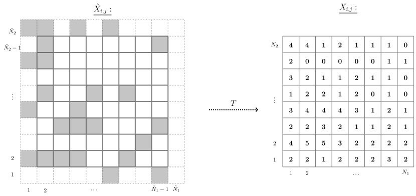
Refer to caption

Figure 5. A realization of the minesweeper related model

We present numerical results (TableΒ 1-TableΒ 8) for the described block-factor model with N~1=N~2=44subscript~𝑁1subscript~𝑁244\tilde{N}_{1}=\tilde{N}_{2}=44 (that is N1=N2=42subscript𝑁1subscript𝑁242N_{1}=N_{2}=42), m1=m2=3subscriptπ‘š1subscriptπ‘š23m_{1}=m_{2}=3 and the underlying random field generated by i.i.d. Bernoulli random variables of parameter p𝑝p (X~i,jβˆΌβ„¬β€‹(p)similar-tosubscript~𝑋𝑖𝑗ℬ𝑝\tilde{X}_{i,j}\sim{\mathcal{B}}(p)) in the range {0.1,0.3,0.5,0.7}0.10.30.50.7\{0.1,0.3,0.5,0.7\}. We also include numerical values for the corresponding i.i.d. model: N1=N2=42subscript𝑁1subscript𝑁242N_{1}=N_{2}=42, m1=m2=3subscriptπ‘š1subscriptπ‘š23m_{1}=m_{2}=3 and Xi,jβˆΌβ„¬β€‹(8,p)similar-tosubscript𝑋𝑖𝑗ℬ8𝑝X_{i,j}\sim{\mathcal{B}}(8,p).

Table 1. Block-factor: m1=m2=3subscriptπ‘š1subscriptπ‘š23m_{1}=m_{2}=3, N~1=N~2=44subscript~𝑁1subscript~𝑁244\tilde{N}_{1}=\tilde{N}_{2}=44, N1=N2=42subscript𝑁1subscript𝑁242N_{1}=N_{2}=42, 𝐩=0.1𝐩0.1\bf{p=0.1}, I​T​E​R=108𝐼𝑇𝐸𝑅superscript108ITER=10^{8}
n𝑛n S​i​mπ‘†π‘–π‘šSim A​p​p​r​o​xπ΄π‘π‘π‘Ÿπ‘œπ‘₯Approx Ea​p​psubscriptπΈπ‘Žπ‘π‘E_{app} Es​i​msubscriptπΈπ‘ π‘–π‘šE_{sim} Et​o​t​a​lsubscriptπΈπ‘‘π‘œπ‘‘π‘Žπ‘™E_{total}
29 0.828763 0.813457 0.018678 0.024528 0.043205
30 0.886702 0.875875 0.006135 0.010670 0.016805
31 0.930094 0.922997 0.001912 0.005374 0.007286
32 0.957297 0.953079 0.000628 0.003290 0.003918
33 0.974541 0.971980 0.000204 0.002239 0.002443
34 0.985523 0.984022 0.000063 0.001588 0.001651
35 0.991524 0.990718 0.000020 0.001171 0.001191
36 0.995301 0.994885 0.000006 0.000854 0.000860
37 0.997492 0.997253 0.000002 0.000617 0.000619
38 0.998668 0.998547 0.000000 0.000447 0.000447
39 0.999313 0.999272 0.000000 0.000319 0.000319
40 0.999653 0.999629 0.000000 0.000231 0.000231
41 0.999826 0.999808 0.000000 0.000164 0.000164
42 0.999916 0.999911 0.000000 0.000116 0.000116
43 0.999963 0.999959 0.000000 0.000079 0.000079
44 0.999981 0.999979 0.000000 0.000054 0.000054
45 0.999991 0.999993 0.000000 0.000037 0.000037
46 0.999995 0.999997 0.000000 0.000022 0.000022
47 0.999999 0.999999 0.000000 0.000017 0.000017
48 1.000000 0.999999 0.000000 0.000009 0.000009
Table 2. Independent: m1=m2=3subscriptπ‘š1subscriptπ‘š23m_{1}=m_{2}=3, N1=N2=42subscript𝑁1subscript𝑁242N_{1}=N_{2}=42, ℬ​(𝐧=πŸ–,𝐩=0.1)ℬformulae-sequence𝐧8𝐩0.1\bf{{\mathcal{B}}(n=8,p=0.1)}, I​T​E​R=105𝐼𝑇𝐸𝑅superscript105ITER=10^{5}
n𝑛n S​i​mπ‘†π‘–π‘šSim A​p​p​r​o​xπ΄π‘π‘π‘Ÿπ‘œπ‘₯Approx Ea​p​psubscriptπΈπ‘Žπ‘π‘E_{app} Es​i​msubscriptπΈπ‘ π‘–π‘šE_{sim} Et​o​t​a​lsubscriptπΈπ‘‘π‘œπ‘‘π‘Žπ‘™E_{total}
17 0.789376 0.788934 0.005813 0.011393 0.017206
18 0.925456 0.925186 0.000529 0.002095 0.002625
19 0.976889 0.976763 0.000045 0.000455 0.000500
20 0.993444 0.993447 0.000003 0.000105 0.000108
21 0.998288 0.998287 0.000000 0.000023 0.000024
22 0.999584 0.999583 0.000000 0.000005 0.000005
23 0.999905 0.999905 0.000000 0.000001 0.000001
24 0.999980 0.999980 0.000000 0.000000 0.000000
Table 3. Block-factor: m1=m2=3subscriptπ‘š1subscriptπ‘š23m_{1}=m_{2}=3, N~1=N~2=44subscript~𝑁1subscript~𝑁244\tilde{N}_{1}=\tilde{N}_{2}=44, N1=N2=42subscript𝑁1subscript𝑁242N_{1}=N_{2}=42, 𝐩=0.3𝐩0.3\bf{p=0.3}, I​T​E​R=108𝐼𝑇𝐸𝑅superscript108ITER=10^{8}
n𝑛n S​i​mπ‘†π‘–π‘šSim A​p​p​r​o​xπ΄π‘π‘π‘Ÿπ‘œπ‘₯Approx Ea​p​psubscriptπΈπ‘Žπ‘π‘E_{app} Es​i​msubscriptπΈπ‘ π‘–π‘šE_{sim} Et​o​t​a​lsubscriptπΈπ‘‘π‘œπ‘‘π‘Žπ‘™E_{total}
48 0.768889 0.749275 0.046577 0.053831 0.100408
49 0.844717 0.829918 0.014207 0.019702 0.033908
50 0.899398 0.889501 0.004574 0.008810 0.013384
51 0.936771 0.930795 0.001499 0.004769 0.006269
52 0.961836 0.958113 0.000485 0.002988 0.003472
53 0.977672 0.975326 0.000152 0.002045 0.002197
54 0.987307 0.985922 0.000047 0.001463 0.001510
55 0.993022 0.992251 0.000014 0.001056 0.001070
56 0.996333 0.995917 0.000004 0.000761 0.000765
57 0.998151 0.997954 0.000001 0.000539 0.000540
58 0.999091 0.998992 0.000000 0.000381 0.000381
59 0.999576 0.999522 0.000000 0.000265 0.000265
60 0.999794 0.999802 0.000000 0.000178 0.000178
61 0.999908 0.999920 0.000000 0.000115 0.000115
62 0.999965 0.999973 0.000000 0.000077 0.000077
63 0.999993 0.999991 0.000000 0.000044 0.000044
64 0.999999 0.999998 0.000000 0.000028 0.000028
65 1.000000 0.999999 0.000000 0.000017 0.000017
Table 4. Independent: m1=m2=3subscriptπ‘š1subscriptπ‘š23m_{1}=m_{2}=3, N1=N2=42subscript𝑁1subscript𝑁242N_{1}=N_{2}=42, ℬ​(𝐧=πŸ–,𝐩=0.3)ℬformulae-sequence𝐧8𝐩0.3\bf{{\mathcal{B}}(n=8,p=0.3)}, I​T​E​R=105𝐼𝑇𝐸𝑅superscript105ITER=10^{5}
n𝑛n S​i​mπ‘†π‘–π‘šSim A​p​p​r​o​xπ΄π‘π‘π‘Ÿπ‘œπ‘₯Approx Ea​p​psubscriptπΈπ‘Žπ‘π‘E_{app} Es​i​msubscriptπΈπ‘ π‘–π‘šE_{sim} Et​o​t​a​lsubscriptπΈπ‘‘π‘œπ‘‘π‘Žπ‘™E_{total}
35 0.716804 0.716395 0.012836 0.021243 0.034079
36 0.867167 0.866643 0.001951 0.005093 0.007044
37 0.943946 0.944024 0.000285 0.001409 0.001694
38 0.978505 0.978400 0.000039 0.000419 0.000457
39 0.992274 0.992262 0.000005 0.000126 0.000131
40 0.997395 0.997399 0.000001 0.000037 0.000037
41 0.999176 0.999178 0.000000 0.000010 0.000010
42 0.999753 0.999754 0.000000 0.000003 0.000003
43 0.999931 0.999931 0.000000 0.000001 0.000001
44 0.999982 0.999982 0.000000 0.000000 0.000000
45 0.999995 0.999995 0.000000 0.000000 0.000000
Table 5. Block-factor: m1=m2=3subscriptπ‘š1subscriptπ‘š23m_{1}=m_{2}=3, N~1=N~2=44subscript~𝑁1subscript~𝑁244\tilde{N}_{1}=\tilde{N}_{2}=44, N1=N2=42subscript𝑁1subscript𝑁242N_{1}=N_{2}=42, 𝐩=0.5𝐩0.5\bf{p=0.5}, I​T​E​R=108𝐼𝑇𝐸𝑅superscript108ITER=10^{8}
n𝑛n S​i​mπ‘†π‘–π‘šSim A​p​p​r​o​xπ΄π‘π‘π‘Ÿπ‘œπ‘₯Approx Ea​p​psubscriptπΈπ‘Žπ‘π‘E_{app} Es​i​msubscriptπΈπ‘ π‘–π‘šE_{sim} Et​o​t​a​lsubscriptπΈπ‘‘π‘œπ‘‘π‘Žπ‘™E_{total}
61 0.725109 0.701781 0.085110 0.093544 0.178654
62 0.828019 0.888902 0.004453 0.008665 0.013118
63 0.899560 0.888902 0.004453 0.008665 0.013118
64 0.945304 0.939436 0.001049 0.004054 0.005103
65 0.972203 0.969026 0.000235 0.002334 0.002569
66 0.986999 0.985439 0.000047 0.001460 0.001507
67 0.994506 0.993814 0.000008 0.000927 0.000935
68 0.997851 0.997605 0.000001 0.000572 0.000573
69 0.999326 0.999230 0.000000 0.000320 0.000320
70 0.999826 0.999786 0.000000 0.000171 0.000171
71 0.999968 0.999952 0.000000 0.000083 0.000083
72 1.000000 1.000000 0.000000 0.000000 0.000000
Table 6. Independent: m1=m2=3subscriptπ‘š1subscriptπ‘š23m_{1}=m_{2}=3, N1=N2=42subscript𝑁1subscript𝑁242N_{1}=N_{2}=42, ℬ​(𝐧=πŸ–,𝐩=0.5)ℬformulae-sequence𝐧8𝐩0.5\bf{{\mathcal{B}}(n=8,p=0.5)}, I​T​E​R=105𝐼𝑇𝐸𝑅superscript105ITER=10^{5}
n𝑛n S​i​mπ‘†π‘–π‘šSim A​p​p​r​o​xπ΄π‘π‘π‘Ÿπ‘œπ‘₯Approx Ea​p​psubscriptπΈπ‘Žπ‘π‘E_{app} Es​i​msubscriptπΈπ‘ π‘–π‘šE_{sim} Et​o​t​a​lsubscriptπΈπ‘‘π‘œπ‘‘π‘Žπ‘™E_{total}
50 0.741089 0.735210 0.010514 0.018002 0.028516
51 0.882209 0.880827 0.001499 0.004196 0.005695
52 0.952545 0.952389 0.000200 0.001098 0.001299
53 0.982842 0.982891 0.000024 0.000307 0.000331
54 0.994328 0.994337 0.000002 0.000084 0.000087
55 0.998282 0.998278 0.000000 0.000022 0.000022
56 0.999517 0.999518 0.000000 0.000005 0.000005
57 0.999876 0.999876 0.000000 0.000001 0.000001
58 0.999971 0.999971 0.000000 0.000000 0.000000
59 0.999994 0.999994 0.000000 0.000000 0.000000
60 0.999999 0.999999 0.000000 0.000000 0.000000
Table 7. Block-factor: m1=m2=3subscriptπ‘š1subscriptπ‘š23m_{1}=m_{2}=3, N~1=N~2=44subscript~𝑁1subscript~𝑁244\tilde{N}_{1}=\tilde{N}_{2}=44, N1=N2=42subscript𝑁1subscript𝑁242N_{1}=N_{2}=42, 𝐩=0.7𝐩0.7\bf{p=0.7}, I​T​E​R=108𝐼𝑇𝐸𝑅superscript108ITER=10^{8}
n𝑛n S​i​mπ‘†π‘–π‘šSim A​p​p​r​o​xπ΄π‘π‘π‘Ÿπ‘œπ‘₯Approx Ea​p​psubscriptπΈπ‘Žπ‘π‘E_{app} Es​i​msubscriptπΈπ‘ π‘–π‘šE_{sim} Et​o​t​a​lsubscriptπΈπ‘‘π‘œπ‘‘π‘Žπ‘™E_{total}
70 0.729239 0.705944 0.074290 0.082392 0.156682
71 0.876484 0.864370 0.006976 0.011623 0.018600
72 1.000000 1.000000 0.000000 0.000000 0.000000
Table 8. Independent: m1=m2=3subscriptπ‘š1subscriptπ‘š23m_{1}=m_{2}=3, N1=N2=42subscript𝑁1subscript𝑁242N_{1}=N_{2}=42, ℬ​(𝐧=πŸ–,𝐩=0.7)ℬformulae-sequence𝐧8𝐩0.7\bf{{\mathcal{B}}(n=8,p=0.7)}, I​T​E​R=105𝐼𝑇𝐸𝑅superscript105ITER=10^{5}
n𝑛n S​i​mπ‘†π‘–π‘šSim A​p​p​r​o​xπ΄π‘π‘π‘Ÿπ‘œπ‘₯Approx Ea​p​psubscriptπΈπ‘Žπ‘π‘E_{app} Es​i​msubscriptπΈπ‘ π‘–π‘šE_{sim} Et​o​t​a​lsubscriptπΈπ‘‘π‘œπ‘‘π‘Žπ‘™E_{total}
62.0 0.620295 0.611819 0.030328 0.042319 0.072646
63.0 0.847421 0.846730 0.002591 0.005851 0.008442
64.0 0.952524 0.952588 0.000194 0.000978 0.001172
65.0 0.987854 0.987887 0.000011 0.000168 0.000179
66.0 0.997472 0.997460 0.000000 0.000026 0.000027
67.0 0.999568 0.999568 0.000000 0.000003 0.000003
68.0 0.999943 0.999943 0.000000 0.000000 0.000000
69.0 0.999994 0.999994 0.000000 0.000000 0.000000

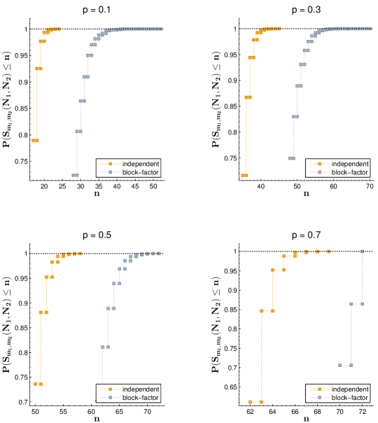
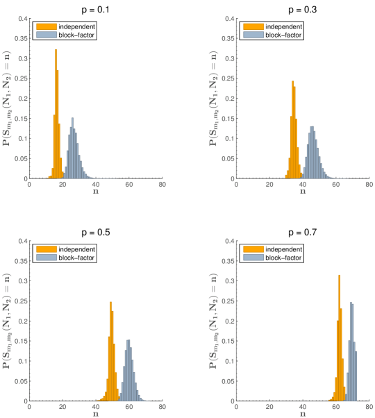
For all our results presented in the tables we used Monte Carlo simulations with 108superscript10810^{8} iterations for the block-factor model and with 105superscript10510^{5} replicas for the i.i.d. model. Notice that the contribution of the approximation error (Ea​p​psubscriptπΈπ‘Žπ‘π‘E_{app}) to the total error is almost negligible in most of the cases with respect to the simulation error (Es​i​msubscriptπΈπ‘ π‘–π‘šE_{sim}). Thus, the precision of the method will depend mostly on the number of iterations (I​T​E​R𝐼𝑇𝐸𝑅ITER) used to estimate Qu​vsubscript𝑄𝑒𝑣Q_{uv}. The cumulative distribution function and the probability mass function for the block-factor and i.i.d. models are presented in FigureΒ 6 and FigureΒ 7.

Refer to caption

Figure 6. Cumulative distribution function for block–factor and i.i.d. models

Refer to caption

Figure 7. Probability mass function for blockβˆ’-factor and i.i.d. models

4.2. Example 2: Moving Average model

In this example we consider the particular situation of an one dimensional scan statistics over a M​A​(q)π‘€π΄π‘žMA(q) model. In the two dimensional block-factor model introduced in SectionΒ 2 we consider N~2=1subscript~𝑁21\tilde{N}_{2}=1, which in particular implies that c2=1subscript𝑐21c_{2}=1 and m2=1subscriptπ‘š21m_{2}=1, x1=0subscriptπ‘₯10x_{1}=0 and x2=qsubscriptπ‘₯2π‘žx_{2}=q for qβ‰₯1π‘ž1q\geq 1 a positive integer. Let m1β‰₯2subscriptπ‘š12m_{1}\geq 2, N~1β‰₯m1+q+1subscript~𝑁1subscriptπ‘š1π‘ž1\tilde{N}_{1}\geq m_{1}+q+1 be positive integers and {X~i=X~i,1| 1≀i≀N~1}conditional-setsubscript~𝑋𝑖subscript~𝑋𝑖11𝑖subscript~𝑁1\left\{\tilde{X}_{i}=\tilde{X}_{i,1}\ |\ 1\leq i\leq\tilde{N}_{1}\right\} be a sequence of i.i.d. Gaussian random variables with known mean ΞΌπœ‡\mu and variance Οƒ2superscript𝜎2{\sigma}^{2}. We observe that N1=N~1βˆ’qsubscript𝑁1subscript~𝑁1π‘žN_{1}=\tilde{N}_{1}-q and that for each i∈{1,…,N1}𝑖1…subscript𝑁1i\in\{1,\dots,N_{1}\} the configuration matrix becomes

C(i)=(X~i,X~i+1,…,X~i+q).subscript𝐢𝑖subscript~𝑋𝑖subscript~𝑋𝑖1…subscript~π‘‹π‘–π‘žC_{(i)}=\left(\tilde{X}_{i},\tilde{X}_{i+1},\dots,\tilde{X}_{i+q}\right). (4.4)

Let the transformation T:β„³1,q+1​(ℝ)→ℝ:𝑇→subscriptβ„³1π‘ž1ℝℝT:{\mathcal{M}}_{1,q+1}({\mathbb{R}})\to{\mathbb{R}} be defined by

T​(x1,…,xq+1)=a1​x1+a2​x2+β‹―+aq+1​xq+1,𝑇subscriptπ‘₯1…subscriptπ‘₯π‘ž1subscriptπ‘Ž1subscriptπ‘₯1subscriptπ‘Ž2subscriptπ‘₯2β‹―subscriptπ‘Žπ‘ž1subscriptπ‘₯π‘ž1T(x_{1},\dots,x_{q+1})=a_{1}x_{1}+a_{2}x_{2}+\dots+a_{q+1}x_{q+1}, (4.5)

where a=(a1,…,aq+1)βˆˆβ„q+1π‘Žsubscriptπ‘Ž1…subscriptπ‘Žπ‘ž1superscriptβ„π‘ž1a=(a_{1},\dots,a_{q+1})\in{\mathbb{R}}^{q+1} a not null vector and consider the block-factor model

Xi=T​(C(i))=a1​X~i+a2​X~i+1+β‹―+aq+1​X~i+q,  1≀i≀N1.formulae-sequencesubscript𝑋𝑖𝑇subscript𝐢𝑖subscriptπ‘Ž1subscript~𝑋𝑖subscriptπ‘Ž2subscript~𝑋𝑖1β‹―subscriptπ‘Žπ‘ž1subscript~π‘‹π‘–π‘ž1𝑖subscript𝑁1X_{i}=T\left(C_{(i)}\right)=a_{1}\tilde{X}_{i}+a_{2}\tilde{X}_{i+1}+\dots+a_{q+1}\tilde{X}_{i+q},\,\,1\leq i\leq N_{1}. (4.6)

Clearly, the sequence X1,…,XN1subscript𝑋1…subscript𝑋subscript𝑁1X_{1},\dots,X_{N_{1}} forms a M​A​(q)π‘€π΄π‘žMA(q) model. Notice that the moving sums Yt=Yt,1subscriptπ‘Œπ‘‘subscriptπ‘Œπ‘‘1Y_{t}=Y_{t,1}, 1≀t≀N1βˆ’m1+11𝑑subscript𝑁1subscriptπ‘š111\leq t\leq N_{1}-m_{1}+1, can be expressed as

Yt=βˆ‘i=tt+m1βˆ’1Xi=b1​X~t+b2​X~t+1+β‹―+bm1+q​X~t+m1βˆ’1+q.subscriptπ‘Œπ‘‘superscriptsubscript𝑖𝑑𝑑subscriptπ‘š11subscript𝑋𝑖subscript𝑏1subscript~𝑋𝑑subscript𝑏2subscript~𝑋𝑑1β‹―subscript𝑏subscriptπ‘š1π‘žsubscript~𝑋𝑑subscriptπ‘š11π‘žY_{t}=\displaystyle\sum_{i=t}^{t+m_{1}-1}{X_{i}}=b_{1}\tilde{X}_{t}+b_{2}\tilde{X}_{t+1}+\dots+b_{m_{1}+q}\tilde{X}_{t+m_{1}-1+q}. (4.7)

If, for example, m1β‰₯qsubscriptπ‘š1π‘žm_{1}\geq q then the coefficients b1,…,bm1+qsubscript𝑏1…subscript𝑏subscriptπ‘š1π‘žb_{1},\dots,b_{m_{1}+q} are given by

bk={βˆ‘j=1kaj,Β k∈{1,…,qβˆ’1}βˆ‘j=1q+1aj,Β k∈{q+1,…,m1}βˆ‘j=kβˆ’m1+1kaj,Β k∈{m1+1,…,m1+q}.subscriptπ‘π‘˜casessuperscriptsubscript𝑗1π‘˜subscriptπ‘Žπ‘—,Β k∈{1,…,qβˆ’1}missing-subexpressionsuperscriptsubscript𝑗1π‘ž1subscriptπ‘Žπ‘—,Β k∈{q+1,…,m1}missing-subexpressionsuperscriptsubscriptπ‘—π‘˜subscriptπ‘š11π‘˜subscriptπ‘Žπ‘—,Β k∈{m1+1,…,m1+q}.missing-subexpressionb_{k}=\left\{\begin{array}[]{lll}\displaystyle\sum_{j=1}^{k}{a_{j}}&\mbox{, $k\in\{1,\dots,q-1\}$}\\ \displaystyle\sum_{j=1}^{q+1}{a_{j}}&\mbox{, $k\in\{q+1,\dots,m_{1}\}$}\\ \displaystyle\sum_{j=k-m_{1}+1}^{k}{a_{j}}&\mbox{, $k\in\{m_{1}+1,\dots,m_{1}+q\}.$}\end{array}\right. (4.8)

Therefore, for each t∈{1,…,N1βˆ’m1+1}𝑑1…subscript𝑁1subscriptπ‘š11t\in\{1,\dots,N_{1}-m_{1}+1\}, the random variable Ytsubscriptπ‘Œπ‘‘Y_{t} follows a normal distribution with mean 𝔼​[Yt]=(b1+β‹―+bm+q)​μ𝔼delimited-[]subscriptπ‘Œπ‘‘subscript𝑏1β‹―subscriptπ‘π‘šπ‘žπœ‡{\mathbb{E}}\left[Y_{t}\right]=(b_{1}+\dots+b_{m+q})\mu and variance V​a​r​[Yt]=(b12+β‹―+bm+q2)​σ2π‘‰π‘Žπ‘Ÿdelimited-[]subscriptπ‘Œπ‘‘superscriptsubscript𝑏12β‹―superscriptsubscriptπ‘π‘šπ‘ž2superscript𝜎2Var\left[Y_{t}\right]=\left(b_{1}^{2}+\dots+b_{m+q}^{2}\right){\sigma}^{2}. The covariance matrix Ξ£={C​o​v​[Yt,Ys]}Ξ£πΆπ‘œπ‘£subscriptπ‘Œπ‘‘subscriptπ‘Œπ‘ \Sigma=\{Cov\left[Y_{t},Y_{s}\right]\} has the entries

C​o​v​[Yt,Ys]={(βˆ‘j=1m1+qβˆ’|tβˆ’s|bj​b|tβˆ’s|+j)​σ2,Β |tβˆ’s|≀m1+qβˆ’10, otherwise.πΆπ‘œπ‘£subscriptπ‘Œπ‘‘subscriptπ‘Œπ‘ casessuperscriptsubscript𝑗1subscriptπ‘š1π‘žπ‘‘π‘ subscript𝑏𝑗subscript𝑏𝑑𝑠𝑗superscript𝜎2,Β |tβˆ’s|≀m1+qβˆ’10, otherwise.Cov\left[Y_{t},Y_{s}\right]=\left\{\begin{array}[]{ll}\displaystyle\left(\sum_{j=1}^{m_{1}+q-|t-s|}{b_{j}b_{|t-s|+j}}\right){\sigma}^{2}&\mbox{, $|t-s|\leq m_{1}+q-1$}\\ 0&\mbox{, otherwise.}\end{array}\right. (4.9)

Given the mean and the covariance matrix of the vector (Y1,…,YN1βˆ’m1+1)subscriptπ‘Œ1…subscriptπ‘Œsubscript𝑁1subscriptπ‘š11(Y_{1},\dots,Y_{N_{1}-m_{1}+1}), one can use the importance sampling algorithm developed by Naiman and Priebe [2001] (see also Malley, Naiman and Wilson [2002] and Shi, Siegmund and Yakir [2001]) to estimate the distribution of the one dimensional scan statistics S=Sm1​(N1)𝑆subscript𝑆subscriptπ‘š1subscript𝑁1S=S_{m_{1}}(N_{1}). Another way is to use the algorithm developed by Genz and Bretz [2009] to approximate the multivariate normal distribution. In this paper we adopt the importance sampling procedure.

In order to evaluate the accuracy of the approximation developed in SectionΒ 3, we consider q=2π‘ž2q=2, N1=1000subscript𝑁11000N_{1}=1000, m1=20subscriptπ‘š120m_{1}=20, X~iβˆΌπ’©β€‹(0,1)similar-tosubscript~𝑋𝑖𝒩01\tilde{X}_{i}\sim{\mathcal{N}}(0,1) and the coefficients of the moving average model (a1,a2,a3)=(0.3,0.1,0.5)subscriptπ‘Ž1subscriptπ‘Ž2subscriptπ‘Ž30.30.10.5(a_{1},a_{2},a_{3})=(0.3,0.1,0.5). In TableΒ 9 we present numerical results for the setting described above. In our algorithms we used I​T​E​Ra​p​p=106𝐼𝑇𝐸subscriptπ‘…π‘Žπ‘π‘superscript106ITER_{app}=10^{6} iterations for the approximation and I​T​E​Rs​i​m=105𝐼𝑇𝐸subscriptπ‘…π‘ π‘–π‘šsuperscript105ITER_{sim}=10^{5} replicas for the simulation.

Table 9. MA model: m1=20subscriptπ‘š120m_{1}=20, N1=1000subscript𝑁11000N_{1}=1000, Xi=0.3​X~i+0.1​X~i+1+0.5​X~i+2subscript𝑋𝑖0.3subscript~𝑋𝑖0.1subscript~𝑋𝑖10.5subscript~𝑋𝑖2X_{i}=0.3\tilde{X}_{i}+0.1\tilde{X}_{i+1}+0.5\tilde{X}_{i+2}, I​T​E​Ra​p​p=106𝐼𝑇𝐸subscriptπ‘…π‘Žπ‘π‘superscript106ITER_{app}=10^{6}, I​T​E​Rs​i​m=105𝐼𝑇𝐸subscriptπ‘…π‘ π‘–π‘šsuperscript105ITER_{sim}=10^{5}
n𝑛n S​i​mπ‘†π‘–π‘šSim A​p​p​r​o​xπ΄π‘π‘π‘Ÿπ‘œπ‘₯Approx Ea​p​psubscriptπΈπ‘Žπ‘π‘E_{app} Es​i​msubscriptπΈπ‘ π‘–π‘šE_{sim} Et​o​t​a​lsubscriptπΈπ‘‘π‘œπ‘‘π‘Žπ‘™E_{total}
11 0.582252 0.584355 0.011503 0.003653 0.015156
12 0.770971 0.771446 0.002319 0.001691 0.004010
13 0.889986 0.889431 0.000434 0.000733 0.001167
14 0.951529 0.951723 0.000073 0.000297 0.000370
15 0.980653 0.980675 0.000011 0.000113 0.000124
16 0.992827 0.992791 0.000001 0.000040 0.000042
17 0.997486 0.997499 0.000000 0.000013 0.000014
18 0.999186 0.999188 0.000000 0.000004 0.000004
19 0.999754 0.999754 0.000000 0.000001 0.000001
20 0.999930 0.999930 0.000000 0.000000 0.000000

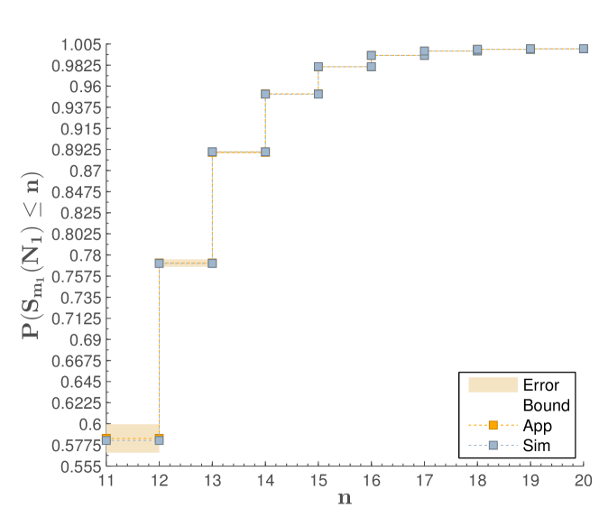
In FigureΒ 8 we illustrate the cumulative distribution functions obtained by approximation and simulation. For the approximation we present also the corresponding lower and upper bounds (computed from the total error of the approximation process (Et​o​t​a​lsubscriptπΈπ‘‘π‘œπ‘‘π‘Žπ‘™E_{total} column in TableΒ 9)).

Refer to caption

Figure 8. Cumulative distribution function for approximation and simulation along with the corresponding error under M​A𝑀𝐴MA model

5. Conclusions

In this article we derived an approximation for the two dimensional discrete scan statistic generated by a block-factor type model obtained from an i.i.d. sequence. Our method provides a sharp approximation for the high order quantiles of the distribution of the scan statistics along with the corresponding error bounds. A simulation study was included to show the accuracy of our method.

References

  • AmΔƒrioarei [2012] AmΔƒrioarei, A.: Approximation for the distribution of extremes of one dependent stationary sequences of random variables. arXiv:1211.5456v1
  • AmΔƒrioarei and Preda [2013] AmΔƒrioarei, A. and Preda, C.: Approximation for the Distribution of Three-dimensional Discrete Scan Statistic, Methodol Comput Appl Probab, DOI:10.1007/s11009-013-9382-3
  • Boutsikas and Koutras [2003] Boutsikas, M. and Koutras, M. : Bounds for the distribution of two dimensional binary scan statistics, Probability in the Engineering and Information Sciences, 17, 509–525, 2003.
  • Boutsikas and Koutras [2000] Boutsikas, M.V., Koutras, M.: Reliability approximations for Markov chain imbeddable systems. Methodol Comput Appl Probab 2, 393–412, 2000.
  • Burton, Goulet and Meester [1993] Burton, R., Goulet, M. and Meester, R.: On one-dependent processes and k-block factors. Ann. Probab., 21, 2157–2168, 1993. Processing
  • Chen and Glaz [1996] Chen, J. and Glaz, J. : Two-dimensional discrete scan statistics. Statistics and Probability Letters, 31, 59–68, 1996.
  • Darling and Waterman [1986] Darling, R., Waterman, M.: Extreme value distribution for the largest cube in a random lattice. SIAM J. Appl Math 46, 118–132, 1986.
  • Glaz, Naus and Wallenstein [2001] Glaz, J., Naus, J., Wallenstein, S.: Scan statistic. Springer, 2001.
  • Glaz, Pozdnyakov and Wallenstein [2009] Glaz, J., Pozdnyakov, V., Wallenstein, S.: Scan statistic: Methods and Applications. Birkhauser, 2009.
  • Genz and Bretz [2009] Genz, A., Bretz, F.: Computation of Multivariate Normal and T Probabilities. Springer, 2009.
  • Goerriero, Willett and Glaz [2009] Guerriero, M., Willett, P. and Glaz, J.: Distributed target detection in a sensor network using scan statistics. IEEE Transactions on Signal, 57, No. 7, 2009. Processing
  • Haiman [1999] Haiman, G.: First passage time for some stationary processes, Stochastic Processes and their Applications, 80, 231-248, 1999.
  • Haiman [2000] Haiman, G.: Estimating the distributions of scan statistics with high precision, Extremes 3:4, 349-361, 2000.
  • Haiman [2007] Haiman, G.: Estimating the distribution of one-dimensional discrete scan statistics viewed as extremes of 1-dependent stationary sequences. J. Stat Plan Infer 137, 821–828, 2007.
  • Haiman and Preda [2002] Haiman, G., Preda, C.: A new method for estimating the distribution of scan statistics for a two dimensional Poisson process. Methodology and Computing in Applied Probability 4 393–407, 2002.
  • Haiman and Preda [2006] Haiman, G., Preda, C.: Estimation for the distribution of two-dimensional scan statistics. Methodology and Computing in Applied Probability 8, 373–381, 2006.
  • Haiman and Preda [2013] Haiman, G., Preda, C.: One dimensional scan statistics generated by some dependent stationary sequences. Statistics and Probability Letters 83, 1457–1463, 2013.
  • Marcos and Marcos [2008] Marcos, R.D.L.F. and Marcos, C.D.L.F.: From star complexes to the field: open cluster families, Astrophysical Journal, 672, 342–351, 2008.
  • Malley, Naiman and Wilson [2002] Malley, J., Naiman, D., Bailey-Wilson, J.: A Comprehensive Method for Genome Scans. Human Heredity 54, 174-–185, 2002.
  • Naiman and Priebe [2001] Naiman, D., Priebe, C.: Computing Scan Statistic p Values Using Importance Sampling, with Applications to Genetics and Medical Image Analysis. J. Comp Graph Stat 10, 296–328, 2001.
  • Shi, Siegmund and Yakir [2001] Shi, J., Siegmund, D., Yakir, B.: Importance Sampling for Estimating p Values in Linkage Analysis. Journal of the American Statistical Association 102 (2007), 929–937.