An Investigation into Surface Temperature Distributions of High-B Pulsars

Abstract

Bearing in mind the application to high-magnetic-field (high-B) radio pulsars, we investigate two-dimensional (2D) thermal evolutions of neutron stars (NSs). We pay particular attention to the influence of different equilibrium configurations on the surface temperature distributions. The equilibrium configurations are constructed in a systematic manner, in which both toroidal and poloidal magnetic fields are determined self-consistently with the inclusion of general relativistic effects. To solve the 2D heat transfer inside the NS interior out to the crust, we have developed an implicit code based on a finite-difference scheme that deals with anisotropic thermal conductivity and relevant cooling processes in the context of a standard cooling scenario. In agreement with previous studies, the surface temperatures near the pole become higher than those in the vicinity of the equator as a result of anisotropic heat transfer. Our results show that the ratio of the highest to the lowest surface temperatures changes maximally by one order of magnitude, depending on the equilibrium configurations. Despite such difference, we find that the area of such hot and cold spots is so small that the simulated X-ray spectrum could be well reproduced by a single temperature blackbody fitting.

1 Introduction

Over the past few decades, our understanding of neutron stars (NSs) has been significantly progressed thanks to discoveries of several new classes of objects (see [Kaspi (2010)] for a review). In addition to the conventional “rotation-powered pulsars” (RPPs), great advances in X-ray observations such as by Chandra, XMM Newton, and Swift have led to the discovery of a garden variety of isolated NSs, which include magnetars (e.g., [Woods & Thompson (2006), Mereghetti (2008)] for reviews), high-magnetic-field (high-B) pulsars (e.g., [Ng & Kaspi (2011), Ng et al. (2012)]), X-ray-isolated neutron stars (XINSs, see [Haberl (2007)] for a review), and central compact objects (CCOs, e.g., [Gotthelf et al. (2013)]). Among them, an extreme class is magnetars including Anomalous X-ray Pulsars (AXPs) and Soft $\gamma-$ray Repeaters (SGRs), which have very large estimated magnetic fields ($B\sim 10^{14}-10^{15}$ G) and exhibit violent flaring activities (see [Rea & Esposito (2011)] for a review). Such high magnetic fields are believed to be responsible for explaining the observational characteristics (e.g., [Thompson & Duncan (1995), Thompson & Duncan (2001)]), however the origin of magnetars (whose strong fields either come from the postcollapse rapidly spinning NSs (Thompson and Duncan, 1993) or descend from the main sequence stars (Ferrario & Wickramasinghe, 2006)) and the relation to the more conventional RPPs have not yet been clarified.

The big gap between these two classes of objects has been bridged thanks to the recent discoveries of a weakly magnetized magnetar (SGR 0418+5729; Rea et al. (2010); Turolla et al. (2011)), magnetar-like bursts from a rotation-powered pulsar (PSR J1846 —0258 Gavriil et al. (2008); Ng et al. (2008)), and pulsational radio emission from magnetars (Camilo et al., 2006, 2007; Rea et al., 2012). These pieces of observational evidence lends support to a unified vision of NSs (Kaspi, 2010) that magnetars and the conventional RPPs could originate from the same population (see Ng et al. (2012); Olausen et al. (2013) for collective references therein). In this context, high-B pulsars are attracting a paramount attention, which is very likely to connect the X-ray quiet standard RPPs with very active magnetars, showing intermediate luminosities, and occasional magnetar-like activities (Perna & Pons, 2011).

In order to understand what is the underlying physics leading to the unification theory of NSs, it is of primary importance to calculate the structure and evolution of the NSs, and compare a theoretical model with observational data. Extensive studies have been performed so far in a variety of contexts (e.g., Yakovlev and Pethick (2004); Page et al. (2006) for reviews). One important lesson we have learned from accumulating observations (Zavlin, 2007; Haberl, 2007; Nakagawa et al., 2009) is that the surface temperature of isolated NSs is not spherically symmetric (1D). This demands us to go beyond 1D modeling (e.g., Greenstein & Hartke (1983); Nomoto & Tsuruta (1986); Page & Applegate (1992); Potekhin and Yakovlev (2001), and see Pethick (1992) for collective references therein) to multi-dimensional (multi-D) modeling for the evolutionary calculations.

As has been understood since Greenstein & Hartke (1983), the presence of a sufficiently strong magnetic field ($B\gtrsim 10^{10}$ G), ubiquitous such as in the envelope of a NS, leads to anisotropy of heat transport due to both classical and quantum magnetic field effects. As a result, electron thermal conductivity is strongly suppressed in the direction perpendicular to the magnetic field and increased along the magnetic field lines (Canuto and Chiuderi, 1970; Itoh, 1975), which makes the regions around the magnetic poles warmer than those around the magnetic equator (the so-called heat blanketing effect). To accurately understand the origin of the observed surface temperature anisotropy, multi-D (currently limited to axisymmetric two-dimensional (2D)) calculations of a NS have been performed extensively so far (e.g., Geppert & Rheinhardt (2002); Geppert et al. (2004); Pérez-Azorín et al. (2006); Pons and Geppert (2007); Aguilera et al. (2008); Pons et al. (2009); Viganò et al. (2013), and see collective references therein).

One of numerical difficulties of the multi-D evolutionary models comes from the fact that one needs to deal with various dissipation processes of magnetic fields working over several orders of magnitudes in the physical scales during the long-term evolution. Goldreich and Reisenegger (1992) were the first to identify the dissipation processes of the magnetic energy in the crust of an isolated NS during its evolution. On top of the ohmic decay and the ambipolar diffusion, they first proposed that the Hall drift, though non-dissipative itself, could be an important ingredient for the field decay because it can lead to dissipation through a whistler cascade of the turbulence. To unambiguously understand how the dissipation proceeds, multi-D numerical simulations focusing on electron MHD equations (EMHD, e.g., Biskamp & Welter (1989); Cho & Lazarian (2004, 2009); Takahashi et al. (2011)) are required, because the turbulent cascade from large to small scale inherent to the Hall term is essentially a non-linear process.

In step with these advances in microphysical simulations shedding light on the physics of the dissipation processes, 2D magneto-thermal evolutionary simulations have been developed with increasing sophistication, in which best neutrino processes (e.g., Yakovlev et al. (2001)) and thermal conductivities currently available are implemented (e.g., Viganò et al. (2012) for a review). Most recent code based on finite-difference schemes (Viganò et al., 2012) can handle arbitrarily large magnetic fields with the inclusion of the Hall term, which had been a big challenge in the previous code employing a spectral method (e.g., Hollerbach & Rüdiger (2002)). By computing an extensive set of such state-of-the-art evolutionary models, Viganò et al. (2013) recently pointed out that the mentioned impressive diversity of data from X-ray space missions can be explained by variations of NS’s initial magnetic field, mass and envelope composition, which is well consistent with the concept of the unification scenario.

Joining in these efforts, we investigate 2D thermal evolution of NSs in this study. Having in mind the application to high-B pulsars, we pay attention to the influence of different equilibrium configurations of NSs on the surface temperatures distributions. Since the Hall term plays an important role in the evolution of very large magnetic field ($\gtrsim 10^{14}$ G, e.g., Viganò et al. (2013)), we only take into account the effects of magnetic field decay via a simplified analytical prescription (e.g., Aguilera et al. (2008)). To solve 2D heat transport inside the NS interior out to the crust, we develop an implicit code based on a finite-difference scheme, which deals with anisotropic thermal conductivity and relevant microphysical processes in the context of a standard cooling scenario (Yakovlev et al., 2001). The equilibrium configurations of NSs are constructed in a systematic manner by employing the Tomimura-Eriguchi scheme (Tomimura and Eriguchi, 2005), in which both toroidal and poloidal magnetic fields can be determined self-consistently with the inclusion of general relativistic effect (Kiuchi and Kotake, 2008). We employ a nuclear equation of state based on the relativistic mean-field theory by Shen et al. (1998). Based on the surface temperature distributions, we discuss the properties of X-ray spectrum expected from a variety of our 2D models.

This paper is organized as follows. In Section II, we outline our initial models and numerical methods for thermal evolutions. In Sec. III, we present numerical results. Section IV is devoted to the summary and discussion.

2 Numerical Methods

2.1 Equilibrium configurations

The magnetic field configuration in the interior of NSs is poorly known from observations. Hence we adopt stationary states of magnetized stars as the initial conditions for our 2D evolutionary calculations. We employ a nuclear EOS by Shen et al. (1998) that is based on the relativistic mean-field theory. Fig. 1 shows the number fraction of each element as a function of density. Note here that zero temperature is assumed for the case of cold NSs ($T=0$). As we will discuss later, the composition and density distribution are the critical factors to determine the cooling processes. For simplicity, we leave the inclusion of hyperons as well as pions, kaons, quarks as our future work, although some recent studies suggest the existence of hyperon matter (Weissenborn et al. (2012a, b)) can explain $\sim 2M_{\odot}$ NSs (Demorest et al. (2010); Antoniadis et al. (2013)).

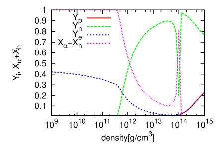
Figure 1: (Color online) Compositions for Shen EOS (Shen et al. (1998)); i.e. proton fraction $Y_{p}$ (solid line), neutron fraction $Y_{n}$ (dashed line), electron fraction $Y_{e}$ (short-dashed line). The sum of fraction of alpha particle $X_{\alpha}$ and heavy nuclei of $X_{h}$ is indicated by dotted lines.

Employing the Shen EOS, we construct equilibrium stellar configurations. The basic equations and the numerical methods for this purpose are already given in (Tomimura and Eriguchi (2005); Yoshida and Eriguchi (2006); Yoshida et al. (2006), see also Kiuchi and Kotake (2008)). Hence, we only give a brief summary for later convenience.

Assumptions to obtain the equilibrium models are summarized as follows. (1) Equilibrium models are stationary and axisymmetric. (2) The matter source is approximated by a perfect fluid with infinite conductivity. Note that this assumption is valid before magnetic field begins to decay on a timescale of $10^{6}$ yr (Pons et al., 2007). (3) There is no meridional flow of matter. (4) The magnetic axis and rotation axis are aligned.

With these assumptions, we need to specify some arbitrary parameters in the above scheme for determining equilibrium configurations. First, the toroidal magnetic field has a functional form with respect to the so-called flux function $u$ as

$$B_{\rm\phi}=\frac{a(u-u_{\rm max})^{k+1}}{R^{2}(k+1)},$$ (1)

where $a$ and $k$ are arbitrary constants to determine the magnetic field strength, and $u_{\rm max}$ is the maximum value of the flux function $u$ that depends on $R$ and the vector potential $A_{\phi}$ as $u=RA_{\phi}$. Note we employ the cylindrical coordinates $(R,\phi,z)$. Another important parameter appears in the equation of current density $j^{a}$,

$$\frac{j^{a}}{c}=\frac{\kappa}{4\pi}{B^{a}}+\rho(\mu+R^{2}\Omega\Omega^{\prime})\varphi^{a},$$ (2)

where $\mu$ is the input parameter, and other variables ($\kappa$, $\Omega\,$; angular velocity, $\rho\,$; mass density) can be determined self-consistently by solving the generalized Grad-Shafranov equation (equivalently the Maxwell equations for constructing the equilibrium configurations) and time-independent Euler equations (see Tomimura and Eriguchi (2005); Yoshida and Eriguchi (2006); Kiuchi and Kotake (2008) for more details). The only remaining parameter is the central density of a star ($\rho_{c}$).

In Table 1 we summarize the four parameters ($a$, $\mu$, $k$ and $\rho_{c}$) to obtain the equilibrium configurations. In the table, models M000 and m000 are non-magnetized models ($a=0$). The difference between them is the central density, which is higher for model M000 leading to greater (baryonic) mass ($2.20M_{\odot}$, see Table 2) than for model m00 ($1.67M_{\odot}$). As is well known, if a maximum density of a star is higher than the nuclear saturation density $\rho_{\rm nuc}\approx 2.8\times 10^{14}~{}{\rm g}~{}{\rm cm}^{-3}$, one needs to take into account a general relativistic (GR) effect. However, the fully GR approach to the magnetized equilibrium configuration has not been established yet except for the purely poloidal (Bocquet et al., 1995; Cardall et al., 2001) or toroidal fields (Kiuchi & Yoshida, 2008). Therefore we employ an approximate, post-Newtonian method proposed by Kiuchi and Kotake (2008).

Back to Table 1, models mauk, maUk, MaUk and mAUk, are all magnetized models. In Table 2, several important quantities of the equilibrium models are summarized, i.e., the mass $M$, the radius $R$, the poloidal magnetic field at the pole $B_{p}$, the magnetic filed in the center $B_{c}$, the ratio of the total magnetic field energy to the gravitational energy $H/|W|$, and the ratio of the maximum magnetic field for the toroidal component to that for the poloidal one $B_{\phi,\rm{max}}/B_{p,\rm{max}}$. For all the magnetized models, $B_{p}$ is set to take $\sim 10^{13}$ G, which is reconciled with high-B pulsars. Since $H/|W|$ are quite small ($\ll 1$), the equilibrium configurations are not affected by the Lorentz force (see, however Yasutake et al. (2010) for ultra-strong field ($B\gtrsim 10^{17}$ G) case). The ratio of $B_{t,\rm{max}}/B_{p,\rm{max}}$ is in line with results from recent MHD simulations (Braithwaite and Spruit (2004)), showing that stable configurations require the coexistence of both poloidal and toroidal components, approximately of the same strength. As an experimental point of view, we compute two extreme cases for models maUS and mSUK, which do not satisfy the stability condition.

We checked the convergence of the presented results by doubling the number of mesh points from the standard set of radial and angular direction mesh points of 100 $\times$ 100. We set the uniform zones in the polar direction while non-uniform zones in the radial direction to describe the density profile and the particle compositions in the crusts precisely. Here, the zone-interval in the radial direction is, $dr_{n}=dr_{0}\times q^{n-1}$ from the center, where the indent $n$ is the zone number measured from the center. The constant $dr_{0}$ denotes the maximum grid interval that is related to the maximum equatorial radius $R_{\rm eq}$ of each model as $dr_{0}=(R_{\rm eq}-1)/(n_{\rm max}-1)$. Here, $n_{\rm max}$ denotes the maximum zone-number, set as $n_{\rm max}=100$ and $q=0.99$ in this study. The minimum grid interval is of the order of one meter in all our simulations, which is small enough to calculate the crust of a NS. By checking the virial identities (Cowling, 1965) for all the models, we confirm that the typical values are of the orders of magnitude $\lesssim 10^{-3}$, which are almost the same for the polytropic EOS case (Tomimura and Eriguchi, 2005; Yoshida and Eriguchi, 2006). In general, the convergence is known to become much worse for realistic EOS because their adiabatic index is not smooth especially near $\rho_{\rm nuc}$. In this respect, our numerical scheme works well.

Table 1: Models with parameters to determine magnetic field distributions. Note that the unit of $a$ is depends on the value of $k$ through Eq.(1). As for the values of $a$, $\mu$, $k$ in this table, we adopt the geometrical units as in previous studies (Tomimura and Eriguchi, 2005; Yoshida and Eriguchi, 2006; Kiuchi and Kotake, 2008).

Models	$\rho_{c}$	$a$	$\mu$	$k$
	[1014 g cm-3]
M000	12.00	0.0	0.00 $\times 10^{0}$	0.00
m000	6.00	0.0	0.00 $\times 10^{0}$	0.00
mauk	6.00	70.0	1.00 $\times 10^{-5}$	1.00$\times 10^{-1}$
maUk	6.00	70.0	1.00 $\times 10^{-4}$	1.00$\times 10^{-1}$
MaUk	12.00	70.0	1.00 $\times 10^{-4}$	1.00$\times 10^{-1}$
mAUk	6.00	100.0	1.00 $\times 10^{-4}$	1.00$\times 10^{-1}$
maUS	6.00	70.0	1.00 $\times 10^{-4}$	1.00$\times 10^{0}$
mSUK	6.00	5000.0	1.00 $\times 10^{-4}$	8.00$\times 10^{-1}$

Table 2: Summary of initial Models (see text for the definition of variables).

Models	$M$	$R$	$B_{p}$	$B_{c}$	$H/|W|$	$B_{t,\rm{max}}/B_{p,\rm{max}}$
	[$M_{\odot}$]	[km]	[1014 G]	[1014 G ]
M000	2.20	12.9	-	-	-	-
m000	1.67	14.3	-	-	-	-
mauk	1.67	14.4	0.05	0.21	1.09 $\times 10^{-10}$	0.57
maUk	1.67	14.3	0.48	2.11	1.26 $\times 10^{-8}$	0.75
MaUk	2.20	12.9	0.72	3.22	8.49 $\times 10^{-9}$	0.65
mAUk	1.67	14.2	0.45	2.26	1.49 $\times 10^{-8}$	1.04
maUS	1.67	14.2	0.42	1.76	5.73 $\times 10^{-9}$	2.80$\times 10^{-6}$
mSUK	1.67	14.3	0.44	1.84	6.30 $\times 10^{-9}$	0.13

Figure 2 shows equilibrium configuration for our fiducial model (maUk). As already mentioned, the assumed field strength is not so dynamically strong that the density and composition distributions are essentially spherical ($M$ and $R$ in Table 2 are hardly dependent on the field strength). Therefore the density distribution for model maUK is similar to the remaining models, given the same central density.

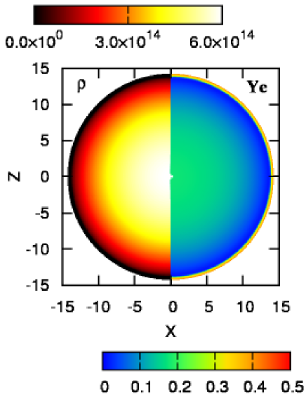
Figure 2: (Color online) The density profile $\rho$[g cm^-3], and the electron fraction $Y_{e}$ for model maUk in Table I. Note that the distributions are all similar to the remaining models m000, mauk, mAUk, and maUS.

The left and right panels of Figure 3 show the distribution of magnetic field for model maUK and mSUK, respectively, with respect to the lateral ($|B_{\theta}|$, left top), azimuthal ($|B_{\phi}|$, left bottom), radial component ($|B_{r}|$, right top), and the sum ($B=\sqrt{B_{r}^{2}+B_{\theta}^{2}+B_{\phi}^{2}}$, right bottom, all in the absolute value). Note again that the magnetic distribution is dependent on the four parameters ($\rho_{c}$, $a$, $\mu$, and $k$). From the right panel, it can be seen that the toroidal magnetic field ($|B_{\phi}|$ amplified by a factor of 5, bottom left panel) is dominant over the poloidal components (e.g., the top panels for $|B_{\theta}|$ and $|B_{r}|$) in the vicinity of the equatorial plane out to $\sim 7$ km in radius. The dominance of the toroidal fields in the vicinity of the outer regions is common to model maUk (right panel of Figure 3). The most remarkable difference between the left and right panel in Figure 3 is the distribution of the toroidal component $|B_{\phi}|$, which is confined in a narrow region for model maUk (seen as a half-circle colored by yellow in the $|B_{\phi}|$ plot) at a radius of $\sim 14$ km in the vicinity of the equatorial plane. This difference comes from the parameter $k$. Smaller $k$ makes the distribution of $|B_{\phi}|$ more compact as seen in the left panel. This feature is common to models with smaller $a$ in Table 1, that is, mauk, MaUk, and maUS.

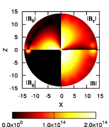
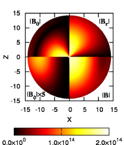
Figure 3: (Color online) The strengths of initial toroidal, poloidal, and total magnetic field; $|B_{\phi}|$, $|B_{p}|$, and $|B|$ in unit [10¹⁴ G] (see text for the definition) for model maUk (left panel) and mSUK (right panel), respectively. Note in the right panel that the strength of toroidal magnetic field, $|B_{\phi}|$, is multiplied by a factor of 5 for visualization.

2.2 Thermal evolution

Taking GR effects into account, we employ a spherically symmetric metric given by the equation (Misner et al., 1973)

$$ds^{2}=-e^{2\phi}dt^{2}+e^{2\Lambda}dr^{2}+r^{2}d\Omega^{2}.$$ (3)

Under this background metric, the thermal evolution of a NS can be described by the energy balance equation (e.g., Aguilera et al. (2008)),

$$c_{v}e^{\phi}\frac{\partial T}{\partial t}+\nabla\cdot(e^{2\phi}{\mbox{\boldmath$F$}})=e^{2\phi}(H-L),$$ (4)

where $c_{v}$ is the specific heat capacity, $T$ is the temperature, $H$ and $L$ is the energy loss and gain by neutrino emission and by the Joule heating, respectively. In the diffusion limit, the heat flux (${\mbox{\boldmath$F$}}=(F_{r},F_{\theta})$) can be expressed as

$${F_{r}} = -e^{-\phi}(\kappa_{rr}e^{-\Lambda}\partial_{r}\tilde{T}+\frac{\kappa_{r\theta}}{r}e^{-\Lambda}\partial_{\theta}\tilde{T}),$$ (5)

$${F_{\theta}} = -e^{-\phi}(\kappa_{\theta r}e^{-\Lambda}\partial_{r}\tilde{T}+\frac{\kappa_{\theta\theta}}{r}e^{-\Lambda}\partial_{\theta}\tilde{T}),$$ (6)

where $\kappa$ is the total thermal conductivity tensor and $\tilde{T}$ is the red-shifted temperature ($\tilde{T}=e^{\phi}T$). The dominant contribution to $\kappa$ comes from electrons (see Geppert et al. (2004); Page et al. (2007); Aguilera et al. (2008)), which can be written as

$$\kappa_{e} = \kappa_{e}^{\perp}\Biggl{[}{\mbox{\boldmath$E$}}$$

$$+ (\omega_{B}\tau)^{2}\left(\begin{array}[]{ccc}b_{rr}&b_{r\theta}&b_{r\phi}\\ b_{\theta r}&b_{\theta\theta}&b_{\theta\phi}\\ b_{\phi r}&b_{\phi\theta}&b_{\phi\phi}\end{array}\right)+\omega_{B}\tau\left(\begin{array}[]{ccc}0&b_{\phi}&-b_{\theta}\\ -b_{\phi}&0&b_{r}\\ b_{\theta}&-b_{r}&0\end{array}\right)\Biggr{]},$$

where $\kappa_{e}^{\perp}$, $\omega_{B}$, and $\tau$ are the electron thermal conductivity orthogonal to the magnetic field, the gyro-frequency ($\omega_{B}=eB/m_{e}^{*}c$ with $m_{e}^{*}$ being the effective electron mass), and the electron relaxation time (Urpin & Yakovlev, 1980). Here, $E$ is the identity matrix, and $b_{r}$, $b_{\theta}$, $b_{\phi}$ denotes the radial, lateral, and azimuthal component of the unit vector in the direction of the magnetic field, respectively. We employ a public code to calculate these kinematic coefficients in the crust. For the inner core, we adopt the formula in Gnedin and Yakovlev (1995).

Concerning the heat capacity ($c_{v}$ in Eq. (4)), we assume that electrons are degenerate, and baryons are non-relativistic (Aguilera et al. (2008)). In the crust, the heat capacity is provided by electrons, ions, and free neutrons. We ignore the ion contribution on the heat capacity because the contribution is small. For simplicity, we do not take the effect of superfluidity into account.

Regarding the cooling term $L$ in Eq.(4), we follow the so-called standard cooling scenario (Yakovlev et al. (2001) for a review), in which the total cooling rate is dominated by slow processes in the core, such as by modified Urca and nucleon-nucleon Bremsstrahlung (Yakovlev and Levenfish, 1995; Heansel et al., 1996). As a first step, we think the consideration of the minimal cooling scenario (Page et al., 2004) or enhanced cooling scenario (Lattimer et al., 1991; Prakash, 1992; Takatsuka and Tamagaki, 2004) as an important extension as a sequel of this study.

As for the magnetic field decay, we only take into account the Ohmic dissipation, because in our case ($B_{0}\sim 10^{13}$ G) the Hall term plays an only minor role. For simplicity, we assume that the field geometry is fixed and the evolution is included only in the normalization $B$ as (Aguilera et al., 2008)

$$B=B_{0}\,{\rm exp}\,(-t/\tau_{{\rm Ohm}}),$$ (8)

where $B_{0}$ is given by the initial equilibrium configurations, and the Ohmic decay timescale ($\tau_{{\rm Ohm}}$) is set as $10^{6}$ yr (Pons et al., 2007) in all the models. Simple as it is, such a prescription is known to be able to reproduce qualitatively results from more detailed simulations (Pons and Geppert, 2007). The heating rate ($H$) in Eq.(4) is given by the integral of $H=\int\Delta B^{2}/8\pi~{}dV$, where $\Delta B\equiv B^{n+1}-B^{n}$ denotes the decrease of the field strength in each computational timestep (between $n+1$ and $n$ steps). Note that for a middle-age NS of $10^{3}-10^{5}$ yr, to which we pay attention in this work, the Ohmic decay does not significantly affect the thermal evolution.

Here, let us estimate the diffusion timescale $\tau_{D}$ from Eq. (4). $\tau_{D}$ is proportional to $\sim c_{v}^{\prime}(\Delta x)^{2}/\kappa^{\prime}$, where $c_{v}^{\prime}$, $\Delta x$, and $\kappa^{\prime}$ are typical values for the heat capacity, the grid interval, and the thermal conductivity. Taking typical values in the core of a NS, such as $c_{v}^{\prime}\sim 10^{20}$ erg cm ^-3 K^-1, $\Delta x\sim 10^{3}$ cm, and $\kappa^{\prime}\sim 10^{23}$ erg K${}^{-1}\,{\rm s}^{-1}\,{\rm cm}^{-1}$, the diffusion time scale is estimated as $\tau_{D}\sim 10^{3}$ s. Since the evolution timescale of a NS ($\sim 10^{4}-10^{6}$ years) is much longer than the diffusion timescale, an implicit scheme is needed to solve Eq. (4). In doing so, we take an operator splitting method. The second term in Eq. (4) includes the cross terms of second derivatives such as $\partial_{r}\partial_{\theta}$ and $\partial_{\theta}\partial_{r}$, which is not straightforwardly handled by a standard matrix inversion scheme. We treat these terms as a source term to get a convergent solution (see Appendix A for more details). Finally, we employ a phenomenological formula to estimate the surface temperature $T_{s}$ from the temperature at the bottom of the envelope $T_{b}$ (Potekhin and Yakovlev, 2001) (e.g., Eq. (31,32) in Aguilera et al. (2008)), in which the density at the bottom of the envelope is set as $10^{9}$ g cm^-3.

3 Result

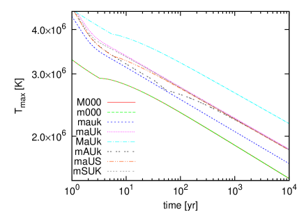
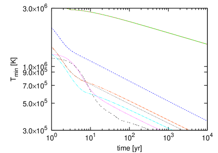
Figure 4: (Color online) Cooling light curves for all the computed models. Left and right panel shows the evolutions of the maximum ($T_{\rm max}$) and minimum ($T_{\rm min}$) surface temperatures (see text for more details). Note the difference of the temperature scale in each panel.

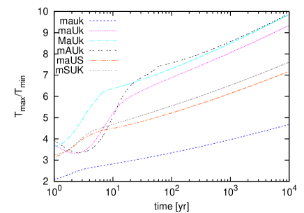
Figure 5: Time evolution of the ratio of $T_{\rm max}$ to $T_{\rm min}$ for all the magnetized models.

Due to the mentioned heat blanketing effect, the surface temperature has its maximum ($T_{\rm max}$) and minimum ($T_{\rm min}$) in the vicinity of the magnetic poles and equator for our 2D evolutionary models with magnetic fields. The left and right panels of Figure 4 show the evolution of $T_{\rm max}$ and $T_{\rm min}$ for all the computed models, respectively. Since the characteristic age for high-B pulsars is estimated as $10^{3-5}$ yr from observations (e.g., Ng et al. (2012)), we focus on the evolution up to $t_{\rm end}=10^{4}$ yr in this paper. Before going into detail, let us compare our results with Aguilera et al. (2008), especially with their Figure 13 (central panel) for their PC model, in which a similar field strength to our model maUk is employed with the use of the standard cooling processes. The temperature of the hot spot for our model maUk (e.g., pink dashed-line in the left panel of Figure 4) drops about 50 % from the birth ($T_{\rm max}$ = $4.4\times 10^{6}$ K) to the age of $10^{3}$ yr ($T_{\rm max}=2.4\times 10^{6}$ K), while the PC model Aguilera et al. (2008) drops about 40 % for the same timescale (e.g., from $T_{\rm max}\sim 10^{6.5}$ K to $\sim 10^{6.1}$ K, purple line in their figure). Therfore, our results are in good agreement with previous study, granted that similar field strength and microphysics are employed (e.g., Aguilera et al. (2008)).

Figure 5 shows that the contrast ratio of $T_{\rm max}$ to $T_{\rm min}$ for the magnetized models at $t_{\rm end}$ ranges from $\sim$ 5-10, while the contrast ratio is unity for non-magnetized models (M000, m000). In our magnetized models, the lowest and highest contrast ratio (4.86 and 10.0) is obtained for our most weakly and strongly magnetized model (mauk and mAUk), respectively (e.g., $H/|W|$ in Table 2). Note that these values are quantitatively in good agreement with previous results in which more detailed cooling processes and heat transport scheme than ours were employed (Aguilera et al. (2008)). It should be mentioned that the contrast ratio does not depend solely on the magnetized parameter $H/|W|$ but also on the configuration of the magnetic field. For example, the contrast ratio for model MaUk is larger than that for model maUk, although $H/|W|$ is smaller for model MaUk.

Note here that the initial mass hardly affects the contrast ratio. In fact, the surface temperatures for models m000 and M000 are degenerate as seen from the both panels in Fig 4. This is not surprising because we assume the standard cooling scenario. The implementation of another cooling scenario may break the degeneracy, but this is beyond the scope of this work as we mentioned earlier. Note also that even without the magnetic fields, rapid rotation can lead to anisotropic surface temperature distributions (Negreiros et al., 2012), which also needs further investigation.

In the above results, we paid attention only to the surface temperatures in the hot ($T_{\rm max}$) and cold ($T_{\rm min}$) spots, but the average temperature should be between them. Since the surface temperature is often estimated by a black-body fitting to the observed X-ray spectrum, we move on to calculate spectra from our 2D evolutionary models. Recently, some observations suggest that a two temperature black-body (2BB-) fitting (i.e., cold $\bar{T}_{C}$ and hot $\bar{T}_{H}$ component) is needed to explain observed spectra for magnetars (Nakagawa et al., 2009). Based on our results, we exploratory discuss how the spectrum could be in the case of high-B pulsars.

By integrating the surface fluxes with an assumption of the Plank law, Fig. 6 shows the simulated X-ray spectrum for model maUk (left panel) and mSUK (right panel) at 10⁴ yr. We assume the distance to the source as $D$= 1.0 kpc in the following. In the figure, we set the inclination angle $\theta$ as $\theta=0^{\circ}$, namely an equatorial observer is assumed. We will discuss the dependence of the inclination angle later.

In the figure, the cross dotted points denote the results calculated from our 2D evolutionary models (labeled as “result”) that include contribution to the spectrum from all the regions on the NS surface. To reconstruct the total spectrum (cross dotted points) either from a single or two temperature BB fitting, the dashed green line ($\bar{T}_{H}$), the dashed blue line ($\bar{T}_{C}$), and the sum ($\bar{T}_{H}+\bar{T}_{C}$) represents the spectrum for each component. Here, we determine $\bar{T}_{C}$ and $\bar{T}_{H}$ to get the best $\chi$-square fitting to the total spectrum (labeled by “result”) by changing the area-weighted spectrum with respect to the cold (blue dashed line) and hot (green dashed line) component. The left panel shows that the single BB-fitting ($\bar{T}_{H}$) is enough to reconstruct the X-ray spectrum for model maUK, although $T_{\rm max}$ is almost 10 times higher than $T_{\rm min}$ as shown in Fig 5. These features are also similar to other models (mauk, MaUk and mAUk). This indicates that the X-ray spectrum from our standard 2D models (with the coexistence of both poloidal and toroidal components) and also with the assumption of the standard cooling processes can be reconstructed by a single BB fitting. On the other hand, the right panel is from one of our extreme cases (model mSUK), which shows that the two component BB fitting is needed.

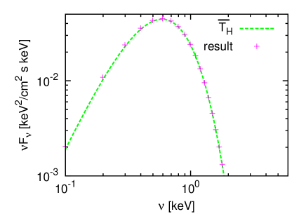
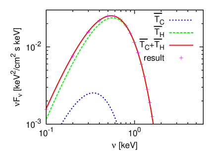
Figure 6: (Color online) Expected X-ray spectrum calculated for models maUk (left panel) and mSUK (right panel) after 10⁴ yr. Here we assume the inclination angle from the equatorial plane of observer is $\theta=0^{\circ}$. The dashed lines labeled as “result” show the estimated spectra from our 2D evolutionary models (see text for more details). The lines labeled as $\bar{T}_{C}$, $\bar{T}_{H}$, $\bar{T}_{C}+\bar{T}_{H}$), are the spectra of the hot spot, the cold spot, and the sum estimated by a single- or two- temperature BB fitting to the cross dotted points (see the text for more details).

To better understand the reason, we present in Fig. 7 the surface temperature distribution for a pair of models (model maUk (left panel ) and mSUK (right panel)). In both of the models, cold (colored by blue in the equator) and hot (yellow) spots can be seen, however, the area of the cold spot is confined in much narrow region for model maUk (left) than for model mSUK (right). As already mentioned, this is because the toroidal magnetic field $B_{\phi}$ is confined in a narrow region for model maUK (e.g., in the left panel Fig. 3), which is vice versa for model mSUK (the right panel). This is the reason why the spectrum from model maUk can be well fitted by a single temperature component, while two component fitting is needed for model mSUK. Our results present supporting evidence for previous investigations (Pérez-Azorín et al. (2006); Geppert et al. (2006)) that the temperature distribution depends primarily on the magnetic field distribution.

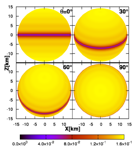
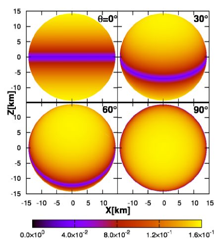
Figure 7: (Color online) Surface temperature in unit of keV for models maUk (left panel) and mSUK (right panel) after 10⁴ years as a function of the viewing angle $\theta$.

Table 3 summarizes the ratio of the surface area of the hot regions to the total surface area as a function of the inclination angle ($\theta=0^{\circ},30^{\circ},60^{\circ},$ and $90^{\circ}$) for all the models. Clearly, our four standard models (mauK, maUk, MaUk, mAUk) show a clear dominance of the hot areas over the cold areas (the ratio being greater than 0.5), while the ratio approaches to 0.5 for the two extreme cases (models maUS and mSUK) especially seen from equator ($\theta=0^{\circ}$). This again indicates that the simulated spectrum from our 2D models can be represented by a single temperature BB fitting. On the other hand, if the two temperature BB fitting would be required for a high-B-pulsar class field strength ($B_{\rm surface}\approx 10^{13}$ G), it might suggest the existence of larger cold spots (models maUS and mSUK). We speculate that this could possibly give some hints to the intrinsic field configuration (e.g., Figs. 3 and 7).

Table 3: The ratio of the area of the hot spot to that of the total NS surface.

Name	$0^{\circ}$	$30^{\circ}$	$60^{\circ}$	$90^{\circ}$
mauk	0.807	0.820	0.879	0.879
maUk	0.854	0.866	0.912	0.938
MaUk	0.715	0.722	0.759	0.801
mAUk	0.889	0.901	0.939	0.971
maUS	0.581	0.612	0.733	0.782
mSUK	0.553	0.588	0.717	0.769

Finally we summarize $\bar{T}_{C}$ and $\bar{T}_{H}$ in Table 4 for all the models as a function of some selected inclination angle. In this table, the intrinsic minimum temperature $T_{\rm min}$ and the maximum temperature $T_{\rm max}$ are given as a reference. Changing the inclination angle from the equator ($\theta=0^{\circ}$) to the pole ($\theta=90^{\circ}$, see from left to right in Table 4), $\bar{T}_{H}$ commonly increases, because the cold region in the equator is obscured for a polar observer (see Fig.7). Though all the models share a similar temperature contrast between $\bar{T}_{C}$ and $\bar{T}_{H}$, the ratio of the area (Table 3) of the two spots holds the key to determine whether the single or two component fitting is more preferential.

Table 4: Temperature of cold spot and hot spot, and average temperature given by the two component BB fittings as a function of the inclination angle. All units are in [keV]. In non-magnetized models (M000, m000), $\bar{T}_{C}$ and $\bar{T}_{H}$ is not given (–) simply because the surface temperature is uniform.

Name	$T_{\rm min}$	$T_{\rm max}$	$\bar{T}_{C}(0^{\circ})$	$\bar{T}_{H}(0^{\circ})$	$\bar{T}_{C}(30^{\circ})$	$\bar{T}_{H}(30^{\circ})$	$\bar{T}_{C}(60^{\circ})$	$\bar{T}_{H}(60^{\circ})$	$\bar{T}_{C}(90^{\circ})$	$\bar{T}_{H}(90^{\circ})$
M000	0.131	0.131	-	-	-	-	-	-	-	-
m000	0.131	0.131	-	-	-	-	-	-	-	-
mauk	0.028	0.136	0.087	0.128	0.088	0.130	0.092	0.132	0.121	0.134
maUk	0.017	0.159	0.095	0.150	0.097	0.152	0.101	0.154	0.129	0.155
MaUk	0.019	0.188	0.077	0.176	0.077	0.177	0.158	0.180	0.171	0.181
mAUk	0.016	0.161	0.094	0.155	0.095	0.155	0.098	0.156	0.128	0.157
maUS	0.022	0.157	0.088	0.144	0.090	0.147	0.095	0.149	0.111	0.151
mSUK	0.021	0.158	0.087	0.144	0.089	0.147	0.094	0.149	0.109	0.151

4 Summary and Discussions

Bearing in mind the application to high-B pulsars, we have investigated 2D thermal evolutions of NSs. We paid particular attention to the influence of different equilibrium configurations on the surface temperature distributions. The equilibrium configurations were constructed in a systematic manner, in which both toroidal and poloidal magnetic fields are determined self-consistently with the inclusion of GR effects. To solve the 2D heat transfer inside the NS interior out to the crust, we have developed an implicit code based on a finite-difference scheme that deals with anisotropic thermal conductivity and relevant cooling processes in the context of a standard cooling scenario. In agreement with previous studies, the surface temperatures near the pole become higher than those in the vicinity of the equator as a result of the heat-blanketing effect. Our results showed that the ratio of the highest to the lowest surface temperatures changes maximally by one order of magnitude, depending on the equilibrium configurations. Despite such inhomogeneous temperature distributions, we found that the area of such hot and cold spots is so small that the simulated X-ray spectrum could be well reproduced by a single temperature BB fitting. We speculated that if a two-component BB fitting is needed to account for the observed spectrum, the toroidal magnetic field could be more widely distributed inside the NS interior than for models that only require a single temperature BB fitting.

Comparing with the state-of-the-art 2D models (Geppert & Rheinhardt, 2002; Geppert et al., 2004; Pérez-Azorín et al., 2006; Pons and Geppert, 2007; Aguilera et al., 2008; Pons et al., 2009; Viganò et al., 2013), this study that is our first attempt to join in the NS evolutionary calculations have a number of caveats to be improved. First of all, we only took into account the Ohmic dissipation for simplicity. On the timescale of 10⁴ yr explored in this study, it would not have any significant effects on the thermal evolution, however, the inclusion of the Hall effect and ambipolar diffusion (e.g., Aguilera et al. (2008); Viganò et al. (2013)) is inevitable for studying the subsequent evolution to compare with observations. If direct Urca processes mediated by hyperons were taken into account (Lattimer et al., 1991; Prakash, 1992), the neutrino luminosity could be significantly enhanced (by 5-6 orders of magnitudes) compared to that of the standard cooling scenario. To test the minimal cooling and enhanced cooling scenarios is also a major undertaking. Superfluidity and superconductivity should be included, which should modify the heat capacity and neutrino emissivities (Kaminker et al., 2001; Andersson et al., 2005; Lander et al., 2012), and provide a new heat source in the crust (Tsuruta et al., 2009). Regarding the equilibrium configuration, the electric current is assumed to vanish at the surface in the present scheme. The updated numerical scheme recently proposed by Fujisawa et al. (2012) can handle the non-vanishing toroidal component there, which should affect the surface temperature distributions. We assumed that the magnetic axis is aligned with the rotational axis. To accurately deal with a misalignment that is thought to be a general feature of pulsars, we have to construct 3D equilibrium configurations, the numerical method of which has not been established yet.

A comparison with observations is one of the most important issues in the theoretical study of the thermal evolutions of NSs. Based on the state-of-the-art 2D models including both elaborate cooling rates and field-decay processes, Perna et al. (2013) have recently investigated the X-ray specta and pulse profiles for a variety of initial magnetic field configurations. They pointed out that the simulated pulse profiles are sensitive to the field configurations (e.g., the dominance between the toroidal and poloidal fields). Owing to the alignment of the rotational axis and the magnetic axis in our 2D models, such analysis is unfortunately beyond the scope of this work. In addition to the required improvements for this work (e.g., simplified treatment of field decay and cooling processes), more accurate prediction of the X-ray spectra is mandatory, in which effects of (energy-dependent) interstellar absorption, light deflection, and gravitational redshift are taken into account as in Perna et al. (2013). At the very least (before we will tackle on this subject in the future), let us note that the intrinsic cooling curves of our models (namely without the observational corrections) are qualitatively consistent with the ones in Perna et al. (2013). The upper panel of Figure 1 in Perna et al. (2013) shows the cooling curve from one of their representative models, in which a purely poloidal field ($B_{0}=10^{13}$ G) is assumed and similar microphysics (such as the cooling processes, thermal conductivity, heat capacity, and EOS) is taken as those in this work. As shown, our models (the left panel of Figure 7 in this work) reproduce similar results, in which the hot and cold spots appear on the magnetic poles and equatorial regions, respectively.

Keeping our efforts to improve these important ingredients, our final goal is to construct a fully self-consistent simulation, in which the stellar configuration is determined in a self-consistent manner under the influence of the magnetic field decay, heating and cooling processes . This study, in which we developed a new code including equilibrium configurations (albeit employing a very crude approximation of the microphysics and field decay treatment) is nothing but a prelude, however, an important trial for us to take a very first step to the long and winding road.

We would like to thank K. Kiuchi, S. Yamada, Y.Eriguchi and K. Makishima for fruitful discussions. NY is also grateful to D. Viganò, J.A. Pons, and J.A. Miralles for their warm hospitality during his stay in the University of Alicante and for their useful and insightful comments on this work. This study was supported in part by the Grants in Aid for the Scientific Research from the Ministry of Education, Science and Culture of Japan (no. 2510-5510, 23540323, 23340069, and 24244036).

Appendix A An implicit scheme for 2D thermal diffusion calculations

We briefly summarize an implicit scheme for 2D evolutionary calculations developed in this work. Fig. 8 illustrates spatial positions of a given point on the computational domain in our 2D code. The index $i$ and $j$ denotes the number of radial and lateral grid, respectively. Scalar valuables such as density ($\rho_{i,j}$), heat capacity (${c_{v~{}i,j}}$), redshift ($e^{\phi}_{i,j}$), temperature ($T_{i,j}$), and thermal conductivity ($\kappa_{i,j}$) are defined at the center of the grid, while vector valuables such as the thermal flux are defined at the cell boundary ($F_{i+1/2,j+1/2}$). The fluxes in the 2D computations consist of the following four components,

$$F_{rr} = -e^{-\phi}(\kappa_{rr}e^{-\Lambda}\partial_{r}\tilde{T}),$$ (9)

$$F_{r\theta} = -e^{-\phi}(\frac{\kappa_{r\theta}}{r}e^{-\Lambda}\partial_{\theta}\tilde{T}),$$ (10)

$$F_{\theta r} = -e^{-\phi}(\kappa_{\theta r}e^{-\Lambda}\partial_{r}\tilde{T}),$$ (11)

$$F_{\theta\theta} = -e^{-\phi}(\frac{\kappa_{\theta\theta}}{r}e^{-\Lambda}\partial_{\theta}\tilde{T}).$$ (12)

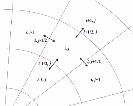
Figure 8: Schematic picture of each numbering to the grids. Each vector shows the thermal flux for $F_{rr}$ or $F_{\theta\theta}$. The other fluxes $F_{r\theta}$ and $F_{\theta r}$ are orthogonal to them, although we do not show in this figure.

Fixing hydrodynamic valuables such as density, pressure, and gravity as a background, we solve the diffusion equation (Eq. 4) by an operator-splitting method.

We solve the time evolution separately with the radial direction, the lateral direction, and the source term, respectively. The evolution regarding the radial and lateral advection can be expressed, respectively as

$$\{c_{v}e^{\phi}\}_{i,j}^{l+1} \frac{T_{i,j}^{l+1}-T_{i,j}^{l}}{\Delta t}~{}dV_{i,j}$$

$$= -\frac{\{e^{2\phi}F_{rr}\}_{i+1/2,j}^{l+1}\{dS_{r}\}_{i+1/2,j}}{dr_{i+1/2}}$$

$$+\frac{\{e^{2\phi}F_{rr}\}_{i-1/2,j}^{l+1}\{dS_{r}\}_{i-1/2,j}}{dr_{i-1/2}}$$

and

$$\{c_{v}e^{\phi}\}_{i,j}^{l+1} \frac{T_{i,j}^{l+1}-T_{i,j}^{l}}{\Delta t}~{}dV_{i,j}$$

$$= -\frac{\{e^{2\phi}F_{\theta\theta}\}_{i,j+1/2}^{l+1}dS_{i,j+1/2}}{r_{i}~{}d\theta}$$

$$+\frac{\{e^{2\phi}F_{\theta\theta}\}_{i,j-1/2}^{l+1}dS_{i,j-1/2}}{r_{i}~{}d\theta},$$

where $dr_{i+1/2}=r_{i+1}-r_{i}$ is the radial grid interval, the index $l$ is the number of arbitral timestep, $d\theta$ is an equidistant angular grid, $dV_{i,j}$ is a differential volume, and $\{dS_{r}\}_{i+1/2,j}$ is the surface area between grid $(i,j)$ and $(i+1,j)$.

Finally we estimate the source term as,

$$\{c_{v}e^{\phi}\}_{i,j}^{l+1} \frac{T_{i,j}^{l+1}-T_{i,j}^{l}}{\Delta t}~{}dV_{i,j}$$

$$= \{e^{2\phi}_{i,j}(H_{i,j}-L_{i,j})\}^{l+1}~{}dV_{i,j}$$

$$-\frac{\{e^{2\phi}F_{r\theta}\}_{i+1/2,j}^{l}dS_{i+1/2,j}}{dr_{i+1/2}}$$

$$+\frac{\{e^{2\phi}F_{r\theta}\}_{i-1/2,j}^{l}dS_{i-1/2,j}}{dr_{i-1/2}}$$

$$-\frac{\{e^{2\phi}F_{\theta r}\}_{i,j+1/2}^{l}dS_{i,j+1/2}}{r_{i}~{}d\theta}$$

$$+\frac{\{e^{2\phi}F_{\theta r}\}_{i,j-1/2}^{l}dS_{i,j-1/2}}{r_{i}~{}d\theta},$$

where we do not solve the last four terms implicitly (such as $\partial_{r}\partial_{\theta}$ and $\partial_{\theta}\partial_{r}$) that appear in the non-radial and non-lateral fluxes ($F_{r\theta}$ and $F_{\theta r}$), but treat them as a source term for simplicity. However, the first term is solved implicitly by iterations to get a numerical convergence.

References

- Aguilera et al. (2008) Aguilera, D. N., Pons, J. A., Miralles, J. A. 2008, A&A, 486, 255.
- Andersson et al. (2005) Andersson, N., Comer, G. L., & Glampedakis, K. 2005, Nuclear Physics A, 763, 212
- Antoniadis et al. (2013) Antoniadis, J., Freire, P. C. C., Wex, N., Tauris, T. M., Lynch, R. S., van Kerkwijk, M. H., Kramer, M., Bassa, C., Dhillon, V. S., Driebe, T., Hessels, J. W. T., Kaspi, V. M., Kondratiev,V. I., Langer, N., Marsh, T. R., McLaughlin, M. A., Pennucci, T. T., Ransom, S. M., Stairs, I. H., van Leeuwen, J., Verbiest, V. P. W., and Whelan, D. G. 2013, Science, 340, 448.
- Biskamp & Welter (1989) Biskamp, D. & Welter, H. 1989, Physics of Fluids B, 1, 1964
- Müller et al. (2012) Müller, B., Janka, H.-T., & Marek, A. 2012, ApJ, 756, 84
- Braithwaite and Spruit (2004) Braithwaite, J., Spruit, H. C. 2004, Nature, 431, 819.
- Bocquet et al. (1995) Bocquet, M., Bonazzola, S., Gourgoulhon, E., & Novak, J. 1995, A&A, 301, 757
- Bruenn et al. (2013) Bruenn, S. W., Mezzacappa, A., Hix, W. R., et al. 2013, ApJ, 767, L6
- Camilo et al. (2006) Camilo, F., Ransom, S. M., Halpern, J. P., et al. 2006, Nature, 442, 892
- Camilo et al. (2007) Camilo, F., Ransom, S. M., Halpern, J. P., & Reynolds, J. 2007, ApJ, 666, L93
- Cardall et al. (2001) Cardall, C. Y., Prakash, M., & Lattimer, J. M. 2001, ApJ, 554, 322
- Canuto and Chiuderi (1970) Canuto, V., and Chiuderi, C. 1970, Phys. Rev. D, 1, 2219.
- Cho & Lazarian (2004) Cho, J. & Lazarian, A. 2004, ApJ, 615, L41
- Cho & Lazarian (2009) —. 2009, ApJ, 701, 236
- Cowling (1965) Cowling, T. G. 1965 in Stellar Structure - Stars and Stellar Systems, ed. L. H. Aller & D. B. McLaughlin, 425.
- Demorest et al. (2010) Demorest, P. B., Pennucci, T., Ransom, S. M., Roberts, M. S. E., Hessels, J. W. T. 2010, Nature, 467, 1081.
- Ferrario & Wickramasinghe (2006) Ferrario, L., & Wickramasinghe, D. 2006, MNRAS, 367, 1323
- Fujisawa et al. (2012) Fujisawa, K., Yoshida, S., Eriguchi, Y. 2012, MNRAS, 422, 434.
- Gavriil et al. (2008) Gavriil, F. P., Gonzalez, M. E., Gotthelf, E. V., et al. 2008, Science, 319, 1802
- Geppert & Rheinhardt (2002) Geppert, U., & Rheinhardt, M. 2002, A&A, 392, 1015
- Geppert et al. (2004) Geppert, U., Küker, M., Page, D. 2004, A&A, 426, 267.
- Geppert et al. (2006) Geppert, U., Küker, M., & Page, D. 2006, A&A, 457, 937
- Gnedin and Yakovlev (1993) Gnedin, O. Y., Yakovlev, D. G. 1993, Astronomy Letters, 19, 104.
- Gnedin and Yakovlev (1995) Gnedin, O. Y., Yakovlev, D. G. 1995, Nucl. Phys. A, 582, 697.
- Goldreich and Reisenegger (1992) Goldreich, P., Reisenegger, A. 1992, ApJ, 395, 250.
- Gotthelf et al. (2013) Gotthelf, E. V., Halpern, J. P., & Alford, J. 2013, ApJ, 765, 58
- Greenstein & Hartke (1983) Greenstein, G., & Hartke, G. J. 1983, ApJ, 271, 283
- Haberl (2007) Haberl, F. 2007, Ap&SS, 308, 181.
- Heansel et al. (1996) Heansel, P., Kaminker, A. D., Yakovlev, D. G. 1996, A&A, 314, 328.
- Hollerbach & Rüdiger (2002) Hollerbach, R., Rüdiger, G. 2002, MNRAS, 337, 216
- Itoh (1975) Itoh, N. 1975, MNRAS, 173, 1.
- Janka et al. (2012) Janka, H.-T., Hanke, F., Hüdepohl, L., et al. 2012, Progress of Theoretical and Experimental Physics, 2012, 010000
- Kaspi & McLaughlin (2005) Kaspi, V. M., & McLaughlin, M. A. 2005, ApJ, 618, L41
- Kaspi (2010) Kaspi, V. M. 2010, Proceedings of the National Academy of Science, 107, 7147
- Kaminker et al. (2001) Kaminker, A. D., Haensel, P., & Yakovlev, D. G. 2001, A&A, 373, L17
- Kiuchi and Kotake (2008) Kiuchi, K., Kotake, K. 2008, MNRAS, 385, 1327.
- Kiuchi & Yoshida (2008) Kiuchi, K., & Yoshida, S. 2008, Phys. Rev. D, 78, 044045
- Kouveliotou et al. (1998) Kouveliotou, C., Dieters, S., Strohmayer, T., van Paradijs, J., Fishman, G. J., Meegan, C. A., Hurley, K., Kommers, J., Smith, I., Frail, D., et al. 1998, Nature, 393, 235.
- Kotake et al. (2012) Kotake, K., Takiwaki, T., Suwa, Y., et al. 2012, Advances in Astronomy, 2012, arXiv:1204.2330
- Kotake (2013) Kotake, K. 2013, Comptes Rendus Physique, 14, 318 arXiv:1110.5107
- Lander et al. (2012) Lander, S. K., Andersson, N., & Glampedakis, K. 2012, MNRAS, 419, 732
- Lattimer et al. (1991) Lattimer, J. M., Prakash, M., Pethick, C. J., & Haensel, P. 1991, Phys. Rev. Lett., 66, 2701.
- Lattimer and Prakash (2007) Lattimer, J. M., Prakash, M. 2007, Phys. Rep., 442,109.
- Livingstone (2011) Livingstone, M. A., Ng, C.-Y., Kaspi, V. M., Gavriil, F. P., Gotthelf, E. V. 2011, ApJ, 730, 66.
- Marek et al. (2006) Marek, A., Dimmelmeier, H., Janka, H., Müller, E., Buras, R. 2006, A&A, 445, 273.
- Mereghetti (2008) Mereghetti, S. 2008, A&A Rev., 15, 225
- Misner et al. (1973) Misner, C. W., Thorne, K. S., & Wheeler, J. A. 1973, San Francisco: W.H. Freeman and Co., 1973,
- Nakagawa et al. (2009) Nakagawa, Y. E., Yoshida, A., Yamaoka, K., Shibazaki, N. 2009, PASJ, 61, 109.
- Negreiros et al. (2012) Negreiros, R., Schramm, S., Weber, F. 2012, astro-ph/1201.2381.
- Ng et al. (2008) Ng, C.-Y., Slane, P. O., Gaensler, B. M., & Hughes, J. P. 2008, ApJ, 686, 508
- Ng & Kaspi (2011) Ng, C.-Y., & Kaspi, V. M. 2011, American Institute of Physics Conference Series, 1379, 60
- Ng et al. (2012) Ng, C.-Y., Kaspi, V. M., Ho, W. C. G., et al. 2012, ApJ, 761, 65
- Nomoto & Tsuruta (1986) Nomoto, K., & Tsuruta, S. 1986, ApJ, 305, L19
- Olausen et al. (2013) Olausen, S. A., Zhu, W. W., Vogel, J. K., et al. 2013, ApJ, 764, 1
- Page & Applegate (1992) Page, D., & Applegate, J. H. 1992, ApJ, 394, L17
- Page et al. (2004) Page, D., Lattimer, J. M., Prakash, M. 2004, ApJS, 155, 623.
- Page et al. (2006) Page, D., Geppert, U., Weber, F. 2006, Nucl. Phys. A, 777, 497.
- Page et al. (2007) Page, D., Geppert, U., Kuker, M. 2007, Ap&SS, 308, 403.
- Perna et al. (2013) Perna, R., Viganò, D., Pons, J. A., & Rea, N. 2013, MNRAS, 434, 2362.
- Pérez-Azorín et al. (2006) Pérez-Azorín, J. F., Miralles, J. A., & Pons, J. A. 2006, A&A, 451, 1009
- Pethick (1992) Pethick, C. J. 1992, Reviews of Modern Physics, 64, 1133
- Perna & Pons (2011) Perna, R., & Pons, J. A. 2011, ApJ, 727, L51
- Pons and Geppert (2007) Pons, J. A., Geppert, U. 2007 A&A, 470, 303.
- Pons et al. (2007) Pons, J. A., Link, B., Miralles, J. A., & Geppert, U. 2007, Physical Review Letters, 98, 071101
- Pons et al. (2009) Pons, J. A., Miralles, J. A., & Geppert, U. 2009, A&A, 496, 207
- Potekhin and Yakovlev (2001) Potekhin, A. Y., Yakovlev, D. G. 2001, A&A, 374, 213.
- Prakash (1992) Prakash, M., Prakash, M., Lattimer, J. M., Pethick, C. J. 1992, ApJ, 390, L77.
- Rea & Esposito (2011) Rea, N., & Esposito, P. 2011, High-Energy Emission from Pulsars and their Systems, 247
- Rea et al. (2012) Rea, N., Pons, J. A., Torres, D. F., & Turolla, R. 2012, ApJ, 748, L12
- Rea et al. (2010) Rea, N., Esposito, P., Turolla, R., et al. 2010, Science, 330, 944
- Shen et al. (1998) Shen, H., Toki, H., Oyamatsu, K., Sumiyoshi, K. 1998, Nucl. Phys. A, 637, 435.
- Suwa et al. (2010) Suwa, Y., Kotake, K., Takiwaki, T., et al. 2010, PASJ, 62, L49
- Takahashi et al. (2011) Takahashi, H. R., Kotake, K., & Yasutake, N. 2011, ApJ, 728, 151
- Takiwaki et al. (2012) Takiwaki, T., Kotake, K., & Suwa, Y. 2012, ApJ, 749, 98
- Takatsuka and Tamagaki (2004) Takatsuka,T., and Tamagaki, R. 2004, Prog. Theor. Phys.,112, 1.
- Thompson and Duncan (1993) Thompson, C., and Duncan, R. C. 1993, ApJ, 408, 194.
- Thompson & Duncan (1995) Thompson, C., & Duncan, R. C. 1995, MNRAS, 275, 255
- Thompson & Duncan (2001) Thompson, C., & Duncan, R. C. 2001, ApJ, 561, 980
- Tomimura and Eriguchi (2005) Tomimura, Y., Eriguchi, Y. 2005, MNRAS, 359, 1117.
- Turolla et al. (2011) Turolla, R., Zane, S., Pons, J. A., Esposito, P., & Rea, N. 2011, ApJ, 740, 105
- Tsuruta et al. (2009) Tsuruta, S., Sdino, J. W., Kobelski, A., Teter, M. A., Liebmann, A. C., Takatsuka, T., Nomoto, K., Umeda, H. 2009, ApJ, 691, 632.
- Urpin & Yakovlev (1980) Urpin, V. A., & Yakovlev, D. G. 1980, Soviet Ast., 24, 425
- Viganò et al. (2012) Viganò, D., Pons, J. A., Miralles, J. A. 2012, Computer Phys. Com., 183, 2042.
- Viganò et al. (2013) Viganò, D., Rea, N., Pons, J. A., et al. 2013, MNRAS, 434, 123
- Weissenborn et al. (2012a) Weissenborn, S., Chatterjee, D., Schaffner-Bielich, J., 2012, Nucl. Phys. A, 881, 62.
- Weissenborn et al. (2012b) Weissenborn, S., Chatterjee, D., Schaffner-Bielich, J., 2012, Phys. Rev. C, 85, 065802.
- Woods & Thompson (2006) Woods, P. M., & Thompson, C. 2006, Compact stellar X-ray sources, 547
- Yakovlev and Levenfish (1995) Yakovlev, D. G., Levenfish, K. P. 1995, A&A, 297, 717
- Yakovlev (1999) Yakovlev, D. G., Levenfish, K. P., Shibanov, Yu. A., 1999, Phys.Usp., 42, 737.
- Yakovlev et al. (2001) Yakovlev, D. G., Kaminker, A. D., Gnedin, O. Y., & Haensel, P. 2001, Phys. Rep., 354, 1
- Yakovlev and Pethick (2004) Yakovlev, D. G., Pethick, C. J., 2004, ARA&A, 42,169.
- Yasutake et al. (2010) Yasutake, N., Kiuchi, K., & Kotake, K. 2010, MNRAS, 401, 2101
- Yoshida and Eriguchi (2006) Yoshida S., Eriguchi Y., 2006, ApJS, 164, 156.
- Yoshida et al. (2006) Yoshida, S., Yoshida, S., & Eriguchi, Y. 2006, ApJ, 651, 462
- Zavlin (2007) Zavlin, V. E., astro-ph/0702426.