The shuffle estimator for explainable variance in fMRI experiments

Abstract

In computational neuroscience, it is important to estimate well the proportion of signal variance in the total variance of neural activity measurements. This explainable variance measure helps neuroscientists assess the adequacy of predictive models that describe how images are encoded in the brain. Complicating the estimation problem are strong noise correlations, which may confound the neural responses corresponding to the stimuli. If not properly taken into account, the correlations could inflate the explainable variance estimates and suggest false possible prediction accuracies.

We propose a novel method to estimate the explainable variance in functional MRI (fMRI) brain activity measurements when there are strong correlations in the noise. Our shuffle estimator is nonparametric, unbiased, and built upon the random effect model reflecting the randomization in the fMRI data collection process. Leveraging symmetries in the measurements, our estimator is obtained by appropriately permuting the measurement vector in such a way that the noise covariance structure is intact but the explainable variance is changed after the permutation. This difference is then used to estimate the explainable variance. We validate the properties of the proposed method in simulation experiments. For the image-fMRI data, we show that the shuffle estimates can explain the variation in prediction accuracy for voxels within the primary visual cortex (V1) better than alternative parametric methods.

The shuffle estimator for explainable variance in fMRI experiments

and T1Supported in part by NSF Grants DMS-11-07000, SES-0835531 (CDI), ARO Grant W911NF-11-1-0114 and the Center for Science of Information (CSoI) and NSF Science and Technology Center, under Grant agreement CCF-0939370.

Analysis-of-variance, encoding models, explainable variance, fMRI, permutations, prediction, random-effects, shuffle estimator, vision

1 Introduction

Neuroscientists study how human perception of the outside world is physically encoded in the brain. Although the brain’s processing unit, the neuron, performs simple manipulations of its inputs, hierarchies of interconnected neuron groups achieve complex perception tasks. By measuring neural activities at different locations in the hierarchy, scientists effectively sample different stages in the cognitive process.

Functional MRI (fMRI) is an indirect imaging technique, which allows researchers to sample a correlate of neural activities over a dense grid covering the brain. FMRI measures changes in the magnetic field caused by flow of oxygenated blood; these blood oxygen-level dependent (BOLD) signals are indicative of neuronal activities. Because it is noninvasive, fMRI can record neural activity from a human subject’s brain while the subject performs cognitive tasks that range from basic perception of images or sound to higher-level cognitive and motor actions. The vast data collected by these experiments allow neuroscientists to develop quantitative models, encoding models [Dayan and Abbott (2001)], that relate the cognitive tasks with the activity patterns these tasks evoke in the brain. Encoding models are usually fit separately to each point of the spatial activity grid, a voxel, recorded by fMRI. Each fitted encoding model extracts features of the perceptual input and summarizes them into a value reflecting the evoked activity at the voxel.

Encoding models are important because they can be quantitatively evaluated based on how well they can predict on new data. Prediction accuracy of different models is thus a yardstick to contrast competing models regarding the function of the neurons spanned by the voxel [Carandini et al. (2005)]. Furthermore, the relation between the spatial organization of neurons along the cortex and the function of these neurons can be recovered by feeding the model with artificial stimuli. Finally, predictions for multiple voxels taken together create a predicted fingerprint of the input; these fingerprints have been successfully used for extracting information from the brain [so-called “mind-reading”, Nishimoto et al. (2011)] and building brain machine interfaces [Shoham et al. (2005)]. The search for simpler but more predictive encoding models is ongoing, as researchers try to encode more complex stimuli and predict higher levels of cognitive processing.

Because brain responses are not deterministic, encoding models cannot be perfect. A substantial portion of the fMRI measurements is noise that does not reflect the input. The noise may be caused by background brain activity, by noncognitive factors related to blood circulation or by the measurement apparatus. Regardless of the source, the noise cannot be predicted by encoding models that are deterministic functions of the inputs [Roddey, Girish and Miller (2000)]. To reduce the effect of noise, the same input can be displayed multiple times within the input sequence and all responses to the same input averaged, in an experimental design called event-related fMRI [Josephs, Turner and Friston (1997)]. See Pasupathy and Connor (1999), Haefner and Cumming (2008), for examples, and Huettel (2012) for a review. Typically, even after averaging, the noise level is high enough to be a considerable source of prediction error. Hence, it is standard practice to measure and report an indicator of the signal strength together with prediction success. We focus on explainable variance, the proportion of signal variance in the total variance of the measurements, which we here formally define in equation (9). The comparison of explainable variance with prediction success [Roddey, Girish and Miller (2000), Sahani and Linden (2003)] informs how much room is left on the collected data for improving prediction through better models. Explainable variance is also an important quality control metric before fitting encoding models, and can help choose regularization parameters for model training.

In this paper we develop a new method to estimate the explainable variance in fMRI responses and use it to reanalyze data from an experiment conducted by the Gallant lab at UC Berkeley [Kay et al. (2008), Naselaris et al. (2009)]. Their work examines the representation of visual inputs in the human brain using fMRI by ambitiously modeling a rich class of images from natural scenes rather than artificial stimulus. An encoding model was fit to each of more than 10,000 voxels within the visual cortex. The prediction accuracy of their fitted models on a separate validation image set was surprisingly high given the richness of the input class, inspiring many studies of rich stimuli class encoding [Pasley et al. (2012), Pereira, Detre and Botvinick (2011)]. Still, accuracy for the voxels varied widely (see Figure 2), and more than a third of the voxels had prediction accuracy not significantly better than random guessing. Researchers would like to know whether accuracy rates reflect (a) overlooked features which might have improved the modeling, or instead reflect (b) the noise that cannot be predicted regardless of the model used. As we show in this paper, valid measures of explainable variance can shed light on this question.

Measuring explainable variance on correlated noise

We face the statistical problem of estimating the explainable variance, assuming the measurement vector is composed of a random mean-effects signal evoked by the images with additive auto-correlated noise [Scheffé (1959)]. In fMRI data, many of the sources of noise would likely affect more than one measurement. Furthermore, low frequency correlation in the noise has been shown to be persistent in fMRI data [Fox and Raichle (2007)]. Ignoring the correlation would greatly bias the signal variance estimation (see Figure 7 below) and would cause us to overestimate the explainable variance. This overestimation of signal variance may be a contributing factor to replicability concerns raised in neuroscience [Vul et al. (2009)].

Classical analysis-of-variance methods account for correlated noise by (a) estimating the full noise covariance, and (b) deriving the variances of the signal and the averaged noise based on that covariance. The two steps can be performed separately by methods of moments [Scheffé (1959)] or simultaneously using restricted maximum likelihood [Laird, Lange and Stram (1987)]. In both cases, some parametric model for the correlation is needed for the methods to be feasible, for example, a fast decay is assumed in Woolrich et al. (2001). These approaches, however, are sensitive to misspecifications of the correlation parameters. In fMRI signals, the correlation of the noise might vary with the specifics of the preprocessing method in a way, that is, not easy to parametrize. As we show in Section 6, if the autocorrelation model is too simplistic, it might not capture the correlation well and then overestimate the signal; on the other hand, if it is too flexible, the noise might be overestimated and, furthermore, the numeric optimizations involved in estimating the correlation might sometimes fail to converge.

An alternative way [Sahani and Linden (2003), Hsu, Borst and Theunissen (2004)] to handle the noise correlation when estimating variances is to restrict the analysis to measurements that, based on the data collection, should be independent. Many neuroscience experiments are divided into several sessions, or blocks, to better reflect the inherent variability and to allow the subject rest. Fewer have a block design, where the same stimulus sequence is repeated for multiple blocks. Under block design the signal level can be estimated by comparing repeated measures across different blocks: regardless of the within-block-correlation, the noise should decay as $1/b$ when averaged over $b$ blocks with the same stimulus sequence. Block designs, however, are quite limiting for fMRI experiments, because the long reaction time of fMRI limits the number of stimuli that can be displayed within an experimental block [Huettel (2012)]. The methods above also do not use repeats within a block to improve their estimates. These problems call for a method that can make use of patterns in the data collection to estimate the signal and noise variances under less restrictive designs.

We introduce novel variance estimators for the signal and noise levels, which we call shuffle estimators. Shuffle estimators resemble bias correction methods: we think of the noise component as a bias and try to remove it by resampling. The key idea is to artificially create a second data vector that will have similar noise patterns as our original data. We do this by permuting, or shuffling, the original data along symmetries that are based on the data collection, such as temporal stationarity or independence across blocks. As we prove in Section 3, the variance due to signal will be reduced in the shuffled data when some repeated measures for the same image are shuffled into different categories. An unbiased estimator of the signal level can be derived based on this reduction in variance. The method does not require parametrization of the noise correlation, and is flexible to incorporate different structures in the data collection.

We validate our method on both simulated and fMRI data. For the fMRI experiment, we estimate upper bounds for prediction accuracy based on the explainable variance of each voxel in the primary visual cortex (V1). The upper bounds we estimate (in Section 6) are highly correlated ($r>0.9$) to the accuracy of the prediction models used by the neuroscientists. We therefore postulate that explainable variance, as estimated by the shuffle estimators, can “predict” optimal accuracy even for areas that do not have a good encoding model. Alternative estimates for explainable variance showed substantially less agreement with the prediction results of the voxels.

In Section 2 we describe the fMRI experiment in greater detail and motivate the random effects model underlying our analysis. In Section 3 we introduce the shuffle estimators method for estimating the signal and noise levels and prove the estimators are unbiased. In Section 4 we focus on the relation between explainable variance and prediction for random effects model with correlated noise. The simulations in Section 5 verify unbiasedness of the signal estimates for various noise regimes and show that the estimates are comparable to parametric methods with the correct noise model. In Section 6 we estimate the explainable variance for multiple voxels from the fMRI experiment and show the shuffle estimates outperform alternative estimates in explaining variation in prediction accuracies of the voxels. Section 7 concludes this paper with a discussion of our method. The proofs and the conditions of consistency for the estimator are available in the supplementary materials [Benjamini and Yu (2013)].

2 Preliminaries

2.1 An fMRI experiment

In this experiment, carried out by the Gallant lab at UC Berkeley [Kay et al. (2008)], a human subject viewed natural images while scanned by fMRI. The two primary goals of the experiment were (a) to find encoding models that have high predictive accuracy across many voxels in the early visual areas; and (b) to use such models to identify the input image, from a set of candidate images, based on the evoked brain patterns. The experiment created the first noninvasive machinery to successfully identify natural images based on brain patterns, and its success spurred many more attempts to encode and decode neural activities evoked by various cognitive tasks [Pasley et al. (2012), Pereira, Detre and Botvinick (2011)]. We focus only on the prediction task, but note that gains in prediction would improve the accuracy of identification as well. A complete description of the experiment can be found in the supplementary materials of the original paper [Kay et al. (2008)]. This is background for our work, which begins in Section 2.2.

The data of this experiment are composed of the set of natural images, and the fMRI scans recorded corresponding to the images. The images were sampled from a library of gray-scale photos depicting natural scenes, objects, etc. Two nonoverlapping random samples were taken: the training sample (1750 images) was used for fitting the models; and the validation sample ($m=120$ images) was used for measuring the prediction accuracy. Images were sequentially displayed in a randomized order, each image appearing multiple times ($n=13$). BOLD contrasts—correlates of neural activity—were continuously recorded by the fMRI along a three-dimensional grid covering the visual cortex, as the subject watched the images. For each voxel in the grid, the responses were temporally discretized so that a single value (per voxel) was associated with a single displayed image.

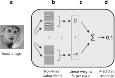
Figure 1: A Gabor-based encoding model for natural images. A cartoon depicting the encoding models that were used for the fMRI experiment (adapted from Kay et al.). In these models, natural images (a) are transformed into a vector of 10,409 features; features (b) measure the energy from two linear Gabor filters—tuned for specific spatial frequency, location in the image and orientation—with complementary phases. These features are combined according to a linear weight vector (c) that was fit separately for each voxel. The predicted response of a voxel for an image is the weighted sum of the features representing the image (d). The linear weights were fit on the training data consisting of responses to 1750 images.

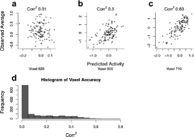
Figure 2: Prediction accuracy for V1 voxels. Predicted vs. observed average responses for three voxels in the V1 area, reflecting poor (a), medium (b) and high (c) prediction accuracies. Each point depicts the predicted response ($x$-axis) and the observed average response (across all repeats) for an image of the validation sample ($m=120$ images). (d) Histogram of prediction accuracy for all 1250 V1 voxels.

Data from the training sample was used to fit a quantitative receptive field model for each voxel, describing the fMRI response as a function of the input image. Here is a brief overview; more details on these V1 encoding models can be found in Vu et al. (2011). The model was based on multiple Gabor filters capturing spatial location, orientation and spatial-frequency of edges in the images (see Figure 1). Because of the tuning properties of the Gabor energy filters, this filter set is typically used for representing receptive fields of mammalian V1 neurons. Gabor filters ($d={}$10,409 filters) transformed each image into a feature vector in $\mathbb{R}^{d}$. For each of $Q$ voxels of interest, a linear weight vector relating the features to the measurements was estimated from the training data. Together, the transformation and linear weight vector result in a prediction rule that maps novel images to a real-valued response per voxel.

In their paper, Kay et al. measured prediction accuracy by comparing observations from the validation sample with the predicted responses for those images. The validation data consisted of a total of $T=1560$ measurements (per voxel): $m=120$ different images, each repeated $n=13$ times. Let $Y^{(r)}_{t}\in\mathbb{R}$ denote the measured fMRI activity at voxel $r$ and time $t$. Repeated measurements of the same image were averaged to reduce noise:

$$\bar{Y}{}^{(r)}_{j}=\mathop{\operatorname{avg}}_{t\dvtx h(t)=j}Y^{(r)}_{t},\qquad j=1,\ldots,m,$$

where $h(t)\in\{1,\ldots,m\}$ indexes the image that was shown at time $t$.

Let $f^{(r)}_{1},\ldots,f^{(r)}_{m}$ be the sequence of predictions for voxel $r$, and $\bar{f}{}^{(r)}$ their average. A single value per voxel summarizes prediction accuracy. That is,

$$\operatorname{Corr}^{2}\bigl{[}\bigl{(}f^{(r)}_{j}\bigr{)}_{j\leq m},\bigl{(}\bar{Y}{}^{(r)}_{j}\bigr{)}_{j\leq m}\bigr{]}:=\frac{(\sum_{j=1}^{m}(f^{(r)}_{j}-\bar{f}{}^{(r)})(\bar{Y}{}^{(r)}_{j}-\bar{Y}{}^{(r)}))^{2}}{\sum_{j=1}^{m}(f^{(r)}_{j}-\bar{f}{}^{(r)})^{2}\sum_{j=1}^{m}(\bar{Y}{}^{(r)}_{j}-\bar{Y}{}^{(r)})^{2}}.$$

In Figure 2 we show examples of voxels with low, intermediate and high prediction accuracies, and a histogram of the accuracy for all $1250$ voxels located within the V1 area. We can drop the superscript $r$ because each voxel is analyzed separately.

2.2 Correlation in the data

The goal of our work is to separate the two factors that determine the accuracy of prediction rules: the adequacy of the feature set or the linear model; and the noise level. Explainable variance represents the optimal accuracy if prediction were unrestricted by the choice of features and model.

We validate our explainable variance estimators by showing the estimators account well for the differences in prediction accuracy between $Q=1250$ voxels within the primary visual cortex (V1). This analysis depends on the assumption that the observed variation between voxels is primarily due to differences in the level of the signal-to-noise in the validation data, rather than, for example, differences in the adequacy of the feature set underlying the prediction models. Once the estimators are validated on this controlled setting, explainable variance can be used more broadly, for example, to compare the predictability levels of different functional areas.

Since we intend to use the validation data to estimate the explainable variance, we now give a few more details on how it was collected. Recall that the validation data consisted of $m=120$ images each repeated $n=13$ times [see Figure 3(a)]. These data were recorded in 10 separate sessions so that the subject could rest between sessions; the fMRI was recalibrated at the beginning of each session. Each session contained all presentations of 12 different images. A pseudo-random integer sequence ordered the repeats within a session.

When we measure correlation across many voxels, it appears that the design of the experiment induces strong correlation in the data. To see this, in Figure 3(b)–(d) we plot the correlation between measurements at different time slots (each time slot is represented by the vector of $Q=1250$ measurements). This plot shows qualitatively the correlation among individual voxels, including both noise driven and possibly stimuli-driven correlations. Clearly, there are strong correlations between time slots within a block, but no observable correlations between blocks. As these within-block correlation patterns do not correspond to the stimuli schedule, that is, randomized within a block, we conclude the correlations are largely due to noise. These noise correlations need to be taken into account to correctly estimate the explainable variance.

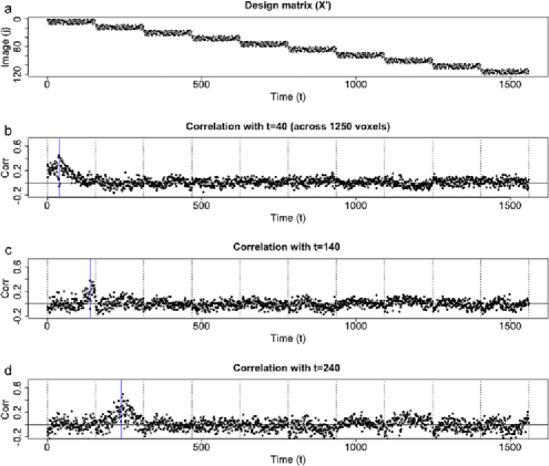
Figure 3: Data acquisition for the validation data. The responses in the validation set were collected in 10 separate sessions (blocks). Both the design matrix for the experiment and the noise correlation are influenced by this structure. In (a), the transposed design matrix $X^{\prime}$ is shown. This matrix records which image ($y$-axis) is displayed at each time slot $t$ ($x$-axis). Separate sets of 12 images were repeated $n=13$ times within each block, whereas no image was recorded in more than one block. In (b)–(d) temporal autocorrelation is displayed, as measured between a single time point [$t^{*}=40,140,240$ for (b), (c), (d), resp.] and all others points. The $t=t^{*}$ point is marked by a blue vertical line. On average, strong but nonsmooth correlations are found within the blocks, but separate blocks seem uncorrelated. Note that we calculate here the aggregate correlation of the voxels, but cannot use this same method to measure the autocorrelation of any specific voxel. Furthermore, the correlation depicted here is due to both noise and signal.

2.3 A probability model for the measurements

We introduce a probabilistic model for the measurements $\mathbf{Y}:=(Y_{t})_{t=1}^{T}$ at a single voxel. $\mathbf{Y}$ is modeled as a random effects model with additive, correlated noise [Williams (1952)]. We assume the observed response is the sum of two independent random processes: the signal process, which is random due to sampling of images into the validation set, and the noise process describing fluctuations unrelated to the stimuli. Additivity of noise is considered a good approximation for fMRI-event related designs and is commonly used [Buracas and Boynton (2002)]. The random effects model accounts for the generalization of prediction accuracy from the validation sample to the larger population of natural images.

2.3.1 Signal

Images are shown in a long sequence, in which each of the $m$ images in the random sample is repeated multiple times. The order of presentation is described by the design matrix $X\in\{0,1\}^{T\times m}$ (see Figure 3). Each row vector $X_{t}$ has a single 1 entry, which identifies the image shown at time $t$,

$$X_{t,j}=1\qquad\mbox{if the $j$th image in the sample is displayed at time $t$}.$$

For now, the sampling of images is conveyed through their effects on the measurement. We use a homogenous set of random variables [Owen (2007)] to represent the mean responses to the images in the sample. Let $A_{j}$ be the mean of the observed responses to the $j$th image in the sample. We assume that

$$A_{j}\sim\bigl{(}0,\sigma^{2}_{A}\bigr{)}\qquad\mbox{for }j=1,\ldots,m,$$

that is, $A_{j}$’s are i.i.d. with mean $0$ and variance $\sigma^{2}_{A}\geq 0$, but are not necessarily normally distributed. In the experiment we are analyzing, the randomness originates from sampling a large (infinite) population of images. We use $\mathbf{A}:=(A_{j})_{j=1}^{m}$ for the random-effect column vector, $\bar{A}:=\frac{1}{m}\sum_{j=1}^{m}A_{j}$ for the sample mean, and $s^{2}_{A}:=\frac{1}{(m-1)}\sum_{j=1}^{m}(A_{j}-\bar{A})^{2}$ for the sample variance of the random effects.

$X\mathbf{A}$ is the $T$-dimensional random signal vector, denoting the random effect at each measurement. To index the effect corresponding to time $t$, we use the shorthand $A_{(t)}:=X_{t}A$.

2.3.2 Noise

We assume the measurement noise process $\varepsilon=(\varepsilon_{t})_{t=1}^{T}$ is independent of the random signal vector $X\mathbf{A}$. We further assume the noise elements $\varepsilon_{t}$ have 0 mean, $\sigma^{2}_{\varepsilon}\geq 0$ variance, but may be autocorrelated. The unknown correlation, denoted by a matrix $\Sigma\in\mathbb{R}^{T\times T}(\operatorname{diag}(\Sigma)=\mathbf{1})$, captures the slow-changing hemodynamics of the BOLD and the effects of preprocessing on the BOLD signals. Hence,

$$\mathbb{E}_{\varepsilon}[\varepsilon_{t}]=0,\qquad\operatorname{cov}(\varepsilon_{t},\varepsilon_{u})=\sigma^{2}_{\varepsilon}\Sigma_{tu},\Sigma_{tt}=1,$$ (1)

or in matrix notation $\operatorname{cov}[\varepsilon]=\sigma^{2}_{\varepsilon}\Sigma$.

2.3.3 Model for observed responses

We are now ready to introduce the observed response (column) vector $\mathbf{Y}\in\mathbb{R}^{T}$ as follows:

$$\mathbf{Y}=X\mathbf{A}+\varepsilon$$ (2)

and for a single time slot $t$

$$Y_{t}=A_{(t)}+\varepsilon_{t}.$$

2.3.4 Response covariance

The model involves two independent sources of randomness: the image sampling, modeled by the random effects ($\mathbf{A}$), and the measurement noise $\varepsilon$. Assuming independence between $\mathbf{A}$ and $\varepsilon$, the covariance of $Y_{t}$ and $Y_{u}$ amounts to adding the individual covariances

$$\operatorname{cov}_{A,\varepsilon}(Y_{t},Y_{u}) = \operatorname{cov}_{A}(A_{(t)},A_{(u)})+\operatorname{cov}_{\varepsilon}(\varepsilon_{t},\varepsilon_{u})$$

$$= \sigma^{2}_{A}1_{(X_{t}=X_{u})}+\sigma^{2}_{\varepsilon}\Sigma_{tu}.$$

The first term on the RHS shows that treatment (random) effects are uncorrelated if they are based on different inputs, but are identical if based on the same input, with a variance of $\sigma_{A}^{2}$. In matrix form, we get

$$\mathbb{E}_{A,\varepsilon}[\mathbf{Y}]=0,\qquad\operatorname{cov}_{A,\varepsilon}(\mathbf{Y})=\sigma^{2}_{A}XX^{\prime}+\sigma^{2}_{\varepsilon}\Sigma.$$ (4)

2.4 Explainable variance and variance components

We are ready to define explainable variance, a scaled version of the treatment variance $\sigma^{2}_{A}$. Explainable variance is relevant to the performance of prediction models, a property we will discuss in Section 4.

Recall that $\bar{Y}_{j}$ are the averaged responses per image ($j=1,\ldots,m$ for the images in our sample), and let $\bar{Y}=\frac{1}{T}\sum_{t=1}^{T}Y_{t}$ be the global average response. Then the sample variance of averages is

$$\mathrm{MS}_{\mathrm{bet}}:=\frac{1}{m-1}\sum_{j=1}^{m}(\bar{Y}_{j}-\bar{Y})^{2}.$$ (5)

The notation $\mathrm{MS}_{\mathrm{bet}}$ refers to the mean-of-squares between treatments. Let us define the total variance $\bar{\sigma}{}^{2}_{Y}$ as the population mean of $\mathrm{MS}_{\mathrm{bet}}$,

$$\bar{\sigma}{}^{2}_{Y}:=\mathbb{E}_{A,\varepsilon}[\mathrm{MS}_{\mathrm{bet}}].$$ (6)

Note that $\bar{\sigma}{}^{2}_{Y}$ is not strictly the variance of any particular $\bar{Y}_{j}$; indeed, the variance of $\bar{Y}_{j}$ is not necessarily equal for different $j$’s. Nevertheless, we will loosely use the term variance here and later, owing to the parallels between these quantities and the variances in the i.i.d. noise case.

The average across repeats $\bar{Y}_{j}$ is composed of a signal part ($A_{j}$) and an average noise part ($\bar{\varepsilon}_{j}$); similarly, $\bar{Y}$ is composed of $\bar{A}$ and $\bar{\varepsilon}$. By partitioning the $\mathrm{MS}_{\mathrm{bet}}$, and taking expectations over the sampling and the noise, we get

$$\qquad\mathbb{E}_{A,\varepsilon}[\mathrm{MS}_{\mathrm{bet}}]=\mathbb{E}_{A}\Biggl{[}\frac{1}{m-1}\sum_{j=1}^{m}(A_{j}-\bar{A})^{2}\Biggr{]}+\mathbb{E}_{\varepsilon}\Biggl{[}\frac{1}{m-1}\sum_{j=1}^{m}(\bar{\varepsilon}_{j}-\bar{\varepsilon})^{2}\Biggr{]},$$ (7)

where the cross-terms cancel because of the independence of the noise from the sampling. We can call the expectation of the second term the noise level, or $\bar{\sigma}{}^{2}_{\varepsilon}$, and get the following decomposition:

$$\bar{\sigma}{}^{2}_{Y}=\sigma^{2}_{A}+\bar{\sigma}{}^{2}_{\varepsilon}.$$ (8)

In other words, the signal variance $\sigma^{2}_{A}$ and the noise level $\bar{\sigma}{}^{2}_{\varepsilon}$ are the signal and noise components of the total variance.

Finally, we define the proportion of explainable variance to be the ratio

$$\omega^{2}:=\sigma^{2}_{A}/\bar{\sigma}{}^{2}_{Y}.$$ (9)

Explainable variance measures the proportion of variance due to signal in the averaged responses; estimating it is the goal of this work. Note that by definition, $\omega^{2}$ is restricted to $[0,1]$.

To estimate $\omega^{2}$, we need estimators for $\bar{\sigma}{}^{2}_{Y}$ and $\sigma^{2}_{A}$. Whereas $\bar{\sigma}{}^{2}_{Y}$ can be directly estimated from the sample, to estimate $\sigma^{2}_{A}$ we need a method to separate the signal from the noise. In the following, we propose a method to distinguish them using their different covariance structures. We first develop some technical algebraic identities important for the estimation procedure. Some readers might prefer to skip directly to Section 3.

2.5 Quadratic contrasts

In this subsection we express $\mathrm{MS}_{\mathrm{bet}}$ as a quadratic contrast of the full data vector $\mathbf{Y}$. This contrast highlights the relation between $\bar{\sigma}{}^{2}_{Y}$ or $\bar{\sigma}{}^{2}_{\varepsilon}$ with both the design $XX^{\prime}$ and the measurement correlations $\Sigma$, and produces algebraic descriptions to be used for deriving the shuffle estimator. These are simple extensions of classical treatment of variance components [Townsend and Searle (1971)].

Denote $B:=XX^{\prime}/n$, the $\mathbb{R}^{T\times T}$ matrix in which

$$B_{tu}=\cases{\displaystyle\frac{1}{n},&\quad if $X_{t}=X_{u}$,\vspace*{4pt}\cr 0,&\quad otherwise,}$$ (10)

where $B$ is an averaging matrix, meaning that multiplication of a measurement vector by $B$ replaces each element in the vector by the treatment average, as in

$$(B\mathbf{Y})_{t}=\bar{Y}_{h(t)}.$$ (11)

It is easy to check that $B=B^{\prime}$ and $B=B^{2}$. Also, let $G\in\mathbb{R}^{T\times T},G_{tu}=1/T$ for $t,u=1,\ldots,T$, be the global average matrix, so that $(G\mathbf{Y})_{t}=\bar{Y},t=1,\ldots,T$. We can now express $\mathrm{MS}_{\mathrm{bet}}$ as a quadratic expression of $\mathbf{Y}$,

$$\mathrm{MS}_{\mathrm{bet}}=\frac{1}{(m-1)n}\bigl{\|}(B-G)\mathbf{Y}\bigr{\|}^{2},$$ (12)

or, more generally, as a quadratic function of any input vector,

$$\mathrm{MS}_{\mathrm{bet}}(\cdot):=\frac{1}{(m-1)n}\bigl{\|}(B-G)(\mathbf{\cdot})\bigr{\|}^{2}.$$ (13)

By replacing the $\mathrm{MS}_{\mathrm{bet}}$ with its quadratic form, a relation is exposed between the total variance, the design and the correlation of the noise:

$$\bar{\sigma}{}^{2}_{Y} = \mathbb{E}_{A,\varepsilon}\bigl{[}\mathrm{MS}_{\mathrm{bet}}(\mathbf{Y})\bigr{]}$$

$$= \frac{1}{(m-1)n}\mathbb{E}_{A,\varepsilon}\bigl{[}\operatorname{tr}\bigl{(}(B-G)\bigl{(}\mathbf{Y}^{\prime}\mathbf{Y}\bigr{)}(B-G)\bigr{)}\bigr{]}$$

$$= \frac{1}{(m-1)n}\operatorname{tr}\bigl{(}(B-G)\operatorname{cov}_{A,\varepsilon}(\mathbf{Y})\bigr{)}.$$

The signal effect and noise are additive, hence,

$$\frac{1}{(m-1)n}\operatorname{tr}\bigl{(}(B-G)\operatorname{cov}_{A}(\mathbf{Y})\bigr{)}+\frac{1}{(m-1)n}\operatorname{tr}\bigl{(}(B-G)\operatorname{cov}_{\varepsilon}(\mathbf{Y})\bigr{)}.$$

Substituting $\operatorname{cov}_{A}(\mathbf{Y})=n\sigma^{2}_{A}B$ and $\operatorname{cov}_{\varepsilon}(\mathbf{Y})=\sigma_{\varepsilon}^{2}\Sigma$,

$$\frac{1}{(m-1)n}\operatorname{tr}\bigl{(}(B-G)\bigl{(}n\sigma^{2}_{A}B\bigr{)}\bigr{)}+\frac{1}{(m-1)n}\operatorname{tr}\bigl{(}(B-G)\sigma_{\varepsilon}^{2}\Sigma\bigr{)}$$

$$\qquad=\frac{1}{(m-1)}\sigma^{2}_{A}\operatorname{tr}(B-G)+\frac{1}{(m-1)n}\sigma_{\varepsilon}^{2}\operatorname{tr}\bigl{(}(B-G)\Sigma\bigr{)}$$

$$\qquad=\sigma^{2}_{A}+\frac{1}{(m-1)n}\sigma_{\varepsilon}^{2}\operatorname{tr}\bigl{(}(B-G)\Sigma\bigr{)}.$$

Derivation 1

Under the model described in Section 2.3,

$$\bar{\sigma}{}^{2}_{Y}=\sigma^{2}_{A}+\frac{1}{(m-1)n}\sigma_{\varepsilon}^{2}\operatorname{tr}\bigl{(}(B-G)\Sigma\bigr{)}.$$ (14)

As a direct consequence of (8) and (14), we get an exact expression for the noise level

$$\bar{\sigma}{}^{2}_{\varepsilon}=\frac{1}{(m-1)n}\sigma_{\varepsilon}^{2}\operatorname{tr}\bigl{(}(B-G)\Sigma\bigr{)}.$$ (15)

This expression clarifies how $\bar{\sigma}{}^{2}_{\varepsilon}$ depends on the design, the noise variance and the noise autocorrelation. As expected, $\bar{\sigma}{}^{2}_{\varepsilon}$ scales linearly with the noise variance of the individual measurements $\sigma^{2}_{\varepsilon}$. More interesting is that $\bar{\sigma}{}^{2}_{\varepsilon}$ depends linearly on $\operatorname{tr}(B\Sigma)$—the interplay between the design and the noise autocorrelation.

Note that if the within treatment noise is uncorrelated, this expression simplifies to a classical ANOVA result. Uncorrelated noise within treatments manifests, in a properly sorted version of $\Sigma$, as small $n\times n$ identity blocks. Therefore, $\operatorname{tr}((B-G)\Sigma)=(m-1)\sigma^{2}_{\varepsilon}$ and $\bar{\sigma}{}^{2}_{\varepsilon}=\sigma^{2}_{\varepsilon}/n$. In that case $\bar{\sigma}{}^{2}_{Y}=\sigma^{2}_{A}+\sigma^{2}_{\varepsilon}/n$, and by plugging in an estimator of $\sigma^{2}_{\varepsilon}$, we can directly estimate $\bar{\sigma}{}^{2}_{\varepsilon}$ and $\sigma^{2}_{A}$. The estimator for $\omega^{2}$ is

$$\hat{\omega}{}^{2}=1-\frac{1}{F}$$

with $F$ being the standard $F$ statistic. This is the method-of-moments estimator described fully in Section 6.1.

On the other hand, when some correlations within repeats are greater than 0, $\sigma^{2}_{\varepsilon}/n$ underestimates the noise level and inflates the explainable variance. In the next section we introduce the shuffle estimators which can deal with correlated noise.

3 Shuffle estimators for signal and noise variances

In this section we propose new estimators called the shuffle estimators for the signal and noise levels, and for the explainable variance. As in (8), $\bar{\sigma}{}^{2}_{Y}=\sigma^{2}_{A}+\bar{\sigma}{}^{2}_{\varepsilon}$, but the noise level $\bar{\sigma}{}^{2}_{\varepsilon}$ is a function of the (unknown) measurement correlation matrix $\Sigma$. Using shuffle estimators, we can estimate $\sigma^{2}_{A}$ and $\bar{\sigma}{}^{2}_{\varepsilon}$ without having to estimate the full $\Sigma$ or imposing unrealistically strong conditions on it.

The key idea is to artificially create a second data vector that will have similar noise patterns as our original data (see Figure 4). We do this by permuting, or shuffling, the original data along symmetries that we identify in the data collection. In Section 3.1 we formalize the definition of such permutations that conserve the noise correlation, and give plausible examples for neuroscience measurements. In Section 3.2 we compare the variance of averages ($\mathrm{MS}_{\mathrm{bet}}$) of the original data [Figure 4(b)], with the same contrast computed on the shuffled data (c). Because repeated measures for the same image are shuffled into different categories, the variance due to signal will be reduced in the shuffled data. We derive an unbiased estimator for signal variance $\sigma^{2}_{A}$ based on this reduction in variance, and use the plug-in estimators to estimate $\bar{\sigma}{}^{2}_{\varepsilon}$ and $\omega^{2}$.

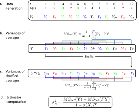
Figure 4: Cartoon of the shuffle estimator. (a) Data is generated according to a predetermined design, with each color representing repeats of a different image. (b) Repeats of each image are averaged together and the sample variance is computed on these averages. (c) Data is shuffled by $P$, in this example reversing the order. Now measurements which do not originate from the same repeat are averaged together ($\bar{Y}{}^{*}_{j}$’s), and the sample variance of the new averages is computed. These averages should have a lower variance in expectation, and we can calculate the reduction amount $\alpha=\frac{1}{m-1}\operatorname{tr}((B-G)PBP^{\prime})$, where $B=XX^{\prime}/n$. (d) The shuffle estimator for signal variance is the difference between the two sample variances, after correction of $1-\alpha$.

3.1 Noise-conserving permutation for $\mathbf{Y}$ with respect to design $X$

A prerequisite for the shuffle estimator is to find a permutation that will conserve the noise contribution to $\bar{\sigma}{}^{2}_{Y}$. We will call such permutations noise-conserving w.r.t. to $X$.

Recall (15),

$$\bar{\sigma}{}^{2}_{\varepsilon}=\frac{1}{(m-1)n}\operatorname{tr}\bigl{(}(B-G)\bigl{(}\sigma^{2}_{\varepsilon}\Sigma\bigr{)}\bigr{)},$$

where $\sigma^{2}_{\varepsilon}\Sigma=\operatorname{cov}_{\varepsilon}[\mathbf{Y}]$ as before. Let $P\in\mathbb{R}^{T\times T}$ be a permutation matrix. Then we have the following:

Definition 1.

$P$ is noise conserving w.r.t. $X$, if

$$\operatorname{tr}\bigl{(}(B-G)P\sigma^{2}_{\varepsilon}\Sigma P^{\prime}\bigr{)}=\operatorname{tr}\bigl{(}(B-G)\sigma^{2}_{\varepsilon}\Sigma\bigr{)}.$$ (16)

Equivalently,

$$\operatorname{tr}\bigl{(}(B-G)\operatorname{cov}_{\varepsilon}[P\cdot\mathbf{Y}]\bigr{)}=\operatorname{tr}\bigl{(}(B-G)\operatorname{cov}_{\varepsilon}[\mathbf{Y}]\bigr{)}.$$

Although we define the noise-conserving property based on the covariance, replacing the covariance with the correlation matrix $\Sigma$ would not change the class of noise-conserving permutations.

We consider first two important cases of noise conservation. Though most useful noise-conserving permutations will be derived from assumptions regarding the noise correlation $\Sigma$, the noise-conservation property can be derived from the design $X$ as well. This can be seen in the first example.

3.1.1 Trivial noise-conserving permutations

A permutation $P$ that simply relabels the treatments is not a desirable permutation, even though it is noise conserving. We call such permutations trivial:

Definition 2.

A permutation $P$, associated with permutation function $g_{P}\dvtx\{1,\ldots,T\}\rightarrow\{1,\ldots,T\}$, is trivial if

$$X_{t}=X_{u}\quad\Rightarrow\quad X_{g_{P}(t)}=X_{g_{P}(u)}\qquad\forall t,u.$$ (17)

It is easy to show that a trivial $P$ does nothing, that is, $\mathrm{MS}_{\mathrm{bet}}(P\mathbf{Y})=\mathrm{MS}_{\mathrm{bet}}(\mathbf{Y})$.

3.1.2 Noise-conserving permutations based on symmetries of $\Sigma$

A useful class of nontrivial noise-conserving permutations is the class of symmetries in the correlation matrix $\Sigma$: a symmetry of $\Sigma$ is a permutation $P$ such that $P\Sigma P^{\prime}=\Sigma$. If $P$ is a symmetry of $\Sigma$, then $P$ is noise conserving regardless of the design. Here are three important general classes of symmetries which are commonly applicable in neuroscience:

1. [3.]

2. Uncorrelated noise. The obvious example is the uncorrelated noise case $\Sigma=I$ where all responses are exchangeable. Hence, any permutation is noise conserving.

3. Stationary time series. Neuroscience data typically are recorded in a long sequence containing a large number of serial recordings at constant rates. It is natural to assume that correlations between measurements will depend on the time passed between the two measures, rather than on the location of the pair within the sequence. We call this the stationary time series. Under this model $\Sigma$ is a Toeplitz matrix parameterized by $\{\rho_{d}\}_{d=0}^{T-1}$, the set of correlation values $\Sigma_{t,u}=\rho_{d}$, where $d=|t-u|$. Though the correlation values $\rho_{d}$’s are related, this parameterization does not enforce any structure on them. This robustness is important in the fMRI data we analyze. For this model, a permutation that reverses the measurement vector is noise conserving

   $$(P\mathbf{Y})_{t}=\mathbf{Y}_{T+1-t}.$$

   This is the permutation we use on our data in Section 6.

   The shift operators of the form $(P\mathbf{Y})_{t}=(\mathbf{Y})_{t+k}$ define a transformation that, up to edge effects, can be considered noise conserving.

4. Block effect models. Another important case is when measurements are collected in distinct sessions or blocks. Measurements from different blocks are assumed independent, but measurements within the same block may be correlated, perhaps because of calibration of the measurement equipment. We index the block assignment of time $t$ with $\beta(t)$. A simple parameterization for noise correlation would be to let $\Sigma_{t,u}=\zeta(\beta(t),\beta(u))$ depend only on the block identity of measurements $t$ and $u$. We call this the block structure. Under the block structure, any permutation $P$ (associated with function $g_{P}$) that maintains the identity of blocks, meaning

   $$\beta(t)=\beta(u)\quad\Rightarrow\quad\beta\bigl{(}g_{P}(t)\bigr{)}=\beta\bigl{(}g_{P}(u)\bigr{)},$$ (18)

   would be noise conserving w.r.t. any $X$.

The scientist is given much freedom in choosing the permutation $P$, and should consider both the variance of the estimator and the estimator’s robustness against plausible noise-correlation structures. Establishing criteria for choosing the permutation $P$ is the topic of current research.

3.2 Shuffle estimators

We can now state the main results. From the following lemma we observe that every noise-conserving permutation establishes a linear mean equation with two parameters: $\sigma^{2}_{A}$ and $\bar{\sigma}{}^{2}_{\varepsilon}$. The coefficient of $\bar{\sigma}{}^{2}_{\varepsilon}$ is 1, whereas the coefficient for $\sigma^{2}_{A}$ is the constant

$$\alpha=\alpha(X,P)=\frac{1}{m-1}\operatorname{tr}\bigl{(}(B-G)\bigl{(}PBP^{\prime}\bigr{)}\bigr{)},$$ (19)

which depends only on the design $B=XX^{\prime}/n$ and the permutation $P$—both known to the scientist. The size of $\alpha$ reflects how well P mixes the treatments; the greater the mix, the smaller $\alpha$.

Lemma 1

If $P$ is a noise-conserving permutation for $\mathbf{Y}$, then [(a)]

$\mathbb{E}_{A,\varepsilon}[\mathrm{MS}_{\mathrm{bet}}(P\mathbf{Y})]=\alpha\sigma^{2}_{A}+\bar{\sigma}{}^{2}_{\varepsilon}$,

$\alpha\leq 1$, and the inequality is strict iff $P$ is nontrivial.

The proof of (a) involves derivations as in Section 2.5 [e.g., equation (14)], and the proof of (b) further requires the Cauchy–Schwarz inequality. Both are found in the supplementary materials [Benjamini and Yu (2013)].

The consequence of part (b) is that for any nontrivial $P$, we get a second mean equation, which is linearly independent from the equation based on the original data (because $\alpha<1$). In other words, for a nontrivial $P$, the equation set

$$\cases{\mathbb{E}_{A,\varepsilon}\bigl{[}\mathrm{MS}_{\mathrm{bet}}(\mathbf{Y})\bigr{]}=\sigma^{2}_{A}+\bar{\sigma}{}^{2}_{\varepsilon},\vspace*{2pt}\cr\mathbb{E}_{A,\varepsilon}\bigl{[}\mathrm{MS}_{\mathrm{bet}}(P\mathbf{Y})\bigr{]}=\alpha\sigma^{2}_{A}+\bar{\sigma}{}^{2}_{\varepsilon}}$$ (20)

has a unique solution. Solving the two equations above, we arrive at an unbiased estimator for the signal variance.

Definition 3.

The shuffle estimator for the signal variance is defined as

$$\hat{\sigma}{}^{2}_{A}=\frac{\mathrm{MS}_{\mathrm{bet}}(\mathbf{Y})-\mathrm{MS}_{\mathrm{bet}}(P\mathbf{Y})}{1-\alpha}.$$ (21)

Finally, we can plug in $\hat{\sigma}{}^{2}_{A}$ and $\hat{\bar{\sigma}}{}^{2}_{Y}=\mathrm{MS}_{\mathrm{bet}}(\mathbf{Y})$ to get the shuffle estimator for the explainable variance $\omega^{2}$:

$$\hat{\omega}{}^{2}=\frac{\hat{\sigma}{}^{2}_{A}}{\mathrm{MS}_{\mathrm{bet}}(\mathbf{Y})}=\frac{1}{1-\alpha}\biggl{(}1-\frac{\mathrm{MS}_{\mathrm{bet}}(P\mathbf{Y})}{\mathrm{MS}_{\mathrm{bet}}(\mathbf{Y})}\biggr{)}.$$

1. [3.]

2. An unbiased estimator of the noise level $\bar{\sigma}{}^{2}_{\varepsilon}$ can be derived from equations (21) and (8),

   $$\hat{\bar{\sigma}}{}^{2}_{\varepsilon}=\mathrm{MS}_{\mathrm{bet}}-\hat{\sigma}{}^{2}_{A}.$$

3. Because $\hat{\sigma}{}^{2}_{A}$ estimates a nonnegative quantity, it is preferable to restrict $\hat{\sigma}{}^{2}_{A}$ to nonnegative values by taking $\hat{\sigma}{}^{2}_{A+}=\max\{0,\hat{\sigma}{}^{2}_{A}\}$.

4. The estimator is consistent under proper decay of the dependance. This statement is conditional on the asymptotic setup: explainable variance typically changes as the number of measurements ($T$) increases. Nevertheless, the shuffle estimator is consistent for a sequence of data sets (indexed by $k=1,2,\ldots$) of growing sizes $[T(k)\to\infty]$ for which total variance and explainable variance converge if (a) the number of treatments $m(k)$ grows to $\infty$ and (b) the dependence decays. For $\mathbf{Y}$ distributed as a multivariate gaussian, a sufficient condition for (b) can be given in terms of eigenvalues of $\Sigma$:

5. The largest $m-1$ eigenvalues $\lambda_{(1)}(k),\ldots,\lambda_{(m-1)}(k)$ of the noise correlation matrix $\Sigma(k)$ satisfy

   $$\frac{1}{n^{2}(m-1)^{2}}\sum_{i=1}^{m-1}\lambda_{(i)}^{2}(k)\to 0\qquad\mbox{as }k\to\infty.$$

   Conditions (a) and (b*) assure that $\operatorname{var}(\mathrm{MS}_{\mathrm{bet}}(\mathbf{Y}_{k}))\to 0$ as $k\to\infty$. The proof relies mainly on the expression for the variance of a quadratic contrasts, as found, for example, in Searle (1971). For the proof of these results refer to the supplementary materials [Benjamini and Yu (2013)].

4 Evaluating prediction for correlated responses

Although there are many uses for estimating the explainable variance, we focus on its role in assessing prediction models. Roddey, Girish and Miller (2000) show that explainable variance upper bounds the accuracy of prediction on the sample when noise is i.i.d. We generalize their results for arbitrary noise correlation and account for generalization from sample to population. As shown in Lemma 2, the noise level $\bar{\sigma}{}^{2}_{\varepsilon}$ is the optimal expected loss under mean square prediction error (MSPE) loss, and the explainable variance $\omega^{2}$ approximates the accuracy under squared-correlation $\operatorname{Corr}^{2}$ utility.

A more explicit notation setup is needed for studying the relation between predictions and signal responses. Let $f$ be a prediction function that predicts a real-valued response to any possible image $I$, out of a large population of $M$ images,

$$f\dvtx\{I_{i}\}_{i=1}^{M}\to\mathbb{R}.$$ (22)

We will assume $f$ does not depend on the sample we are evaluating, meaning that it was fit on separate data. We usually think of $f$ as using some aspects of the image to predict the response, although we do not restrict it in any parametric way to the image.

Prediction accuracy is measured only on the $m$ images sampled for the (nonoverlapping) validation set. Let $\mathbf{s}\dvtx\{1,\ldots,m\}\to\{1,\ldots,M\}$ be the random sampling function, and $I_{\mathbf{s}(j)}$ the random image chosen for the $j$th sample image.

Furthermore, let us introduce notation relating the random effects to the image sampling. For this, assume each image is associated with a mean activation quantity $\mu_{i}$, so that $\sum\mu_{i}=0$ and $\sum\mu_{i}^{2}=\sigma^{2}_{A}$. Then the random effects $A_{j}$ defined before can now be described $A_{j}=\mu_{\mathbf{s}(j)}$.

To evaluate prediction accuracy, the predicted response $f(I_{\mathbf{s}(j)})$ is compared with the averaged (observed) response for that image $\bar{Y}_{j}$. We consider two common accuracy measures: mean squared prediction error ($\mathrm{MSPE}[f]$) and the squared correlation ($\operatorname{Corr}^{2}[f]$), defined

$$\mathrm{MSPE}[f] := \frac{1}{m-1}\sum_{j=1}^{m}\bigl{(}f(I_{\mathbf{s}(j)})-\bar{Y}_{j}\bigr{)}^{2},$$ (23)

$$\operatorname{Corr}^{2}[f] := \operatorname{Corr}_{j}^{2}\bigl{(}f(I_{\mathbf{s}(j)}),\bar{Y}_{j}\bigr{)}$$

$$= \frac{(1/(m-1)\sum_{j=1}^{m}(f(I_{\mathbf{s}(j)})-\bar{f}_{\mathbf{s}})(\bar{Y_{j}}-\bar{Y}))^{2}}{1/(m-1)\sum_{j=1}^{m}(f(I_{\mathbf{s}(j)})-\bar{f}_{\mathbf{s}})^{2}\sum_{j=1}^{m}(\bar{Y_{j}}-\bar{Y})^{2}},$$

where $\bar{f_{\mathbf{s}}}$ denotes the average of the predictions for the sample.

We will state and discuss the results relating the explainable variance to optimal prediction; the proof can be found in the supplementary materials [Benjamini and Yu (2013)].

Lemma 2

Let $f^{*}\dvtx\{I_{i}\}_{i=1}^{M}\to\mathbb{R}$ be the prediction function that assigns for each stimulus $I_{i}$ its mean effect $\mu_{i}$, or $f^{*}(I_{i})=\mu_{i}$. Under the model described in Section 2.3, [(a)]

$f^{*}=\arg\min_{f}\mathbb{E}_{A,\varepsilon}$ $[\mathrm{MSPE}[f]]$;

$\bar{\sigma}{}^{2}_{\varepsilon}=\mathbb{E}_{A,\varepsilon}$ $[\mathrm{MSPE}[f^{*}]]$ $({=}\min_{f}\mathbb{E}_{A,\varepsilon}$ $[\mathrm{MSPE}[f]]$ by (a));

$\omega^{2}\approx\mathbb{E}_{A,\varepsilon}[\operatorname{Corr}^{2}[f^{*}]]$ with a bias term smaller than $\frac{1}{m-1}$.

Under our random effects model, the best prediction (in MSPE) is obtained by the mean effects, or $f^{*}$. More important to us, the accuracy measures associated with the optimal prediction $f^{*}$ can be approximated by signal and noise levels: $\bar{\sigma}{}^{2}_{\varepsilon}$ for $\mathrm{MSPE}[f^{*}]$ and $\omega^{2}$ for $\operatorname{Corr}^{2}[f^{*}]$.

The main consequence of this lemma is that the researcher does not need a “good” prediction function to estimate the “predictability” of the response. Prediction is upper-bounded by $\omega^{2}$, a quantity which can be estimated without setting a specific function in mind. Moreover, when a researcher does want to evaluate a particular prediction function $f$, $\hat{\omega}{}^{2}$ can serve as a yardstick with which $f$ can be compared. If $\operatorname{Corr}^{2}[f]\approx\hat{\omega}{}^{2}$, the prediction error is mostly because of variability in the measurement. Then the best way to improve prediction is to reduce the noise by preprocessing or by increasing the number of repeats. On the other hand, if $\operatorname{Corr}^{2}[f]\ll\hat{\omega}{}^{2}$, there is still room for improvement of the prediction function $f$.

5 Simulation

We simulate data with a noise component generated from either a block structure or a times-series structure, and compute shuffle estimates for signal variance and for explainable variance. For a wide range of signal-to-noise regimes, our method produces unbiased estimators of $\sigma^{2}_{A}$. These estimators are fairly accurate for sample sizes resembling our image-fMRI data, and the bias in the explainable variance $\omega^{2}$ is small compared to the inherent variability. These results are shown in Figure 5. In Figure 6 we show that under nonzero $\sigma^{2}_{A}$, the shuffle estimates have less bias and lower spread compared to the parametric model using the correctly specified noise correlation.

Figure 5: Simulations for the block and time-series. (a) Simulation results comparing shuffle estimates for signal variance $\sigma^{2}_{A}$ (black) and explainable variance $\omega^{2}$ (blue) to the true population values (dashed line). Noise correlation followed an independent block structure: noise within blocks was correlated, and between blocks was independent. The $x$-axis represents the true signal variance $\sigma^{2}_{A}$ of the data, and the $y$-axis marks the average of the estimates and $[0.25,0.75]$ quantile range. (b) A similar plot for data generated under a stationary time-series model.

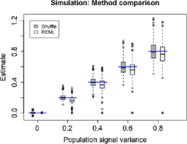
Figure 6: Comparison of methods on simulation. Each pair of box-plots represents the estimated signal variance $\sigma^{2}_{A}$ using the shuffle estimator (dark gray) and REML (light gray) for 1000 simulations. The blue horizontal line represents the true value of $\sigma^{2}_{A}$. The REML estimator assumes the correct model for the noise, while the shuffle estimator only assumes a stationary time series. When there is no signal, REML outperforms the shuffle estimators, but in all other cases it is both biased and has greater spread.

5.1 Block structure

For the block structure we assumed the noise is composed of an additive random block effect constant within blocks ($b_{k}$, $k=1,\ldots,B$ blocks), and an i.i.d. Gaussian term ($e_{t}$, $t=1,\ldots,T$)

$$Y_{t}=A_{(t)}+b_{\beta(t)}+e_{t}.$$

$A_{j},b_{k}$ and $e_{t}$ are sampled from centered normal distributions with variances ($\sigma^{2}_{A},\sigma^{2}_{b},\sigma^{2}_{e}$). We used $\sigma^{2}_{b}=0.5,\sigma^{2}_{e}=0.7$, and varied the signal level $\sigma^{2}_{A}=0,0.1,\ldots,0.9$. We used $m=120$, $n=15$, with all presentations of every 5 stimuli composing a block ($B=20$ blocks). For each of these scenarios we ran 1000 simulations, sampling the signal, block and error effects. $\mathrm{MS}_{\mathrm{bet}}$ was estimated the usual way, and $P$ was chosen to be a random permutation within each block ($\alpha=0.115$). The results are shown in Figure 5(a).

5.2 Time-series model

For the time-series model we assumed the noise vector $e\in\mathbb{R}^{T}$ is distributed as a multivariate Gaussian with mean 0 and a covariance matrix $\Sigma$, where $\Sigma$ is an exponentially decaying covariance with a nugget,

$$\Sigma_{tu}=\rho_{|t-u|}=\lambda_{1}\cdot\exp\bigl{\{}-|t-u|/\lambda_{2}\bigr{\}}+(1-\lambda_{1})1_{(t=u)}.$$

Then $Y=A_{(t)}+e_{t}$ with the random effects $A_{(t)}$ sampled from $\mathcal{N}(0,\sigma^{2}_{A})$ for $\sigma^{2}_{A}=0,0.1,\ldots,0.9$. We used $m=120,n=15$, and the parameters for the noise were $\lambda_{1}=0.7$ and $\lambda_{2}=30$, meaning $\rho_{125}\approx 0.01$. The schedule of treatments was generated randomly. For each of these scenarios we ran 1000 simulations, sampling the signal and the noise. In Figure 5(b) we estimated the shuffle estimator with $P$ the reverse permutation ($g_{P}(t)=T+1-t$), resulting in $\alpha=0.064$.

5.3 Comparison to REML

In Figure 6 we used time-series data to compare $\sigma^{2}_{A}$ estimates based on the shuffle estimators to those obtained by an REML estimator with the correct parametrization for the noise correlation matrix. We used the nlme package in R to fit a repeated measure analysis of variance for the exponentially decaying correlation of noise with a nugget effect. The comparison included 1000 simulations for $\sigma^{2}_{A}=0,0.2,0.4,0.6,0.8$ and a noise model identical to Section 5.2.

5.4 Results

Figure 5 describes the performance of shuffle estimates on two different scenarios: block correlated noise (a), and stationary time-series noise (b). For signal variance (black) the shuffle estimator gives unbiased estimates. The shuffle estimator for explainable variance is not unbiased, but the bias is negligible compared to the variability in the estimates. In Figure 6 we compare the signal variance estimates based on the shuffle estimator (dark gray) with estimates based on REML (light gray). The estimates based on the shuffle have no bias, while those based on REML underestimate the signal. The variance of the REML estimates is slightly larger, due in part to rare events (between 1%–0.5% of runs) in which the estimated signal variance was effectively 0—perhaps indicating a problem with the optimization.

6 Data

We are now ready to evaluate prediction models using the shuffle estimates for explainable variance. Prediction accuracy was measured for encoding models of 1250 voxels within the primary visual cortex (V1). Because V1 is functionally homogenous, encoding models for voxels within this cortical area should work similarly. As observed in Figure 2, there is large variation between prediction accuracies for the different voxels. We try to explain this observed variation as a result of variation in the explainable variance. To do this, prediction accuracy values for these 1250 voxels are compared to the explainable variance estimates generated by the shuffle estimator for each voxel. We also compare the accuracy values to alternative estimates for explainable variance, using the method of moments for uncorrelated noise, and REML under several parameterizations for the noise.

6.1 Methods

We estimate the explainable variance of voxels ($\omega^{2}=\break\sigma^{2}_{A}/\bar{\sigma}{}^{2}_{Y}$) with several different methods. The methods differ in how $\sigma^{2}_{A}$ is estimated; all methods use the sample averages variance $\mathrm{MS}_{\mathrm{bet}}(\mathbf{Y})$ for $\bar{\sigma}{}^{2}_{Y}$ and plug in the two estimates into $\omega^{2}$. We estimate $\omega^{2}$ separately for each voxel ($r=1,\ldots,1250$). The methods we compare are as follows:

1. [3.]

2. The shuffle estimator. We assume the noise follows a stationary time-series model within each block and is independent between the blocks. We therefore choose a permutation $P$ that reverses the order of the measurements, $(P\mathbf{Y})_{t}=\mathbf{Y}_{T+1-t}$. Because the size of the blocks is identical, reversing the order of the data vector is equivalent to reversing the order within each block, $\alpha=0.14$. Specifically, the estimator is restricted to be positive:

   $$\hat{\sigma}{}^{2}_{A+}=\max\biggl{\{}\frac{\mathrm{MS}_{\mathrm{bet}}(\mathbf{Y})-\mathrm{MS}_{\mathrm{bet}}(P\mathbf{Y})}{1-\alpha},0\biggr{\}}$$

   for signal variance, and $\hat{\omega}{}^{2}=\hat{\sigma}{}^{2}_{A+}/\mathrm{MS}_{\mathrm{bet}}$ for the explainable variance.

3. An estimator ($\tilde{\omega}{}^{2}$) unadjusted for correlation. We use the mean square within ($\mathrm{MS}_{\mathrm{wit}}=\frac{1}{(m-1)n}\sum_{j=1}^{m}\sum_{t\dvtx h(t)=j}(Y_{t}-\bar{Y}_{j})^{2}$) contrast to estimate the noise variance $\sigma^{2}_{\varepsilon}$, scale by $1/n$ to estimate the noise level $\bar{\sigma}{}^{2}_{\varepsilon}$, and remove the scaled estimate from $\mathrm{MS}_{\mathrm{bet}}$,

   $$\tilde{\sigma}{}^{2}_{A}=\mathrm{MS}_{\mathrm{bet}}-\mathrm{MS}_{\mathrm{wit}}/n.$$

   Explainable variance is obtained by plug-in estimator $\tilde{\omega}{}^{2}=\tilde{\sigma}{}^{2}_{A}/\mathrm{MS}_{\mathrm{bet}}$.

4. Estimators based on a parametric noise model.

   • We assume the noise is generated from an exponentially decaying correlation matrix, with a nugget effect. This means

     $$\Sigma_{t,t+d}=\lambda_{2}\exp(-d/\lambda_{1})+1_{(d=0)}(1-\lambda_{2}),$$

     where the rate of decay $\lambda_{1}$ and nugget effect $\lambda_{2}$ were additional parameters. If $\lambda_{2}=0$, this is equivalent to the $\operatorname{AR}(1)$ model.

   • Alternatively, we assume the noise is generated from an $\operatorname{AR}(3)$ process or $\varepsilon_{t}=\eta_{t}+\sum_{k=1}^{3}a_{k}\varepsilon_{t-k}$. This models allows for nonmonotone correlations.

   We use the nlme package in R to estimate the signal variance of this model using restricted maximum likelihood [REML, e.g., Laird, Lange and Stram (1987)], and use the plug-in estimator for the explainable variance.

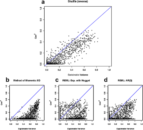
Figure 7: Optimal vs. observed prediction accuracy. The estimated optimal prediction is compared with observed prediction ($\operatorname{Corr}^{2}$), each point representing a V1 response. The optimal prediction estimated by (a) shuffle estimators accounting for stationary noise distributions; (b) Method of moments estimator assuming independent noise; (c) REML estimator assuming exponential decay of noise with nugget within blocks; and (d) REML estimator assuming an $\operatorname{AR}(3)$ model for the noise correlation within blocks. The $x=y$ is plotted in blue.

6.2 Results

In Figure 7 we compare the prediction accuracy of the voxels to estimates of the explainable variance. Each panel has 1250 points representing the 1250 voxels: the $x$ coordinate is the estimate of explainable variance for the voxel, and the $y$ coordinate is $\operatorname{Corr}^{2}[f]$ for the Gabor-based prediction rule. The large panel shows the shuffle estimators for explainable variance. The relation between $y=\operatorname{Corr}^{2}[f]$ and $\hat{\omega}{}^{2}$ is very linear ($r=0.9$). The estimated slope and intercepts (using least squares) for this relation are $y\approx 0.66\cdot\hat{\omega}^{2}-0.009$. Note that almost all voxels for which accuracy is close to random guessing ($\operatorname{Corr}^{2}[f]<0.05$) could be identified based on low explainable variance without knowledge of the specific feature set.

When we try to repeat this analysis with other $\omega^{2}$ estimators, explainable variance estimates are no longer strongly related with the prediction accuracy. When correlation in the noise is ignored (b), signal strength is greatly overestimated. In particular, some of the voxels for which prediction accuracy is almost 0 have very high estimates of explainable variance (as high as $\tilde{\omega}{}^{2}=0.8$). In contrast to the shuffle estimates, it is hard to learn from these explainable variance estimates about the prediction accuracy for a voxel.

This incompatibility of prediction accuracy and explainable variance estimates is also observed when the estimates are based on maximum likelihood methods that parameterize the noise matrix. For the $\operatorname{AR}(3)$ model in (d), we see variability between explainable variance estimates for voxels with given prediction accuracy level. The smaller model (c) seems to suffer from both overestimation of signal and from high variance.

7 Discussion

We have presented the shuffle estimator, a resampling-based estimator for the explainable variance in a random-effects additive model with autocorrelated noise. Rather than parameterize and estimate the correlation matrix of the noise, the shuffle estimator treats the contribution of the noise to the total variance as a single parameter. Symmetries in the data collection process indicate those permutations which, when applied to the original data, would not change the contribution of the noise. An unbiased estimator of the signal variance is derived from differences between the total variance of the original data vector and the shuffled vector. The resulting estimate of signal variance is plugged in as the enumerator for the explainable variance ratio estimate.

For a brain-encoding experiment, we have shown that the strong correlation present in the fMRI measurements greatly compromises classical methods for estimating explainable variance. We used prediction accuracy measures of a well-established parametric model for voxels in the primary visual cortex as correlates of signal variance at each of the voxels. Shuffle estimates explained most of the variation in prediction accuracy between voxels, even though they were blind to features of the image. Other methods did not do well: methods that ignored noise correlation seem to greatly overestimate the explainable variance, while methods that estimated the full correlation matrix were considerably less informative with regards to prediction accuracy. We consider this convincing evidence that the shuffle estimators for explainable variance can be used reliably even when no gold-standard prediction model is present.

Explainable variance is an assumption-less measure of signal, in that it makes no assumptions about the structure of the mean function that relates the input image to response. We find it attractive that the shuffle estimator for explainable variance similarly requires only weak assumptions for the correlation of the noise. This makes the shuffle estimator a robust tool, which can be used at different stages of the processing of an experiment: from optimizing of the experimental protocol, through choosing the feature space for the prediction models, to fitting the prediction models.

Choice of permutations

The bias and variance of the shuffle estimator depend on the permutation underlying the shuffle. Different permutations pose different assumptions on the noise correlation as well as provide a different mix of treatments corresponding to different $\alpha$s. We recommend the permutation be chosen prior to the analysis, based on the expected noise structure and the mixing constants ($\alpha$s), to minimize the risk of data snooping. Optimally, the experiment could be designed so that a specific permutation—perhaps the reverse permutation—will mix treatments well, resulting in a low $\alpha$. In our experiment, the reverse and other regular permutations such as shifts had low $\alpha$s because the design was generated using an irregular pseudo-random sequence. Moreover, when several noise-conserving permutations exist and have similar $\alpha$s, it may be preferable to average the corresponding shuffle estimators to reduce the variance of the estimators.

In cases were no symmetry permutations are useable, a wider class of “almost noise-conserving” permutations can be considered. To give concrete examples, consider the following two permutations: A cyclic left-shift permutation so that $(P_{1}\mathbf{Y})_{t}=\mathbf{Y}_{t+1}$ for $t=1,\ldots,T-1$, and $(P_{1}\mathbf{Y})_{T}=\mathbf{Y}_{1}$; and a permutation of odd and even channels $(P_{2}\mathbf{Y})_{2s-1}=\mathbf{Y}_{2s}$, $(P_{2}\mathbf{Y})_{2s}=\mathbf{Y}_{2s-1}$, for $s=1,\ldots,T/2$. Neither is an exact symmetry of a covariance matrix that represents a stationary time series. In $P_{1}$, the first measurement in each block is not correlated to the sequence. $P_{2}$ is even farther from symmetry, in that the medium and long-range correlations are conserved but the local structure is scrambled.

Nevertheless, the shuffle estimates from either $P_{1}$ or $P_{2}$ produce, when compared to predictions, population results that are similar to those observed for the reverse permutation. The new estimates compare in both linearity, with $r=0.905$ between $\operatorname{Corr}^{2}[f^{*}]$ and $\hat{\omega}{}^{2}$ for both $P_{1}$ and $P_{2}$ compared to $r=0.9$ for the reverse permutation, as well in the slope (0.65 for $P_{1}$, 0.68 for $P_{2}$) of the linear trend and its intercept (0 for both). This does not imply that any permutation would work well; indeed, shuffling with a random permutation, implicitly assuming i.i.d. noise, results in a similar bias as that observed in the method of moments estimator shown in Figure 7(b). Note that for any candidate $P$ and possible $\Sigma$, the degree to which noise is conserved can be explicitly measured by comparing $\operatorname{tr}(\Sigma(B-G))$ to $\operatorname{tr}(P^{\prime}\Sigma P(B-G))$.

The shuffle estimators may be useful for applications outside of neuroscience. These estimators can be used to estimate the variance associated with the treatments of an experiment, conditioned on the design, whenever measurement noise is correlated. Spatial correlation in measurements arise in many different domains, from agricultural experiments to DNA microarray chips. Shuffle estimators could provide an alternative to parametric fitting of the noise contributions for these applications.

Future research should be directed at expressing the variance of the shuffle estimator for a candidate permutation, as well as at developing optimal ways to combine information from multiple noise-conserving permutations. More generally, shuffle estimators are a single example of adapting relatively new nonparametric approaches from hypothesis testing into estimation; we see much room for expanding the use of permutation methods for creating robust estimators for experimental settings.

References

- Benjamini and Yu (2013) {barticle}[author] \bauthor\bsnmBenjamini, \bfnmYuval\binitsY. and \bauthor\bsnmYu, \bfnmBin\binitsB. (\byear2013). \btitleSupplement to “The shuffle estimator for explainable variance in fMRI experiments.” DOI:\doiurl10.1214/13-AOAS681SUPP. \bptokimsref \endbibitem
- Buracas and Boynton (2002) {barticle}[author] \bauthor\bsnmBuracas, \bfnmGiedrius T.\binitsG. T. and \bauthor\bsnmBoynton, \bfnmGeoffrey M.\binitsG. M. (\byear2002). \btitleEfficient design of event-related fMRI experiments using M-sequences. \bjournalNeuroImage \bvolume16 \bpages801–813. \biddoi=10.1006/nimg.2002.1116 \bptokimsref \endbibitem
- Carandini et al. (2005) {barticle}[author] \bauthor\bsnmCarandini, \bfnmMatteo\binitsM., \bauthor\bsnmDemb, \bfnmJonathan B.\binitsJ. B., \bauthor\bsnmMante, \bfnmValerio\binitsV., \bauthor\bsnmTolhurst, \bfnmDavid J.\binitsD. J., \bauthor\bsnmDan, \bfnmYang\binitsY., \bauthor\bsnmOlshausen, \bfnmBruno A.\binitsB. A., \bauthor\bsnmGallant, \bfnmJack L.\binitsJ. L. and \bauthor\bsnmRust, \bfnmNicole C.\binitsN. C. (\byear2005). \btitleDo we know what the early visual system does? \bjournalJ. Neurosci. \bvolume25 \bpages10577–10597. \biddoi=10.1523/JNEUROSCI.3726-05.2005 \bptokimsref \endbibitem
- Dayan and Abbott (2001) {bbook}[mr] \bauthor\bsnmDayan, \bfnmPeter\binitsP. and \bauthor\bsnmAbbott, \bfnmL. F.\binitsL. F. (\byear2001). \btitleTheoretical Neuroscience: Computational and Mathematical Modeling of Neural Systems. \bpublisherMIT Press, \blocationCambridge, MA. \bidmr=1985615 \bptokimsref \endbibitem
- Fox and Raichle (2007) {barticle}[pbm] \bauthor\bsnmFox, \bfnmMichael D.\binitsM. D. and \bauthor\bsnmRaichle, \bfnmMarcus E.\binitsM. E. (\byear2007). \btitleSpontaneous fluctuations in brain activity observed with functional magnetic resonance imaging. \bjournalNat. Rev. Neurosci. \bvolume8 \bpages700–711. \biddoi=10.1038/nrn2201, issn=1471-003X, pii=nrn2201, pmid=17704812 \bptokimsref \endbibitem
- Haefner and Cumming (2008) {barticle}[author] \bauthor\bsnmHaefner, \bfnmR.\binitsR. and \bauthor\bsnmCumming, \bfnmB.\binitsB. (\byear2008). \btitleAn improved estimator of variance explained in the presence of noise. \bjournalAdv. Neural Inf. Process. Syst. \bvolume21 \bpages585–592. \bptokimsref \endbibitem
- Hsu, Borst and Theunissen (2004) {barticle}[author] \bauthor\bsnmHsu, \bfnmA.\binitsA., \bauthor\bsnmBorst, \bfnmA.\binitsA. and \bauthor\bsnmTheunissen, \bfnmF. E\binitsF. E. (\byear2004). \btitleQuantifying variability in neural responses and its application for the validation of model predictions. \bjournalNetwork: Comput. Neural Syst. \bvolume15 \bpages91–109. \bptokimsref \endbibitem
- Huettel (2012) {barticle}[author] \bauthor\bsnmHuettel, \bfnmScott A.\binitsS. A. (\byear2012). \btitleEvent-related fMRI in cognition. \bjournalNeuroImage \bvolume62 \bpages1152–1156. \biddoi=10.1016/j.neuroimage.2011.08.113 \bptokimsref \endbibitem
- Josephs, Turner and Friston (1997) {barticle}[pbm] \bauthor\bsnmJosephs, \bfnmO.\binitsO., \bauthor\bsnmTurner, \bfnmR.\binitsR. and \bauthor\bsnmFriston, \bfnmK.\binitsK. (\byear1997). \btitleEvent-related fMRI. \bjournalHum. Brain Mapp. \bvolume5 \bpages243–248. \biddoi=10.1002/(SICI)1097-0193(1997)5:4¡243::AID-HBM7¿3.0.CO;2-3, issn=1065-9471, pmid=20408223 \bptokimsref \endbibitem
- Kay et al. (2008) {barticle}[pbm] \bauthor\bsnmKay, \bfnmKendrick N.\binitsK. N., \bauthor\bsnmNaselaris, \bfnmThomas\binitsT., \bauthor\bsnmPrenger, \bfnmRyan J.\binitsR. J. and \bauthor\bsnmGallant, \bfnmJack L.\binitsJ. L. (\byear2008). \btitleIdentifying natural images from human brain activity. \bjournalNature \bvolume452 \bpages352–355. \biddoi=10.1038/nature06713, issn=1476-4687, mid=NIHMS374370, pii=nature06713, pmcid=3556484, pmid=18322462 \bptokimsref \endbibitem
- Laird, Lange and Stram (1987) {barticle}[mr] \bauthor\bsnmLaird, \bfnmNan\binitsN., \bauthor\bsnmLange, \bfnmNicholas\binitsN. and \bauthor\bsnmStram, \bfnmDaniel\binitsD. (\byear1987). \btitleMaximum likelihood computations with repeated measures: Application of the EM algorithm. \bjournalJ. Amer. Statist. Assoc. \bvolume82 \bpages97–105. \bidissn=0162-1459, mr=0883338 \bptokimsref \endbibitem
- Lyons (1988) {barticle}[mr] \bauthor\bsnmLyons, \bfnmRussell\binitsR. (\byear1988). \btitleStrong laws of large numbers for weakly correlated random variables. \bjournalMichigan Math. J. \bvolume35 \bpages353–359. \biddoi=10.1307/mmj/1029003816, issn=0026-2285, mr=0978305 \bptokimsref \endbibitem
- Naselaris et al. (2009) {barticle}[pbm] \bauthor\bsnmNaselaris, \bfnmThomas\binitsT., \bauthor\bsnmPrenger, \bfnmRyan J.\binitsR. J., \bauthor\bsnmKay, \bfnmKendrick N.\binitsK. N., \bauthor\bsnmOliver, \bfnmMichael\binitsM. and \bauthor\bsnmGallant, \bfnmJack L.\binitsJ. L. (\byear2009). \btitleBayesian reconstruction of natural images from human brain activity. \bjournalNeuron \bvolume63 \bpages902–915. \biddoi=10.1016/j.neuron.2009.09.006, issn=1097-4199, pii=S0896-6273(09)00685-0, pmid=19778517 \bptokimsref \endbibitem
- Nishimoto et al. (2011) {barticle}[pbm] \bauthor\bsnmNishimoto, \bfnmShinji\binitsS., \bauthor\bsnmVu, \bfnmAn T.\binitsA. T., \bauthor\bsnmNaselaris, \bfnmThomas\binitsT., \bauthor\bsnmBenjamini, \bfnmYuval\binitsY., \bauthor\bsnmYu, \bfnmBin\binitsB. and \bauthor\bsnmGallant, \bfnmJack L.\binitsJ. L. (\byear2011). \btitleReconstructing visual experiences from brain activity evoked by natural movies. \bjournalCurr. Biol. \bvolume21 \bpages1641–1646. \biddoi=10.1016/j.cub.2011.08.031, issn=1879-0445, mid=NIHMS319652, pii=S0960-9822(11)00937-7, pmcid=3326357, pmid=21945275 \bptokimsref \endbibitem
- Owen (2007) {barticle}[mr] \bauthor\bsnmOwen, \bfnmArt B.\binitsA. B. (\byear2007). \btitleThe pigeonhole bootstrap. \bjournalAnn. Appl. Stat. \bvolume1 \bpages386–411. \biddoi=10.1214/07-AOAS122, issn=1932-6157, mr=2415741 \bptokimsref \endbibitem
- Pasley et al. (2012) {barticle}[author] \bauthor\bsnmPasley, \bfnmBrian N.\binitsB. N., \bauthor\bsnmDavid, \bfnmStephen V.\binitsS. V., \bauthor\bsnmMesgarani, \bfnmNima\binitsN., \bauthor\bsnmFlinker, \bfnmAdeen\binitsA., \bauthor\bsnmShamma, \bfnmShihab A.\binitsS. A., \bauthor\bsnmCrone, \bfnmNathan E.\binitsN. E., \bauthor\bsnmKnight, \bfnmRobert T.\binitsR. T. and \bauthor\bsnmChang, \bfnmEdward F.\binitsE. F. (\byear2012). \btitleReconstructing speech from human auditory cortex. \bjournalPLoS Comput. Biol. \bvolume10 \bpagese1001251. \biddoi=10.1371/journal.pbio.1001251 \bptokimsref \endbibitem
- Pasupathy and Connor (1999) {barticle}[pbm] \bauthor\bsnmPasupathy, \bfnmA.\binitsA. and \bauthor\bsnmConnor, \bfnmC. E.\binitsC. E. (\byear1999). \btitleResponses to contour features in macaque area V4. \bjournalJ. Neurophysiol. \bvolume82 \bpages2490–2502. \bidissn=0022-3077, pmid=10561421 \bptokimsref \endbibitem
- Pereira, Detre and Botvinick (2011) {barticle}[author] \bauthor\bsnmPereira, \bfnmFrancisco\binitsF., \bauthor\bsnmDetre, \bfnmGreg\binitsG. and \bauthor\bsnmBotvinick, \bfnmMatthew\binitsM. (\byear2011). \btitleGenerating text from functional brain images. \bjournalFront. Human Neurosci. \bvolume5. \biddoi=10.3389/fnhum.2011.00072 \bptokimsref \endbibitem
- Roddey, Girish and Miller (2000) {barticle}[pbm] \bauthor\bsnmRoddey, \bfnmJ. C.\binitsJ. C., \bauthor\bsnmGirish, \bfnmB.\binitsB. and \bauthor\bsnmMiller, \bfnmJ. P.\binitsJ. P. (\byear2000). \btitleAssessing the performance of neural encoding models in the presence of noise. \bjournalJ. Comput. Neurosci. \bvolume8 \bpages95–112. \bidissn=0929-5313, pmid=10798596 \bptokimsref \endbibitem
- Sahani and Linden (2003) {barticle}[author] \bauthor\bsnmSahani, \bfnmM.\binitsM. and \bauthor\bsnmLinden, \bfnmJ. F\binitsJ. F. (\byear2003). \btitleHow linear are auditory cortical responses? \bjournalAdv. Neural Inf. Process. Syst. \bvolume15 \bpages125–132. \bptokimsref \endbibitem
- Scheffé (1959) {bbook}[mr] \bauthor\bsnmScheffé, \bfnmHenry\binitsH. (\byear1959). \btitleThe Analysis of Variance. \bpublisherWiley, \blocationNew York. \bidmr=0116429 \bptokimsref \endbibitem
- Searle (1971) {bbook}[mr] \bauthor\bsnmSearle, \bfnmS. R.\binitsS. R. (\byear1971). \btitleLinear Models. \bpublisherWiley, \blocationNew York. \bidmr=0293792 \bptokimsref \endbibitem
- Shoham et al. (2005) {barticle}[pbm] \bauthor\bsnmShoham, \bfnmShy\binitsS., \bauthor\bsnmPaninski, \bfnmLiam M.\binitsL. M., \bauthor\bsnmFellows, \bfnmMatthew R.\binitsM. R., \bauthor\bsnmHatsopoulos, \bfnmNicholas G.\binitsN. G., \bauthor\bsnmDonoghue, \bfnmJohn P.\binitsJ. P. and \bauthor\bsnmNormann, \bfnmRichard A.\binitsR. A. (\byear2005). \btitleStatistical encoding model for a primary motor cortical brain-machine interface. \bjournalIEEE Trans. Biomed. Eng. \bvolume52 \bpages1312–1322. \biddoi=10.1109/TBME.2005.847542, issn=0018-9294, pmid=16041995 \bptokimsref \endbibitem
- Townsend and Searle (1971) {barticle}[author] \bauthor\bsnmTownsend, \bfnmE. C.\binitsE. C. and \bauthor\bsnmSearle, \bfnmS. R.\binitsS. R. (\byear1971). \btitleBest quadratic unbiased estimation of variance components from unbalanced data in the 1-way classification. \bjournalBiometrics \bvolume27 \bpages643–657. \bptokimsref \endbibitem
- Vu et al. (2011) {barticle}[mr] \bauthor\bsnmVu, \bfnmVincent Q.\binitsV. Q., \bauthor\bsnmRavikumar, \bfnmPradeep\binitsP., \bauthor\bsnmNaselaris, \bfnmThomas\binitsT., \bauthor\bsnmKay, \bfnmKendrick N.\binitsK. N., \bauthor\bsnmGallant, \bfnmJack L.\binitsJ. L. and \bauthor\bsnmYu, \bfnmBin\binitsB. (\byear2011). \btitleEncoding and decoding V1 fMRI responses to natural images with sparse nonparametric models. \bjournalAnn. Appl. Stat. \bvolume5 \bpages1159–1182. \biddoi=10.1214/11-AOAS476, issn=1932-6157, mr=2849770 \bptokimsref \endbibitem
- Vul et al. (2009) {barticle}[author] \bauthor\bsnmVul, \bfnmEdward\binitsE., \bauthor\bsnmHarris, \bfnmChristine\binitsC., \bauthor\bsnmWinkielman, \bfnmPiotr\binitsP. and \bauthor\bsnmPashler, \bfnmHarold\binitsH. (\byear2009). \btitlePuzzlingly high correlations in fMRI studies of emotion, personality, and social cognition. \bjournalPerspectives on Psychological Science \bvolume4 \bpages274–290. \biddoi=10.1111/j.1745-6924.2009.01125.x \bptokimsref \endbibitem
- Williams (1952) {barticle}[mr] \bauthor\bsnmWilliams, \bfnmR. M.\binitsR. M. (\byear1952). \btitleExperimental designs for serially correlated observations. \bjournalBiometrika \bvolume39 \bpages151–167. \bidissn=0006-3444, mr=0051496 \bptokimsref \endbibitem
- Woolrich et al. (2001) {barticle}[pbm] \bauthor\bsnmWoolrich, \bfnmM. W.\binitsM. W., \bauthor\bsnmRipley, \bfnmB. D.\binitsB. D., \bauthor\bsnmBrady, \bfnmM.\binitsM. and \bauthor\bsnmSmith, \bfnmS. M.\binitsS. M. (\byear2001). \btitleTemporal autocorrelation in univariate linear modeling of fMRI data. \bjournalNeuroimage \bvolume14 \bpages1370–1386. \biddoi=10.1006/nimg.2001.0931, issn=1053-8119, pii=S1053-8119(01)90931-0, pmid=11707093 \bptokimsref \endbibitem