Resampling images in Fourier domain

Abstract

When simulating sky images, one often takes a galaxy image $F(x)$ defined by a set of pixelized samples and an interpolation kernel, and then wants to produce a new sampled image representing this galaxy as it would appear with a different point-spread function, a rotation, shearing, or magnification, and/or a different pixel scale. These operations are sometimes only possible, or most efficiently executed, as resamplings of the Fourier transform $\tilde{F}(u)$ of the image onto a $u$-space grid that differs from the one produced by a discrete Fourier transform (DFT) of the samples. In some applications it is essential that the resampled image be accurate to better than 1 part in $10^{3}$, so in this paper we first use standard Fourier techniques to show that Fourier-domain interpolation with a wrapped sinc function yields the exact value of $\tilde{F}(u)$ in terms of the input samples and kernel. This operation scales with image dimension as $N^{4}$ and can be prohibitively slow, so we next investigate the errors accrued from approximating the sinc function with a compact kernel. We show that these approximations produce a multiplicative error plus a pair of ghost images (in each dimension) in the simulated image. Standard Lanczos or cubic interpolators, when applied in Fourier domain, produce unacceptable artifacts. We find that errors $<1$ part in $10^{3}$ can be obtained by (1) 4-fold zero-padding of the original image before executing the $x\rightarrow u$ DFT, followed by (2) resampling to the desired $u$ grid using a 6-point, piecewise-quintic interpolant that we design expressly to minimize the ghosts, then (3) executing the DFT back to $x$ domain.

1 Introduction

In real images, one obtains a finite, pixelized (i.e.  sampled) rendition of objects, for example the point spread function (PSF) from stellar images, or galaxy images. Many forms of subsequent analysis require continuum representations of the objects or their Fourier transforms, for example to resample the objects onto a new grid, or to predict the appearance of the object after rotation, distortion, or convolution with a new PSF. Our principal concern is the validation of weak gravitational lensing (WL) measurement methods: the intrinsic appearance of a galaxy is slightly magnified or sheared by the gravitational deflection of intervening (dark) matter, then the image is convolved with the PSF of the atmosphere and optics. WL software must estimate the lensing effects given a sampled, noisy version of a galaxy ensemble, and must do so to better than part-per-thousand accuracy to recover all of the information available information about dark matter and dark energy (Huterer et al., 2006; Amara & Réfrégier, 2008). Simulated sky images used to test these methods must therefore have fidelity at least this good in rendering the sheared, convolved versions of realistic galaxies (e.g. Kitching et al., 2012; Mandelbaum et al., 2013).

The PSF of a sky exposure is usually estimated empirically, often by fitting stellar images with a model consisting of an $N\times N$ grid of pixel values $a_{ij}$ and a specified interpolation function $K_{x}$, such that the continuum representation is

$$F(x,y)\equiv\sum_{i,j=-N/2}^{N/2-1}a_{ij}K_{x}(x-i,y-j),$$ (1)

e.g.  as done by the PSFEx software (Bertin, 2011). To recover the intrinsic shape of a galaxy that has been observed through this PSF, the observed shape must be corrected for the PSF, an operation that is most straightforwardly done in the Fourier domain (Bernstein, 2010), and requires part-per-thousand accuracy in the PSF representation (Huterer et al., 2006; Amara & Réfrégier, 2008). One question, therefore, is how to compute the Fourier transform

$$\tilde{F}(u,v)=\int dx\,dy\,F(x,y)e^{-2\pi i(ux+vy)}.$$ (2)

of a PSF defined by interpolation on a grid of samples. A simple discrete Fourier transform (DFT) is insufficient, as it represents a periodic PSF, and does not include the effects of the interpolation function.

A second question arises when simulating the effect of weak gravitational lensing on real galaxies. This requires taking pixelized images of the real galaxies, then calculating their appearance after application of a lensing shear, convolution with a new PSF, and sampling on a new pixel grid (e.g. Mandelbaum et al., 2011). Rotation, distortion, or an incommensurate re-pixelization require interpolation in either real or Fourier space, and the application of convolution favors a Fourier-domain solution. If we need to deconvolve the original image for its PSF, a Fourier-domain solution is strongly favored. Hence we ask: what schemes for interpolation of the Fourier representation of the galaxy $\tilde{F}(u,v)$ (between DFT samples) are needed to produce a simulated sheared, resampled galaxy at part-per-thousand level? In answering the first question we will find an exact method, but it requires sinc interpolation that can take $O(N^{4})$ operations. We will search for approximate solutions that instead require $O(K^{2}N^{2})$ operations for some small kernel size $K$, but still attain the desired precision in rendering.

We are motivated by the WL science, but there are of course many applications for an accurate method of interpolating images in Fourier domain from a discrete set of points to arbitrary $u$ values.

Our conventions for Fourier transforms and associated functions are in the Appendix.

2 Fourier transform of an interpolated sampled image

We assume that an object is correctly modeled as an interpolation of a square, finite grid of values, so that its surface brightness $F(x,y)$ is defined by the finite set of values $a_{ij}$ for $-N/2\leq i,j<N/2$ as per Equation (1). We assume $N$ is even; an odd-valued $N$ can be padded with another row and column of zeros. We will assume that the interpolation kernel has $K_{x}(0,0)=1$ and $K_{x}(m,n)=0$ at integer $m,n$ other than the origin—this is the condition that the interpolation agree with the input samples at the sampled locations. We will assume that the kernel is even, $K_{x}(x,y)=K_{x}(-x,-y).$ $F$ is zero beyond a bounded region if $K_{x}$ is. We wish to know the Fourier transform (2).

For notational simplicity we solve the one-dimensional case, which extends easily to two or more dimensions.

$$F(x) \equiv \sum_{j}a_{j}K_{x}(x-j)$$ (3)

$$= (f\ast K_{x})(x),$$ (4)

$$f(x) \equiv \sum_{j=-N/2}^{N/2-1}a_{j}\delta(x-j).$$ (5)

The $\ast$ indicates convolution, and $f(x)$ is the original sampled function. From the convolution theorem, we have $\tilde{F}(u)=\tilde{f}(u)\tilde{K}_{x}(u)$. If we recognize the discrete Fourier transform (DFT) of the $a_{j}$ as

$$\tilde{a}_{k}=\sum_{j=-N/2}^{N/2-1}a_{j}e^{-2\pi ijk/N},\quad a_{j}=\frac{1}{N}\sum_{k=-N/2}^{N/2-1}\tilde{a}_{k}e^{2\pi ijk/N}$$ (6)

we can write

$$\tilde{f}(u) = \frac{1}{N}\sum_{j=-N/2}^{N/2-1}\sum_{k=-N/2}^{N/2-1}\tilde{a}_{k}e^{2\pi ijk/N}e^{-2\pi iju}$$ (7)

$$= \frac{1}{N}\sum_{k=-N/2}^{N/2-1}\tilde{a}_{k}\sum_{j=-N/2}^{N/2-1}e^{2\pi ijv},\quad v\equiv k/N-u$$ (8)

$$= \sum_{k=-N/2}^{N/2-1}\tilde{a}_{k}K_{u}(u-k/N),$$ (9)

$$K_{u}(v) \equiv e^{\pi iv}\frac{\sin\pi Nv}{N\sin\pi v}=e^{\pi iv}\frac{{\mbox{\rm sinc}}\ Nv}{{\mbox{\rm sinc}}\ v}.$$ (10)

$\tilde{f}(u)$ is equal to the convolution of the DFT, which exists at the points $u_{k}=k/N$, with a $u$-domain kernel $K_{u}$. We need to avoid confusing the two interpolation kernels now involved in the problem: an $x$-domain interpolant $K_{x}$ that is chosen a priori as the definition of our function $F(x)$; and the $u$-domain interpolant $K_{u}$ that we derive as necessary to obtain the exact value of $\tilde{F}(u)$.

The factor $e^{\pi iv}$ in $K_{u}$ results from our convention of the samples starting at $x=-N/2$ and being asymmetrically placed about the origin. The exact expression for $\tilde{F}(u)$ is

$$\tilde{F}(u)=\tilde{K}_{x}(u)\sum_{k=-N/2}^{N/2-1}\tilde{a}_{k}e^{\pi i\nu}\frac{{\mbox{\rm sinc}}\ N\nu}{{\mbox{\rm sinc}}\ \nu}.$$ (11)

Note that the ratio of sines (or sincs) in $K_{u}$ is equal to the result of wrapping the interpolant ${\mbox{\rm sinc}}(Nv)$ at period 1. $\tilde{F}(u)$ extends to infinity unless the $x$-domain kernel has a compact transform $\tilde{K}_{x}(u)$. In practice one will need to truncate at some $u_{\rm max}$, in effect defining a band-limited kernel.

We now provide a recipe for the typical application in which one has an image of a galaxy with some input PSF, sampled at unity pixel scale to an $N\times N$ image. One wants to output an image of exactly the same galaxy after deconvolving the input PSF, applying some affine transformation, convolving with an output PSF, and resampling onto a pixel scale $\Delta$. Because the output DFT has to have some finite dimension $M\times M$, we necessarily will be rendering an image that has been folded with period $M\Delta$, hence it is necessary to choose $M$ large enough that the folded flux is small enough to ignore. An exact answer is available via discrete Fourier methods only when the output image is zero outside a bounded region.

The steps are:

1. Obtain the $\tilde{a}_{ij}$ from the input $a_{ij}$ via an $N$-point DFT to give $u$-space values on a grid of pitch $1/N$. The operation count is $O(N^{2}\log N)$ using FFT methods.

2. Select appropriate $M$ and construct a grid of the output sampled frequencies $u^{\prime}_{mn}$ that will have pitch $1/M\Delta$. The real-space affine transformation will be equivalent to a linear transformation and phase change in Fourier domain, so each $u^{\prime}_{mn}$ will have a corresponding input $u_{mn}$.

3. Assign to each $u^{\prime}_{mn}$ the value obtained from the exact interpolation to $u=u_{mn}$ of the input image defined by Equation (11). This will require $O(M^{2}N^{2})$ operations for the $K_{u}$ summation, plus $O(M^{2})$ operations to multiply by $\tilde{K}_{x}(u_{mn})$. (One must be sure here to include in the summation any aliases of $u^{\prime}_{mn}$ that map back to frequencies $<u_{\rm max}$.)

4. Divide the DFT by the transform of the input PSF at $u_{mn}$ to effect the deconvolution. The operation count is $O(M^{2})$.

5. Multiply by the transform of the output PSF evaluated at $u^{\prime}_{mn}$. This is $O(M^{2})$.

6. Execute the DFT back to the desired real-space grid, with $O(M^{2}\log M)$ operations.

The limiting step is the $u$-space convolution (3), which will generally take $O(N^{4})$ operations, although in some circumstances the 2d convolution can be factored to yield $O(N^{3})$, still the slowest step. We will examine below the consequences of approximating this exact interpolation with a more compact kernel.

3 Interpolator accuracy

Consider an interpolation kernel $K(t)$, with Fourier transform $\tilde{K}(\nu)$, that is used reconstruct the value of a sine wave $\exp(2\pi i\nu_{0}t$) from samples at integral $t$ values to some non-integral $t$. The sinc function has the unique property that it interpolates without error for any frequency $-1/2<\nu_{0}<1/2$. We will assume more generally that the interpolation kernel is symmetric, $K(-t)=K(t)$, such that $\tilde{K}(\nu)$ is real and symmetric, and is known to be exact at the interpolation nodes, i.e.  for integral arguments $j$,

$$K(j)=\left\{\begin{array}[]{cc}1&j=0\\ 0&j\neq 0\end{array}\right.$$ (12)

The interpolated reconstruction of the sampled sine wave is

$$R(\nu_{0},t) \equiv \sum_{j=-\infty}^{\infty}K(j-t)e^{2\pi i\nu_{0}j}$$ (13)

$$= \left[e^{2\pi i\nu_{0}t}{\mbox{\twlcyr Sh}}(t)\right]\ast K(t)$$ (14)

$$\Rightarrow\tilde{R}(\nu_{0},\nu) = \left[\delta(\nu-\nu_{0})\ast{\mbox{\twlcyr Sh}}(\nu)\right]\tilde{K}(\nu)$$ (15)

$$= \sum_{j=-\infty}^{\infty}\tilde{K}(\nu)\delta(\nu-\nu_{0}-j)$$ (16)

$$\Rightarrow R(\nu_{0},t) = \sum_{j=-\infty}^{\infty}\tilde{K}(\nu_{0}+j)e^{2\pi i(\nu_{0}+j)t}$$ (17)

$$= e^{2\pi i\nu_{0}t}\sum_{j=-\infty}^{\infty}\tilde{K}(\nu_{0}+j)e^{2\pi ijt}.$$ (18)

The prefactor is the correctly interpolated sine wave, so let us define an error function $E(\nu_{0},t)\equiv e^{-2\pi i\nu_{0}t}R(\nu_{0},t)-1$. Then this error function is

$$E(\nu_{0},t) = \sum_{j=-\infty}^{\infty}\tilde{K}(\nu_{0}+j)e^{2\pi ijt}-1$$ (19)

$$= \sum_{j=-\infty}^{\infty}\tilde{K}(\nu_{0}+j)\left(e^{2\pi ijt}-1\right)$$ (20)

In the second line we have made use of the fact that Equation (12) requires $\sum_{j}\tilde{K}(j+\nu_{0})=1$. The sinc filter has $\tilde{K}(\nu)={\mbox{$\Pi$}}(\nu)$ which vanishes for $|\nu|>\frac{1}{2}$. The $E$ function hence vanishes for $|\nu_{0}|<\frac{1}{2}$, as expected.

3.1 Background conservation

Many astronomical images have signals atop a large constant $(\nu=0)$ background. It is hence important that the $x$-domain interpolant $K_{x}$ have an error function satisfying $E(0,t)=0$, otherwise a resampled image will have background fluctuations as $t$ varies. Note also that the same criterion dictates whether object flux will be conserved when the interpolant is used to shift the samples by a constant fraction $t$ of a pixel. Putting $\nu_{0}=0$ in Equation (20), the fractional background fluctuations will be

$$E(0,t) = 2\sum_{j=1}^{\infty}\tilde{K}(j)\left(\cos 2\pi jt-1\right)$$ (21)

$$\approx 2\tilde{K}(1)\left(\cos 2\pi t-1\right).$$ (22)

From the first line we can see that any interpolant having $\tilde{K}(j)=0$ for $j\neq 0$ will conserve background level. The nearest-neighbor and linear filters (see Appendix for definitions) satisfy this exactly since $\tilde{K}(\nu)={\mbox{\rm sinc}}(\nu)$ and ${\mbox{\rm sinc}}^{2}(\nu)$, respectively, and the polynomial interpolants are designed to meet this criterion. The Lanczos interpolants do not, however, meet this criterion. In the second line we have assumed that we are using interpolants, like Lanczos, that attempt to approximate the band-limiting properties of the sinc filter, and will hence have $|\tilde{K}(1)|\ll 1$ and $|\tilde{K}(j)|\ll|\tilde{K}(1)|$ for $|j|\geq 2$. In this case we can see that

• The interpolated background error will oscillate as $\cos 2\pi t_{0}-1$, i.e.  will be worst for interpolation to the $t_{0}=0.5$ midpoint between pixels, and

• the maximum fractional background error will be $-4\tilde{K}(1)$.

In practice, the Lanczos interpolant or any other can be normalized to conserve a constant background via

$$K(t) \rightarrow K(t)/(1+E(0,t))$$ (23)

$$\approx K(t)\left[1-2\tilde{K}(1)\left(\cos 2j\pi t-1\right)\right]$$ (24)

$$\Rightarrow\tilde{K}(\nu) \rightarrow \left[1+2\tilde{K}(1)\right]\tilde{K}(\nu)-\tilde{K}(1)\left[\tilde{K}(\nu+1)+\tilde{K}(\nu-1)\right].$$ (25)

The effect of enforcing background conservation on the interpolant is hence to degrade slightly the band-limiting characteristic of the filter, adding $O(\tilde{K}(1))$ “wings” to the frequency responses that extend to $|\nu|=1.5$.

3.2 Interpolation in Fourier domain

In §2 we inferred that a wrapped sinc interpolation on the grid of DFT Fourier coefficients at $u_{j}=j/N$ is the correct way to calculate the transform $\tilde{F}(u)$ at values of $u\neq u_{j}$. Here we examine the errors from approximating the exact $K_{u}$ with a smaller interpolation kernel. Let us keep in mind that we now have two distinct interpolants: the $K_{x}$ used in real space to define the function $F(x)$ from the samples $a_{j}$, and the $K_{u}$ used in Fourier domain to approximate the sinc interpolation of $\tilde{f}(u)$ between the sample $\tilde{a}_{j}$ at $u_{j}=j/N$.

Since all of our operations are linear, we can fully understand the accumulated errors by considering the case when the input $a_{j}$ are zero except for a single element $a_{n}=1$. The DFT produces $\tilde{a}_{j}=\exp(-2\pi ijn/N),$ a sine wave advancing by an amount $\nu_{0}=n/N$ cycles per sample, which will be perfectly interpolated to the expected $\tilde{f}(u)=\exp(-2\pi iun)$ at any $|u|<0.5$ if we use the sinc kernel.

With an imperfect $K_{u}$, however, we can use Equation (20) to infer the error in the interpolated sine wave, putting $\nu_{0}=n/N$ and $t=uN$:

$$\tilde{f}(u) \rightarrow \left[1-E_{0}(n/N)\right]\tilde{f}(u)+\sum_{j\neq 0}\tilde{K}_{u}(j+n/N)e^{2\pi ijNu}\tilde{f}(u)$$ (26)

$$E_{0}(\nu) \equiv \sum_{j\neq 0}\tilde{K}_{u}(j+\nu)=\sum_{j>0}\left[\tilde{K}_{u}(j+\nu)+\tilde{K}_{u}(j-\nu)\right].$$ (27)

Upon transforming back to real space, the first term will yield a scaled version of the input function, while the sum becomes a series of ghost images at distance $jN$ from the original point:

$$f(x)\rightarrow\left[1-E_{0}(n/N)\right]\delta(x-n)+\sum_{j\neq 0}\tilde{K}_{u}(j+n/N)\delta(x-n-jN).$$ (28)

Now we may generalize to an arbitrary configuration of input samples $a_{j}$. The $\hat{f}(x)$ that is obtained by executing an inverse transform after interpolation of the $\tilde{a}_{j}$ will be

$$\hat{f}(x)=\left[1-E_{0}(x/N)\right]f(x)+\sum_{j\neq 0}\tilde{K}_{u}(j+x/N)f(x-jN).$$ (29)

These alterations to $f(x)$ will be essentially preserved when convolved with $K_{x}$ to produce the function $F(x)$ and its approximation $\hat{F}(x)$, namely:

• The approximated version will be multiplied by the function $1-E_{0}(x/N)$.

• A series of ghosts images appear, displaced by $jN$ from $F(x)$, and each multiplied by the function $\tilde{K}_{u}(j+x/N)$.

We note further that $|x/N|<0.5$, and we are choosing interpolants intended to approximate the band-limited behavior $\tilde{K}(\nu)=0$ for $|\nu|>0.5$, so it is generally true that $|\tilde{K}_{u}(j\pm x/N)|\ll|\tilde{K}_{u}(1\pm x/N)|$ for $j>1$. In conditions considered here, the first ghost image dominates.

To quantify the first effect, the left panel of Figure 1 plots the function $E_{0}(u)$ that describes the multiplicative errors in the central image of the reconstructed $\hat{F}(x)$, for the interpolants cataloged in the Appendix. Table 1 lists the interpolants, their kernel sizes, and their error levels at chosen maximum values of $x/N$. Clearly any of these interpolants will accrue errors $\gg 1\%$ for $|x/N|>0.3$. We can hold $|x/N|<0.25$ by zero-padding the initial array by a factor 2 before the initial DFT. The Lanczos interpolants are designed to minimize $\tilde{K}(\nu)$ for $|\nu|>0.5$ and hence perform well in reducing the interpolation errors determined by $\tilde{K}(\nu)$ for $0.75<|x/N|<1.25$. The Lanczos filters of order $\geq 4$ attain $|E_{0}(x/N)|<0.005$ with 2-fold padding.

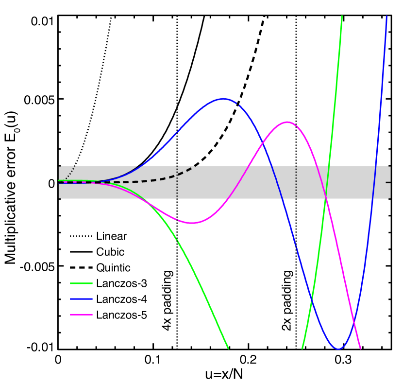
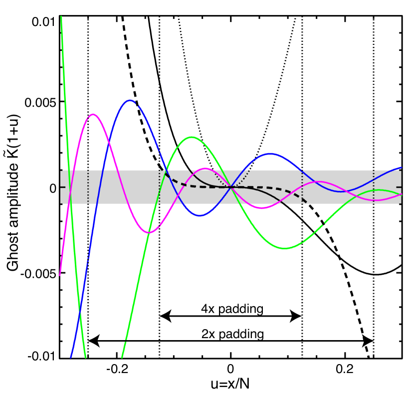
Figure 1: Error functions for several common interpolants. The left panel plots the multiplicative error $E_{0}(x/N)$ induced by approximation of the Fourier-domain sinc interpolation with the selected interpolant. The right panel plots the function $\tilde{K}(1+x/N)$ that gives the amplitude of the first, dominant, ghost image that is produced by using the chosen $u$-space interpolant. The vertical dotted lines show the maximum $x/N$ that will be present when the input data are zero-padded by a factor 2 or 4 before initial DFT. The horizontal grey band shows, for reference, errors of $\pm 1$ part per thousand. The polynomial filters (in black) obtain lower errors than the Lanczos filters (in colors) for given kernel size if $|u|<0.125$ is enforced by 4-fold zero padding.

Equivalent precision is available from the smaller cubic interpolant kernel if we precompute the DFT with 4-fold zero-padding to keep $|x/N|<\frac{1}{8}$. In this range we note that the cubic interpolant performs just as well as the Lanczos interpolants with larger (hence slower) kernels. This is attributable to the cubic interpolant being designed to be exact for polynomials of order $\leq 2$, which is equivalent to the requirement that $(d/d\nu)^{m}\tilde{K}(\nu)=0$ for integral $\nu$ and $m\leq 2$. Thus the cubic interpolant has $\tilde{K}(\nu)$ smaller than a Lanczos interpolant of equal size if we stay sufficiently close to integer values of $\nu$.

Inspired by the success of the standard cubic interpolant, we seek an interpolant that is exact for polynomial functions beyond quadratic order. This will require a 6-point interpolant, which must in turn be a piecewise-quintic polynomial function. This quintic filter, described in the Appendix, also has continuous second derivatives. The quintic interpolant indeed satisfies our expectation of performing extremely well if we confine the data to $\nu=x/N<\frac{1}{8}$ by a 4-fold zero padding of the data before the DFT. The multiplicative error $E_{0}(x/N)$ is $<5\times 10^{-4}$ in this case.

As an illustration of the second effect, the right panel of Figure 1 plots $\tilde{K}(1+u)$ for the interpolants, which determines the relative brightness of the first ghost image. We find essentially the same criteria on padding and choice of interpolant as we did from the threshold we imposed on $E_{0}$. This is assured, as $E_{0}(\nu)\approx\tilde{K}(1-u)+\tilde{K}(1+u)$, given that all filters beyond the linear one have $|\tilde{K}(2+u)|\leq 0.001$ for $|u|<0.25$. With 4-fold zero-padding, the polynomial filters are again the most efficient at reducing the amplitude of the ghost images. The 4-element cubic filter limits the ghost amplitude to 0.006 of the original $a_{j}$, and the 6-element quintic filter reduces the ghost amplitude to 0.0012.

Limiting both the amplitude of the ghost images and the multiplicative error on the central image of $\hat{F}(x)$ to be $<0.001$ is hence achieved by 4-fold zero padding of the input array, with a DFT followed by interpolation in $u$-space with the 6-point quintic interpolant. Similar performance is possible with the more compact 4-point cubic interpolant if the initial DFT has 6-fold zero padding.

The $O(N^{4})$ computational bottleneck at step 3 of our recipe can hence be replaced by $k^{2}N^{2}$ operations in convolution with an interpolant with $k\times k$ footprint, where $k=6(4)$ for the quintic (cubic) interpolant. The oversampling by factor $s=4(6)$ increases the time required for the input DFT (step 1) to $O(s^{2}N^{2}\log sN)$, leaving the DFT as the likely slowest step of the process. However the whole operation now scales, within constant/logarithmic factors, as the number of pixels in the input galaxy images. We note that if we are rendering many versions of a given input galaxy, it may be efficient to pre-compute and cache the oversampled input DFT. If storage space for this cache is not an issue, then the cubic interpolant with 6-fold DFT padding may be faster than quintic interpolant with 4-fold DFT.

Figure 2 shows the errors induced in reconstruction of a 2d bullseye image using three different $u$-space interpolation schemes.

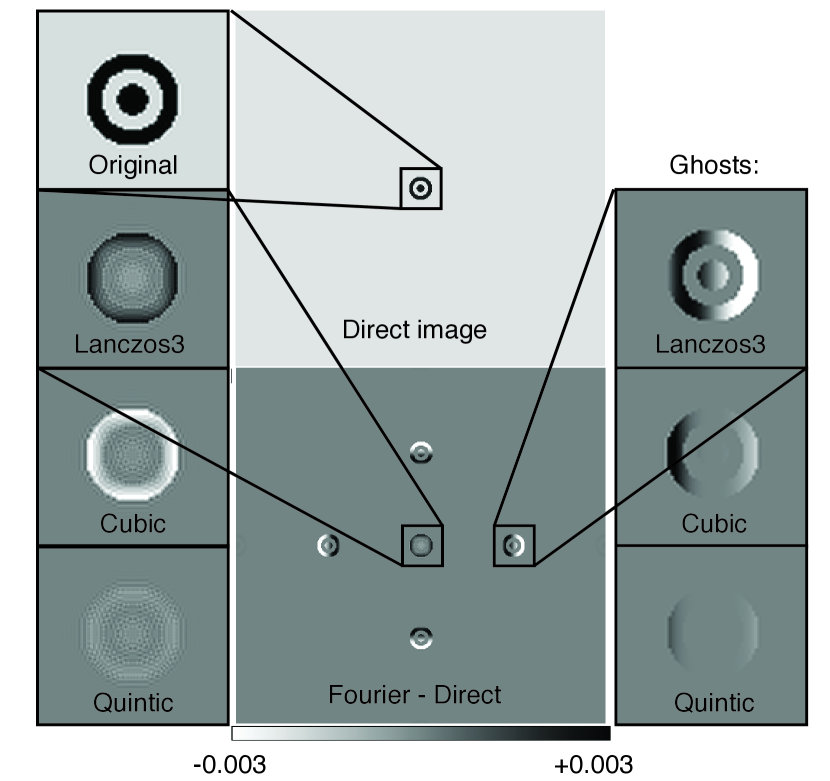
Figure 2: Errors induced by interpolation approximations in Fourier domain reconstruction of a 2d image. The original image is a $32\times 32$ pixel bullseye pattern with unit amplitude. The upper middle image, with close-up in upper left, is a $2\times$ oversampled rendition using a 3rd-order Lanczos function as the $x$-domain interpolant $K_{x}$. The original image is then zero-padded to $128\times 128$ pixels, DFT’ed to Fourier domain, interpolated to a new grid in Fourier domain with $K_{u}$ as a 3rd-order Lanczos filter, and transformed back to real space. The bottom middle panel is the difference between this reconstruction and the direct-interpolation image, showing the scaling error on the central image and the 4 dominant ghost images. The greyscale on the error images extends to $\pm 0.003\times$ the input image’s brightness. At left is the error in the central image; at right is a closeup of the right-hand ghost image. Changing the Fourier-domain interpolant from the $6\times 6$ Lanczos3 kernel, to a $4\times 4$ cubic interpolant, to a $6\times 6$ quintic interpolant leads to progressively smaller interpolation errors.

Table 1: Properties of Interpolants

Name	$N_{\rm points}$	$u_{\rm max}:$	Max reconstruction error for oversampling:
			$2\times$	$4\times$	$6\times$
			$x/N<1/4$	$x/N<1/8$	$x/N<1/12$
Nearest	1	317.5	(large)	(large)	(large)
Linear	2	9.6	0.18	0.049	0.022
Cubic	4	2.74	0.061	0.0061	0.0016
Quintic	6	3.62	0.037	0.0012	0.00015
Lanczos $n=3$	6	1.49	0.014	0.0035	0.0035
Lanczos $n=4$	8	1.35	0.005	0.0030	0.0019
Lanczos $n=5$	10	1.08	0.004	0.0022	0.0012
Sinc	$\infty$	0.5	0	0	0

Note. — Interpolants are defined in the Appendix. $N_{\rm points}$ is the number of grid points per dimension summed during the interpolation; $u_{\rm max}$ is the largest $|u|$ for which $|\tilde{K}(u)|>0.001$, giving some estimate of the power beyond the Nyquist frequency $u=0.5$ induced by the interpolant. The maximum of $|E_{0}(u)|$ and $|\tilde{K}(1\pm u)|$ attained for $u<x/N$ is listed for three values of $x/N$, corresponding to $2\times$, $4\times$, and $6\times$ zero-padding of the data, respectively.

4 Effect of wrapping

The above section considers the transform from $u$ space back to $x$ space to produce an output image $\hat{F}(x)$ to be continuous, but a discrete transform is necessary in practice. Consider this DFT to produce $M$ samples of the $x$-space image at spacing $\Delta x$. The DFT will sample the $u$ space at intervals $\Delta u=(M\Delta x)^{-1}$ to yield an output image that has been wrapped with period $P=M\Delta x$, such that the output point $\hat{F}_{j}=\sum_{k}\hat{F}(j\Delta x+kP)$. The input image $F(x)$ is confined to the extent $\pm N/2$ of the original input array $a_{j}$ plus the radius of the non-zero region for the interpolant $K_{x}$. Hence as long as the output DFT has extent $P>N$ that would contain the input image, the wrapped regions are nominally zero and the DFT yields an exact sampled representation of the output image.

However we must recall that, in the case where we have used an approximate interpolant $K_{u}$, ghost images are present in the output image at the locations $\pm N_{x}=\pm sN$, where $N_{x}$ is the size of the $x\rightarrow u$ input DFT, and $s$ is the zero-padding factor applied to the input data array with $N$ samples. If $P=N_{x}/n$ for some integer $n$, then the principal ghosts will be folded directly atop the primary image. This might seem damaging, but in fact means that the reconstructed $\hat{F}_{j}$ will be better, in fact perfect, because the summed ghost images will exactly cancel the multiplicative error $E_{0}(x/N_{x})$ that affects the primary image. Another way to see this is that if $P=N_{x}/n$, then the $u\rightarrow x$ DFT is using exactly the $u$ values produced by the $x\rightarrow u$ DFT, and no interpolation is being done at all.

Wrapping of the ghost images can be a major problem, though, in the following important application: suppose our goal is to take $F(x)$, dilate it to $G(x)=F[x/(1+\epsilon)]$, then convolve with some PSF function. This is, for example, exactly what one wants to do to simulate a sky that has been sheared by weak gravitational lensing—the image must be dilated by $\epsilon=\gamma$ in one direction and contracted with $\epsilon=-\gamma$ along a perpendicular axis. If we wish to execute this dilation in the Fourier domain, setting $\tilde{G}(u)=\tilde{F}[(1+\epsilon)u]$, then the ghosts will appear at locations $x\approx\pm(1-\epsilon)N_{x}$. If we do the $u\rightarrow x$ DFT with $P=N_{x}$, as might be common, then the ghosts are wrapped to positions $x=\pm\epsilon N_{x}=\pm\epsilon sN$, just slightly displaced. Figure 3 illustrates the results.

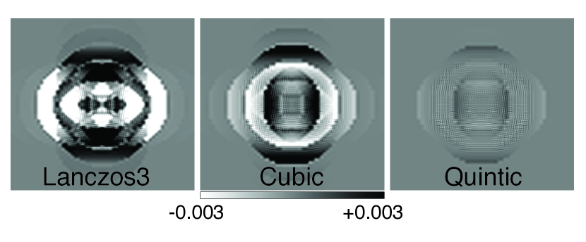
Figure 3: Errors induced by Fourier-domain interpolation in the case that we are simulating a shear of amplitude 0.1 on the bullseye image. The output DFT is done with period $P=128$ (equal to the zero-padded input $N_{x}$) such that the ghost images are wrapped atop the central bullseye, and these images show the resultant errors of the central image in closeup. The residuals are dominated by 4 copies of the ghost image, slightly shifted in the $\pm x$ and $\pm y$ directions because of the shear applied before the $u\rightarrow x$ DFT. The greyscale spans $\pm 0.003$ of the input bullseye brightness. The quadrupole patterns from the folded ghosts can confuse weak-lensing shear measurements in this case of unfortunate choice of DFT period, but the quintic filter is a great improvement on the Lanczos and cubic interpolants.

These displaced ghosts can generate spurious broadening of the reconstructed image $\hat{G}_{j}$. This is a problem when simulating sheared 2d sky images, because the interpolation errors induce a quadrupole moment atop that induced by the shearing of the image. We take our “bullseye” galaxy and calculate the ellipticity from unweighted quadrupole moments of the image:

$$M_{xx} \equiv \sum_{jk}\hat{G}_{jk}x_{j}x_{k}$$ (30)

$$M_{yy} \equiv \sum_{jk}\hat{G}_{jk}y_{j}y_{k}$$ (31)

$$e \equiv \frac{M_{xx}-M_{yy}}{M_{xx}+M_{yy}}.$$ (32)

The original bullseye pattern has a diameter of 32 pixels, and is $4\times$ zero-padded to 128 pixels before the $x\rightarrow u$ DFT. We construct a sheared image of this galaxy by interpolating in $u$ space and executing the $u\rightarrow x$ DFT on a $512\times 512$ grid with $\Delta x=0.25$. The quadrupole moment of this reconstruction is compared to that of an image constructed by direct interpolation of the $x$-space image with a 3rd-order Lanczos kernel. If the applied shear produces an ellipticity $e$ on the $x$-domain interpolation of the sheared image, we find that the reconstruction from cubic $u$-space interpolation produces an ellipticity that is systematically biased by about $0.04e$. The quintic filter is better, with biases of $\approx 0.004e$. If we increase the input zero-padding from $4\times$ to $6\times$, we find the quintic filter reduces spurious ellipticities to $<0.001e$, sufficient for highest-precision simulation of applied shear.

Note that the bullseye image is a worst case in the respect that it has full amplitude out to the edge of the initial domain. In practice we can expect postage-stamp images of galaxies to have near-zero flux at their edges. Since the ghosts of the quintic interpolation rise very rapidly at the edges, a typical galaxy or PSF cutout that has very little flux at the borders will have lower spurious contribution from wrapping of the ghost images.

5 Summary

We seek a recipe for performing high-precision Fourier-domain image simulation and analysis of galaxies and PSFs given as pixelized data, with values between the pixel samples specified by some interpolant $K_{x}$.

Our first question was: what is the exact expression for the Fourier transform $\tilde{F}(u)$ of such an interpolated, sampled image? Equation (11) gives the answer: first calculate the $\tilde{a}_{k}$ from a DFT of the input samples; then interpolate between the $u_{k}=k/N$ using a wrapped sinc function; then multiply by the transform $\tilde{K}_{x}(u)$ of the $x$-domain interpolant. The maximum frequency $u_{\rm max}$ with non-zero $\tilde{F}(u)$ hence depends on the choice of interpolant: $K_{x}={\rm sinc}(x)$ provides strictly band-limited $u_{\rm max}=0.5$ but produces an $F(x)$ that extends to very large distance beyond the original samples. The Lanczos interpolants are a good choice to define $F(x)$ that is not much larger than the original samples, while not extending $\tilde{F}(u)$ far beyond the original Nyquist frequency.

The sinc interpolation of the $\tilde{a}_{k}$ is often too slow for practical implementation at $O(N^{4})$, so how could we efficiently obtain the values $\tilde{F}(u)$ at arbitrary $u$ that are needed to implement simulation of sheared and convolved renditions of $F(x)$? Using a $u$-space interpolant $K_{u}$ that with a more compact kernel produces two errors in the simulated images: the first is a multiplicative error $E_{0}(x/N)$, where $N$ is the size of the $x\rightarrow u$ DFT and $E_{0}$ is a function characteristic of the interpolant $K_{u}$. The second error is the appearance of a pair of ghost images located $\pm N$ units from the original image, each ghost multiplied by the function $\tilde{K}_{u}(1\pm x/N)$, which is nearly the same size as $E_{0}(x/N)$.

Figures 1 and Table 1 show the size of these errors for common interpolants. We find that part-per-thousand accuracy on the resampled image and its ellipticity will be realized by the following recipe:

1. Zero-pad the input data by a factor 4 before performing the $x\rightarrow u$ DFT.

2. Use the $6\times 6$ pixel piecewise-quintic-polynomial interpolant in $u$ space.

We therefore recommend use of the quintic filter for $u$-space interpolation after zero-padding and DFT. The cubic filter can be used to gain a factor 2–3 in speed at expense of $\approx 5\times$ larger simulation errors, and these larger errors can be eliminated by 6-fold zero-padding of the input image.

There is one important caveat to this recipe: if the simulated $u$-domain image is transformed back to $x$ domain using a DFT with period $P$ that nearly evenly divides $N$, then the ghosts will be folded atop the primary image. A simulated shear or magnification will cause the ghosts to move relative to the primary image, which produces spurious broadening of the image, which can change the quadrupole moments of the image in a way that biases shear measurements. In a simple pessimistic trial case, we find that the standard $4\times$padding$+$quintic recipe induces 0.4% errors in a simple measure of applied shear, somewhat too big for testing state-of-the-art shear measurement techniques. We find it possible to reduce the spurious shear to $<0.001$ of the applied shear by combining the quintic $K_{u}$ with $6\times$ zero-padding of the initial DFT, which should be sufficiently accurate for foreseeable cosmic-shear simulations. In fact this would be overkill for most galaxy images that one is likely to be simulating, since they are already nearly zero at their edges and hence not in need of $6\times$ padding.

The methods described herein have been implemented as the core of the Fourier-domain image rendering code for the GalSim public-domain sky simulation code (Rowe et al., 2014).

Appendix A Function and interpolant definitions

We adopt the following conventions for functions and Fourier transforms:

$$\quad{\mbox{$\Pi$}}(x) \equiv \left\{\begin{array}[]{cc}1&|x|<0.5\\ 0.5&|x|=0.5\\ 0&|x|>0.5\end{array}\right.$$ (A4)

$${\mbox{\twlcyr Sh}}(x) \equiv \sum_{j=-\infty}^{\infty}\delta(x-j)$$ (A5)

$${\mbox{\rm sinc}}(x) \equiv \frac{\sin\pi x}{\pi x}$$ (A6)

$${\rm Si(x)} \equiv \int_{0}^{x}dt\frac{\sin t}{t}$$ (A7)

$$\tilde{f}(u) = \int_{-\infty}^{\infty}dx\,f(x)e^{-2\pi iux}$$ (A8)

$$f(x) = \int_{-\infty}^{\infty}du\,\tilde{f}(u)e^{2\pi iux}$$ (A9)

The interpolants considered in this paper are defined as follows:

• Nearest-neighbor: The real-space kernel is maximally compact, $K(x)=\Pi(x)$, but the Fourier domain $\tilde{K}(u)={\mbox{\rm sinc}}(u)$ extends to infinity as $\sim(1/u)$.

• Linear: Common interpolant with 2-point footprint in real space, and improved but still very broad Fourier behavior $\sim(1/u)^{2}$:

  $$K(x) = \left\{\begin{array}[]{cc}1-|x|&|x|\leq 1\\ 0&|x|\geq 1\end{array}\right.$$ (A12)

  $$\tilde{K}(u) = {\mbox{\rm sinc}}^{2}(u).$$ (A13)

• Cubic: Piecewise-cubic polynomial interpolant with continuous first derivatives designed to interpolate quadratic polynomials perfectly. This implies $\tilde{K}^{\prime}(j)=\tilde{K}^{\prime\prime}(j)=0$ for integers $j\neq 0$. The Fourier domain expression is analytic but too complex to merit detailing.

  $$K(x)=\left\{\begin{array}[]{cc}\frac{3}{2}|x^{3}|-\frac{5}{2}x^{2}+1&|x|\leq 1\\ -\frac{1}{2}|x^{3}|+\frac{5}{2}x^{2}-4|x|+2&1\leq|x|\geq 2\\ 0&|x|\geq 2\end{array}\right.\\$$ (A14)

• Quintic: A six-point interpolant that provides exact interpolation of fourth-order polynomial functions, and hence has $\tilde{K}(j\pm\nu)\sim\nu^{5}$ for $j\neq 0$, can be produced from a piecewise-quintic polynomial kernel. This kernel also has continuous second derivatives:

  $$K(x)=\left\{\begin{array}[]{cc}1+\frac{x^{3}}{12}\left(-95+138x-55x^{2}\right)&|x|\leq 1\\ \frac{(x-1)(x-2)}{24}\left(-138+348x-249x^{2}+55x^{3}\right)&1\leq|x|\leq 2\\ \frac{(x-2)(x-3)^{2}}{24}\left(-54+50x-11x^{2}\right)&2\leq|x|\leq 3\\ 0&|x|\geq 3\end{array}\right.\\$$ (A15)

• Lanczos: at order $m$ truncates the sinc filter after its $m$th null:

  $$K(x) \equiv {\mbox{\rm sinc}}(x){\mbox{\rm sinc}}(x/m)\Pi(x/2m)$$ (A16)

  $$\tilde{K}(u) \equiv 2m^{2}\Pi(u)\ast\Pi(u/m)\ast{\mbox{\rm sinc}}(2mu)$$

  $$= \pi(2mu-m-1){\rm Si}(2mu-m-1)-\pi(2mu-m+1){\rm Si}(2mu-m+1)$$

  $$-\pi(2mu+m-1){\rm Si}(2mu+m-1)+\pi(2mu+m+1){\rm Si}(2mu+m+1)$$

  Abramowitz & Stegun (1965) present approximations to the Si function which are very useful for calculating $\tilde{K}$ for the Lanczos interpolants or for estimating leading-order behavior of the interpolation error quantities described in this text. See their (5.2.6), (5.2.34), and (5.2.38).

  As noted in §3.1, the Lanczos filters do not conserve background flux, but in practice can be modified to do so. The plots and table assume that we are using background-conserving versions of the Lanczos filters.

• Sinc: conjugate of the nearest-neighbor filter, with $K(x)={\mbox{\rm sinc}}(x)$ and $\tilde{K}(u)=\Pi(u)$.