Real-time correlation reference update for astronomical adaptive optics

Abstract

The use of laser guide stars in astronomical adaptive optics results in elongated Shack-Hartmann wavefront sensor image patterns. Image correlation techniques can be used to determine local wavefront slope by correlating each sub-aperture image with its expected elongated shape, or reference image. Here, we present a technique which allows the correlation reference images to be updated while the adaptive optics loop is closed. We show that this can be done without affecting the resulting point spread functions. On-sky demonstration is reported. We compare different techniques for obtaining the reference images, and investigate performance over a wide range of adaptive optics system parameters. We find that image correlation techniques perform better than the standard centre-of-gravity algorithm and are highly suited for use with open-loop multiple object adaptive optics systems.

1 Introduction

All ground-based astronomical telescopes perform science by observing through the Earth’s atmosphere, which has a degrading effect on the images obtained. Adaptive optics (AO) (Babcock, 1953) is a technology employed on most major telescopes, which seeks to remove some of the effects of atmospheric turbulence, producing clearer, high resolution science images as a result. It is a crucial technology for the next generation Extremely Large Telescope (ELT) facilities which will spend the significant majority of their time producing AO corrected observations.

The field of view of high image quality obtained from a classical AO system (Babcock, 1953) (around the guide star that is used to sense the atmospheric turbulence), is limited by the atmospheric isoplanatic patch size, typically a few seconds of arc in diameter. This results in degrading image quality for science targets away from this guide star position. Wide field adaptive optics systems have recently been commissioned (for example, CANARY, Gendron et al. (2011)) which increase the corrected field of view by using multiple guide stars and performing a tomographic reconstruction of the atmospheric turbulence. Herein lies a problem: there are only a limited number of stars with sufficient brightness that form asterisms with the small angular separation required for wavefront sensing for wide field AO. Therefore, sky coverage of such systems is limited.

Sky coverage is improved by the use of laser guide stars (LGSs) (Foy & Labeyrie, 1985), which allow artificial star asterisms to be placed anywhere on the sky though sky coverage is still limited by the requirement that at least one natural guide star (NGS) is necessary to overcome tip-tilt uncertainty.

Most astronomical AO systems use Shack-Hartmann wavefront sensors (Shack, 1971). With NGSs, an array of Airy disc spots is produced because the source is unresolved. However with LGSs these spots are elongated, as demonstrated in Fig. 1, due to the geometrical effect of viewing an extended source off-axis.

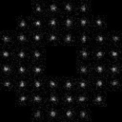
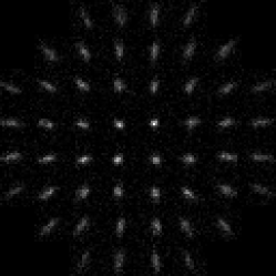
Figure 1: (a) A figure showing a typical Shack-Hartmann spot pattern for a natural guide star. (b) For a laser guide star. (c) Showing a typical non-uniform sodium layer density profile (Butler et al., 2003).

Shack-Hartmann wavefront sensors estimate the local wavefront gradient or slope in each sub-aperture by measuring the offset of the individual spots from a reference position defined by their position when a flat wavefront is incident on the wavefront sensor. A centre of gravity (CoG) measurement can provide an essentially unbiased estimate (depending on sampling, signal and background levels, and field of view) for circularly symmetric NGS spots. However for elongated LGS spots, this is not the case if field of view or flux are limited (i.e. any practical situation). This is because signal and noise are spread unevenly along the elongated and un-elongated directions, and hence noise propagation is different along these directions which can affect wavefront reconstruction. Spot truncation in the direction of elongation can also occur, resulting in biased slope measurements, particularly if the spot is under sampled. This is compounded for Sodium LGSs (Foy & Labeyrie, 1985) by the non-uniform profile of the Sodium layer density in the upper atmosphere which causes Sodium LGS spots to be non-smooth (Fig. 1), introducing complications for spot offset measurements. Likewise, for Rayleigh LGSs (Thompson & Castle, 1992), it can be necessary to increase the optical range-gate depth to increase photon flux in poor seeing conditions, leading to greater spot elongation, which can again lead to complications for wavefront sensor (WFS) slope measurement.

A solution to the spot elongation problem is to compute the correlation of the LGS spots with a reference image (Thomas et al., 2006), and then find the CoG of this correlation image, thus giving the spot offset. This naturally leads to the question of how to obtain a suitable reference image, which will be different for each sub-aperture. This form of slope estimation is commonly used for solar AO (Richards, 2012), where the Shack-Hartmann images have a very different structure, and an identical reference for each sub-aperture can be used. Correlation is usually performed using a two dimensional Fast Fourier transform to reduce computational complexity. For night-time astronomical AO, the reference images differ in each sub-aperture due to the geometrical nature of the spot elongation.

1.1 Solar adaptive optics wavefront sensing

Solar AO systems use this correlation technique for wavefront sensing. The reference image used is identical for each sub-aperture, and is typically chosen from a single sub-aperture in a single frame of Shack-Hartmann images, updated approximately every 30 seconds. This reference image updating is necessary because the Sun’s surface is constantly changing, and so the correlation between a given Shack-Hartmann image and the reference decreases with time, reducing the AO system correction quality. Updating the reference image in this way will cause the science image to change position, since this reference image changes for all sub-apertures, and thus introduces an identical constant wavefront slope offset for each sub-aperture. However this is not a problem for solar AO because the integration times for the science images are typically only a few seconds (otherwise image saturation will occur). Therefore, update of the correlation reference image can be synchronised with a new science image exposure.

1.2 Key differences for astronomical correlation wavefront sensing

The situation for night-time astronomical AO correlation wavefront sensing is more complicated. A single reference image cannot be used because the shape of each Shack-Hartmann spot is different (defined in part by the distance and angle of the sub-apertures from the laser launch axis). Therefore, a unique correlation image for each sub-aperture must be supplied.

Astronomical AO systems generally work in the photon-starved regime, where fluxes and signal-to-noise ratios are low. This is generally also the case when using LGSs primarily because of the increasing cost of more powerful lasers, the desire to operate with high frame rates and at high WFS order. A single frame LGS image is therefore generally noisy, and so the computation of correlation reference images cannot be obtained from a single frame of Shack-Hartmann data since flux is low, and such images would contain significant noise. Rather, it is necessary to integrate wavefront sensor images for long enough to provide a reference image with a high signal to noise ratio, but over a time period short enough to ensure that the Sodium layer density profile has not changed significantly to avoid blurring of the reference images. Wavefront sensor images spanning of order one second of time would seem to be a reasonable compromise (as we will show), though this will depend upon the AO system in question, the Sodium layer variability (which is not constant) and the lasers.

Finally, science integration times for astronomical instruments are far longer than those for solar observations. Therefore it is not possible to only update the correlation reference images in between science exposures, since the time interval is too long and the correlation reference images would quickly become out of date leading to poor AO performance.

This paper presents a solution to these problems, with on-sky testing reported using the CANARY demonstrator instrument on the William Herschel Telescope. This is of crucial importance for future ELT multi-object AO (MOAO) systems where wavefront sensing is performed in open-loop. When operating in open-loop, wavefront sensors do not see the effects of changes made to deformable mirror (DM) shape, and therefore spot motions can be large. Other wavefront sensing algorithms, such as a weighted CoG or matched filter algorithms (Thomas et al., 2006) are non-linear and so work only poorly for open-loop wavefront sensing. The use of a correlation algorithm gives significant performance advantages over a basic CoG algorithm (Thomas et al., 2006), while still maintaining the linearity essential for open-loop systems.

In §2 we present a technique for updating the correlation reference images in an astronomical AO system whilst maintaining engagement of the AO loop, without affecting science image quality. In §3 we give details of our implementation of this technique and results obtained both from simulation and on-sky. Finally in §4 we draw our conclusions.

2 Real-time update of correlation reference images

There are several techniques that can be used to obtain suitable correlation reference images from noisy WFS images, which we now discuss.

2.1 Generation of correlation reference images

2.1.1 Integration of wavefront sensor images

The first technique to obtain correlation reference images is to simply sum a suitable number of LGS wavefront sensor image frames, for each sub-aperture. The number of image frames should be chosen to achieve a good signal-to-noise ratio, while remaining low enough that the Sodium profile remains approximately constant during this time, and we suggest that of order 0.1-1 s is appropriate. However, the drawback of this simple approach is due to the atmosphere itself, which will cause blurring of the integrated image due to spot movement between frames. Therefore, the correlation reference images will not be optimal.

2.1.2 Shifting and adding

The second technique that can be used to obtain correlation reference images is to shift and add WFS images from a number of individual frames (again, probably spanning of order one second) on a per-sub-aperture basis (i.e. with potentially a different shift for each sub-aperture). To use this technique, the position of each spot in each frame is determined. These spots are then shifted to the position corresponding to zero (either using an integer pixel shift or using sub-pixel interpolation), and summed with the corresponding spots from other image frames.

The determination of the spot position can be made (on a per-sub-aperture basis) either using a simple CoG estimation, or by correlating with the current reference images, or by correlating with a model of the spots.

2.1.3 Modelling

A further technique which can be used to obtain the reference images is using modelling. A small number of LGS wavefront sensor images can be obtained, and these used to derive parameters for a model of the Sodium layer density profile, for example number and separation of sodium density peaks. Alternatively, an external profile monitor could be used. This model can then be used to generate suitable correlation reference images. We do not consider this modelling approach further here, rather concentrating on data driven approaches.

2.2 Updating the reference images

A flat incoming wavefront does not usually correspond to wavefront slope measurements of zero. Rather, it is necessary to perform a calibration to measure a set of reference slope measurements that correspond to a flat wavefront on the science image, leading to best AO corrected image improvement. Changing the correlation reference images will lead to different slope measurements for a given wavefront, and therefore it is necessary to obtain a different set of reference slopes for each set of correlation reference images. If the correlation reference images are uploaded to a real-time control system without further considerations (i.e. without also modifying the reference slopes), the AO corrected science image point spread function (PSF) will change each time, leading to poor performance. This is because the zero point (the estimated spot location for a flat input wavefront) changes depending on the correlation reference. The solution which we propose is therefore to update the reference slope measurements at the same time as the reference correlation images. We here outline the method by which these correlation reference slopes can be obtained, which is also demonstrated in Fig. 2. This is key to operating a correlation based wavefront sensor with a night-time astronomical AO system.

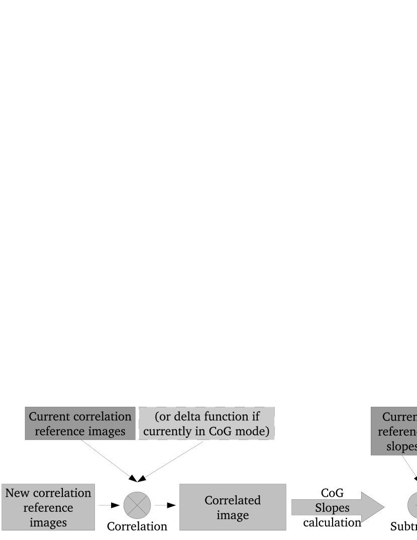
Figure 2: A diagram showing the technique used to obtain reference slope measurements, and thus enable simultaneous updating of correlation reference images and reference slopes during closed-loop operation.

2.3 Reference slope calculation

We define the “Initial Reference Slopes” as those that give the best science PSF when a CoG centroiding algorithm is used. Here, we note that correlation of an image with a two dimensional delta function (i.e. an array of zeros, with a value of one in the centre) yields the image itself, and so the CoG centroiding algorithm yields the same result as correlation with this identity followed by a CoG calculation.

We can compute the new reference slopes that will be required when the first set of correlation reference images are to be used, as follows (assuming that the system is previously using CoG or correlation with a delta function). We calculate the correlation of the new reference images with a delta function. The centroid measurements of the resulting correlation images are then obtained, and these values subtracted from the “Initial Reference Slopes”, to give the new reference slopes to be used alongside the new correlation reference images. Strictly speaking the correlation is unnecessary here, however it has been included for completeness, when comparing with the next section.

When a further update of correlation reference images is required, this process can be repeated: The correlation of the new images with a delta function is calculated, and the centroid measurements of these correlations obtained. These centroid measurements are then subtracted from the “Initial Reference Slopes” (not the reference slopes currently in use), giving the new reference slopes to be used with the new correlation reference images.

2.3.1 Initial Reference Slope ignorance

It is entirely possible that the “Initial Reference Slopes” are not known. This could be because the science PSF has been optimised with correlation reference images already in use, because an automatic ongoing optimisation of reference slopes is in place, or for other reasons. In this case, it is not possible to follow the preceding procedure for reference slope calculation, and some modifications are required as follows.

Rather than computing the correlation of the new reference images with a delta function, the correlation of new and current reference images is computed. The centroid measurements of these correlations are obtained, and these values subtracted from the reference slopes that are currently in use (not the “Initial Reference Slopes”), to give the new reference slopes, which can then be used alongside the new correlation reference images.

It should be noted that this scheme only relies on knowing the current correlation reference images, and the current reference slope measurements, both of which are easily obtainable from a real-time control system. No other state information is required (e.g. the “Initial Reference Slopes”), and so this technique is more robust against operator error, for example the “Initial Reference Slopes” being out of date.

When using this scheme, it may be possible for errors in reference slopes to build up over time, something we investigate further in this paper (§3.3). This can arise because each time a new set of reference slopes are computed, there is a reliance on the new and current correlation reference images both of which will have some noise, and so each successive set of reference slopes will have increased noise.

2.4 Background complications

Accurate calculation of wavefront slopes from correlation images is dependent on correct treatment of image background levels. In solar AO, where the sub-aperture images are extended it is necessary to use a windowing function, such as a Hamming window when performing the correlation to reduce edge effects. In astronomical AO, such a windowing function is not necessary if background levels are correctly removed and the Shack-Hartmann sensor (SHS) spots do not fill the sub-apertures . However, if the background level is not correctly removed, or significant detector noise is present, difficulties remain. In this case, the correlation image can have a significant background level, which will bias the slope measurement unless treated correctly.

As a solution for this, we suggest the use of a brightest pixel selection algorithm (Basden et al. (2012)(a)), for which the $n_{\mathrm{i}}$ brightest pixels in the $i^{\mathrm{th}}$ sub-aperture are selected for further processing, and the background level is set at the value of the $n_{\mathrm{i}}+1^{\mathrm{th}}$ brightest pixel in this sub-aperture. This has been shown to significantly reduce the effect of variable backgrounds and the impact of readout noise. The use of this algorithm is assumed throughout this paper unless otherwise stated, and a value of 40 is considered typical for $n_{\mathrm{i}}$ here, i.e. only the 40 brightest pixels in each sub-aperture are selected for processing, the rest being set to zero. It should be noted that this is only sensible for sub-apertures that contain more pixels than this. By using this algorithm, we are able to remove much of the background level from our correlation images, allowing an improved estimation of wavefront slope to be made.

2.5 Zero-padding and computational requirements

When Shack-Hartmann spots are extended with dimensions that are a significant fraction of the sub-aperture size, it is necessary to zero-pad the sub-aperture images before calculation of the image correlation when using the Fast Fourier transform correlation method. If this is not performed, the correlated image may wrap around at the boundaries, producing a significant bias for slope estimation, as shown in Fig. 3.

The computational complexity of a two dimensional Fast Fourier transform scales as $\mathcal{O}(n^{2}\ln n)$ for images with side dimension $n$. Additionally, common Fast Fourier transform algorithms perform better for certain image sizes, notably those with a side length equal to a power of two. Therefore, it is advantageous for a real-time system to be able to have varying degrees of zero-padding, depending on reference image size to reduce computational requirements. With a LGS system, variation in reference image spot size with distance from the laser launch axis allows computational savings to be made by varying the sub-aperture sizes, or amount of zero-padding, depending on expected elongation. Once the correlation has been performed, the image size, and therefore the computational effort in the CoG computation, can be reduced by clipping the correlation images.

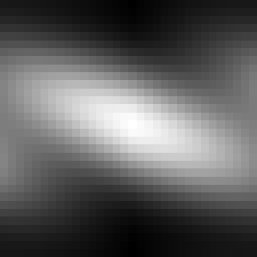
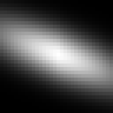
Figure 3: (a) A correlation of a single sub-aperture with the corresponding correlation reference without zero padding. The image wrapping can be clearly seen, affecting slope estimation. (b) As (a) but with the inclusion of zero padding. No image wrapping occurs.

2.6 Real-time control implementation

Real-time control for AO is computationally demanding, particularly for ELT scale systems, since WFS images must be processed and the DM demands computed within short timescales. The use of correlation wavefront sensing, requiring the computation of many small image correlations in a short period of time further adds to the computational demands placed on the real-time control system. In this section, we describe the real-time implementation of correlation wavefront sensing that is implemented in the real-time control system used with our on-sky demonstration instrument.

2.6.1 DARC

The Durham adaptive optics real-time controller (DARC) (Basden et al., 2010) is a high performance, central processing unit (CPU) based real-time control system for AO, which has been used successfully on-sky with CANARY. DARC has a modular design which affords it great flexibility for developing and testing new algorithms. An advanced correlation wavefront sensing module has been developed, and used both on-sky and for this investigation. The suitability of DARC for use with ELT-scale AO systems has been demonstrated (Basden & Myers (2012)(b)), and includes the ability to make use of additional computational hardware including field programmable gate arrays (FPGAs), graphical processing units (GPUs) and the Intel Xeon Phi, a many-core hardware accelerator.

The DARC system has the ability to use rectangular sub-apertures that are positioned and sized arbitrarily, i.e. a regular grid-like pattern is not required. This allows sub-apertures to be sized according to expected spot elongation which varies across the telescope pupil, thus reducing computational requirements. The correlation of each sub-aperture with an associated reference image is performed using a Fast Fourier transform algorithm, with intermediate steps stored in half-complex format (being Hermitian), thus reducing memory bandwidth requirements. Arbitrary zero-padding can be defined, in either dimension, on a per-sub-aperture basis, allowing performance savings to be made when spots are small relative to sub-aperture size, and ensuring that aliasing of the Fast Fourier transforms does not occur.

A (weighted) CoG algorithm is used to measure the centroid of the correlation image, which can be clipped to reduce computational requirements, particularly when zero-padding has been implemented. Alternatively, a two dimensional parabolic or Gaussian fit to the correlated image can also be used to determine wavefront slope, though this is not discussed further here.

2.6.2 Reference image and slope update

DARC has the ability to allow synchronous update of parameters on a per-frame basis. Our graphical on-sky correlation tool allows reference images to be obtained (averaging calibrated WFS images), and from these, updates to the current reference slope measurements are computed, as detailed in sections following §2.2. The new reference images are then uploaded at the same time as the new reference slopes, allowing the AO loop to remain closed (or engaged, for open-loop systems) while this operation is performed.

2.7 Sodium layer variability

It is important to realise that this technique does not solve the Sodium layer variability problem (Davis et al., 2006), which arises because of uncertainty in the time-varying profile of Sodium layer density. However, what it does allow is for a continual optimisation of WFS performance by matching the reference images as closely as possible to the true Sodium layer density profile.

In the case that an optical range gate can be applied to the Sodium layer return signal (i.e. a pulsed laser and a fast WFS shutter to only image pulses of light returning from a certain height in the atmosphere), then the uncertainty due to Sodium layer variability can be removed. The technique presented here then has a greater effect improving wavefront slope measurements even in the presence of changing Sodium layer density profiles.

2.8 On-sky validation of reference update

The technique proposed here for simultaneous update of correlation reference images and slopes has been tested on-sky during the night starting on 25th May 2013 using the CANARY multiple LGS AO system. During these tests, with CANARY operating in a MOAO mode, the reference images and slopes were updated while the AO loop remained active. We recorded AO corrected PSFs obtained while using a CoG slope estimation algorithm, and then while using the correlation algorithm, with four successive correlation reference image updates. Finally a further AO corrected PSF was obtained while using a CoG algorithm for slope estimation.

Some variation in Strehl ratio is expected due to the variability of atmospheric turbulence strength. However, as shown in Fig. 4, we do not see a continual worsening of performance for consecutive reference updates. We therefore conclude that our technique of updating the correlation reference images on-sky works well, thus mitigating some of the risk attached to ELT scale LGS AO systems. This figure spans a period of about five minutes close to dawn, and the AO performance obtained using correlation is shown to be better than that using the CoG algorithm (taken both before and after the four consecutive correlation updates). The standard CANARY data processing tool was used to obtain these measurements.

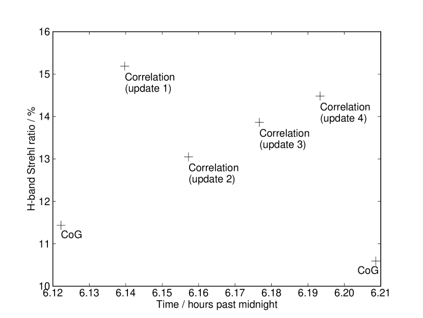
Figure 4: A figure showing AO corrected Strehl ratio as a function of time when using both a CoG algorithm, and correlation algorithm (with successive updates of the correlation reference images while the AO loop was active). These data were recorded using the CANARY instrument on the night starting 25th May 2013 (so the data themselves are from the 26th May).

3 Reference image technique comparisons

To investigate the correlation reference update techniques detailed in the preceding sections, we have used the Durham AO simulation platform (DASP) (Basden et al., 2007). We have interfaced this simulation tool with DARC, providing a hardware-in-the-loop simulation capability (Basden, 2014). Our approach is as follows:

1. A sequence of noiseless, atmospherically propagated LGS elongated SHS spot patterns is generated.

2. Photon shot noise, and detector readout noise is introduced to these images.

3. These images are passed into the real-time control system, DARC.

4. Correlation reference images are obtained using a number of these calibrated WFS images, either the mean image, by shifting and adding, or by interpolating as described previously.

5. A new, independent, set of noiseless and noisy LGS SHS spot patterns are generated. The correlation algorithm is used to estimate the WFS slope measurements using the noisy spot patterns, and these slope measurements are compared with the known (noiseless) slopes. A CoG algorithm is also used with the noisy spot patterns for performance comparisons.

Our performance metric is the root-mean-square (RMS) difference between estimated and true slope measurements. This technique is demonstrated in Fig. 5. Although the visual difference between the different techniques for reference image creation is small (Fig. 6), the following results show that the technique used is worthy of consideration.

Figure 5: A diagram showing our simulation approach. Laser guide stars are propagated through the atmosphere, and Shack-Hartmann images formed, with photon noise and readout noise. These images are passed to an instance of DARC, which processes them, providing wavefront slope measurements. These slope measurements are then compared with the true slope measurements.

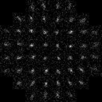
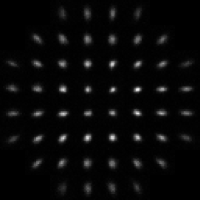
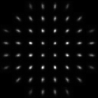
Figure 6: (a) A figure showing a simulated Laser Guide Star Shack Hartmann image, with a mean signal of 200 photons per fully illuminated sub-aperture, and a read-out noise of two electrons. (b) A reference image computed from the sum of 100 SHS images. (c) A reference image computed from 100 SHS images shifted and added. (d) A reference image computed from 100 SHS images interpolated and shifted, then summed.

3.1 Simulation parameters and method

DASP is a Monte-Carlo time-domain simulation code, which models the atmosphere using a series of translating phase screens, and uses physical optics for modelling the telescope and optical components. Here, we simulate wavefront sensor images based on a $8\times 8$ sub-aperture SHS on a 3.93 m telescope. We use a 90 km laser beacon with a Sodium layer depth of 30 km and a Gaussian profile. Although such a depth is unrealistic, it allows us to simulate the extreme elongation that would be seen at the edge of an ELT instrument, as well as less elongated spots from close to the laser launch position, and therefore our results are relevant for these future telescopes. A simulated spot image is shown in Fig. 6(a), covering a range of spot elongations due to different off-axis viewing angle. Unless otherwise stated, we do not vary the Sodium profile in our simulations. This does not significantly affect our results, because we concentrate on short periods of time (typically less than a second), over which the profile would not change significantly, and also show that the correlation reference can be updated whilst the AO loop is closed without affecting performance, i.e. results will not be affected when the profile does change. Although DASP is suitable for ELT-scale simulation (Basden et al., 2010; Basden et al., 2013), it would take a prohibitive amount of time to perform the investigations that we carry out here at these scales. We therefore approximate, using sub-apertures of the same size as those expected on the European ELT (E-ELT) (about 0.5 m), and spot elongations that cover the range of those expected on the E-ELT.

Unless otherwise stated, we assume a mean WFS signal of 200 photons per fully illuminated sub-aperture per frame, and a readout noise of two electrons, and assume $16\times 16$ pixels per sub-aperture. We model the atmosphere with a Von Karman model using an outer scale of $L_{0}=50$ m, and a Fried’s parameter of $r_{0}=10.6$ cm, and have a 4 ms WFS integration time. We assume that 70% of the turbulence is at the ground layer, with 30% at 11 km, though since we are not performing any wavefront reconstruction, our results are not dependent on atmospheric profile (though spot broadening will occur for worse seeing). We use a wavefront sensor pixel scale of 0.25 arcsec per pixel, with a sub-aperture field of view of 4 arcsec.

Results are shown for the most elongated LGS spots at $45^{\circ}$ unless otherwise stated, and we find that our results do not greatly depend on degree of elongation. For computation of the correlation reference images, we use 100 SHS image frames, as found to near-optimal in §3.2.5 (unless stated otherwise), and the slope estimation inaccuracies are computed using an ensemble of 10000 frames.

3.2 Investigation of results

3.2.1 Investigation of correlated image clipping

Oversampling of the reference images to avoid aliasing (wrapping) leads to larger correlation images. Clipping rows and columns from the edges of these correlated images not only cuts out any noise present in the edges, but also reduces computational requirements for the resulting slope estimation. Fig. 7 shows slope estimation accuracy as a function of clipping (equal to the number of rows and columns removed from each edge). In this instance, a clipping of eight returns the image to its pre-correlation size ($16\times 16$ pixels), and is seen to give best slope estimation. In this case, the signal level is 200 photons per fully illuminated sub-aperture per WFS integration, and readout noise is two electrons. At higher signal to noise ratio (SNR) levels, clipping does not lead to such a marked improvement, however we recommend that clipping should be used as performance is never seen to be worse. 100 WFS images were used to create the correlation reference images in this case.

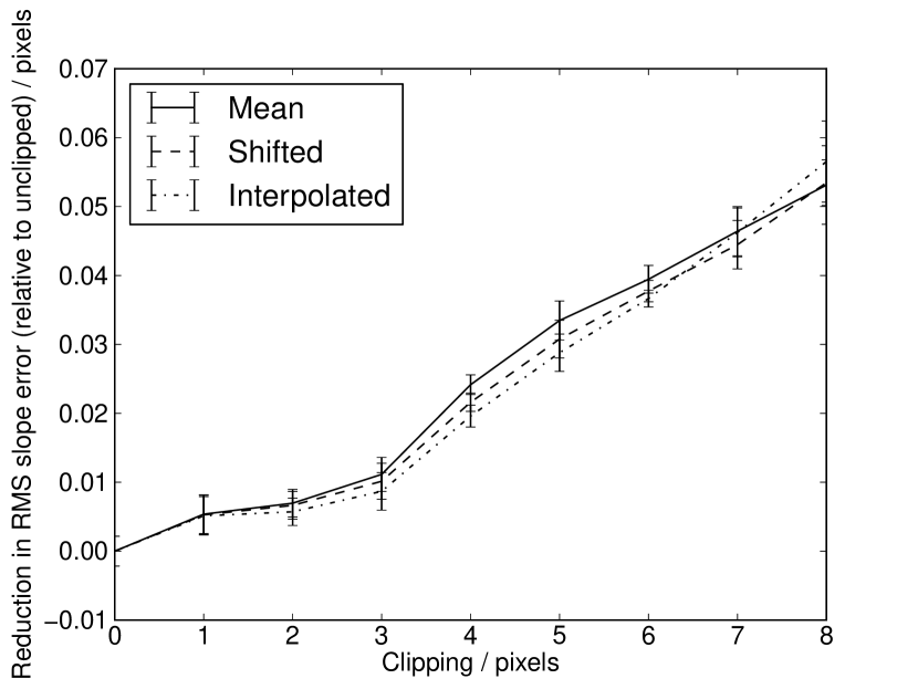
Figure 7: A figure showing improvement in slope estimation as the clipping of correlated images is increased. Here, the signal level is 200 photons per fully illuminated sub-aperture per integration, with a camera readout noise of 2 electrons. The reduction in slope error is displayed relative to the error from unclipped correlated images, so that higher values signify improved slope estimation.

3.2.2 Investigation of background removal

We have investigated background level subtraction using both a conventional constant background level, and also using the brightest pixel selection technique (with no prior background removal).

Fig. 8 shows performance (slope error) of correlation and CoG algorithms as a function of threshold level above the mean background. Here, the mean signal is 200 photons per pixel per unvignetted sub-aperture, and the readout noise is two electrons. The threshold level is subtracted from all pixels, and any negative values are then set to zero. Best performance is seen with a threshold level of two sigma (four electrons) above the mean, when using correlation with elongated spots (far from the laser launch axis), while a higher threshold level gives better performance for less elongated spots (sub-apertures closer to the laser launch axis). It is interesting to note that if the threshold level is set too low for highly elongated spots then the CoG algorithm performs better.

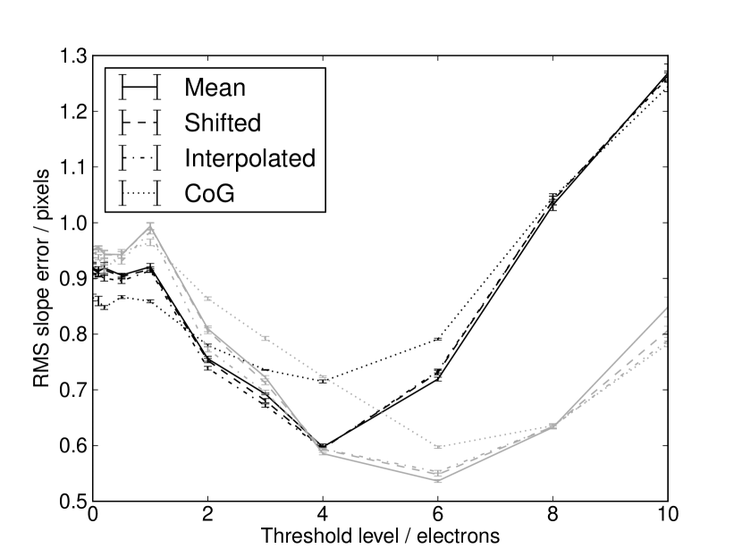
Figure 8: A figure showing slope estimation error as a function of background level above mean background. Here, the signal level is 200 photons per fully illuminated sub-aperture per integration, with a camera readout noise of 2 electrons. The black curves are for sub-apertures displaying large elongation, while grey curves are for sub-apertures close to the laser launch axis. Lower values represent better performance.

Fig. 9 shows slope estimation error as a function of number of brightest pixels selected for further processing for a WFS with a mean of 200 photons per pixel per unvignetted sub-aperture, and a detector readout noise of two electrons. It has been shown that the optimum number is dependent on spot size (Basden et al. (2012)(a)), and unless otherwise stated through out this paper, we use a default value of 40, which is close to minimum in this case, and provides near optimum performance over the range of signal levels, readout noise and spot sizes considered here. Fig. 9 shows that correct background subtraction leads to improved performance for correlation techniques over CoG. It should be noted that the background subtraction based on brightest pixel selection provides better performance than using a fixed background level, in part because it provides an automatic way to vary background level across the WFS camera.

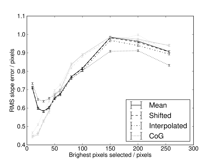
Figure 9: A figure showing slope estimation error as the number of brightest pixels per sub-aperture selected for further processing is changed. Here, the signal level is 200 photons per fully illuminated sub-aperture per integration, with a camera readout noise of 2 electrons. The black curves represent highly elongated spots at the edge of the pupil, at 45^∘, while the grey curves represent spots close to the launch axis, having less elongation. Lower values represent better performance.

3.2.3 Investigation of readout noise

Increasing readout noise reduces AO performance. However, as shown in Fig. 10, correlation WFS performance improves relative to CoG performance as noise increases (although, of course, slope estimation accuracy itself reduces). This highlights the benefits of correlation WFS algorithms at lower signal-to-noise ratios, and also shows that reference images produced using interpolation provide better performance at the lowest signal-to-noise ratios.

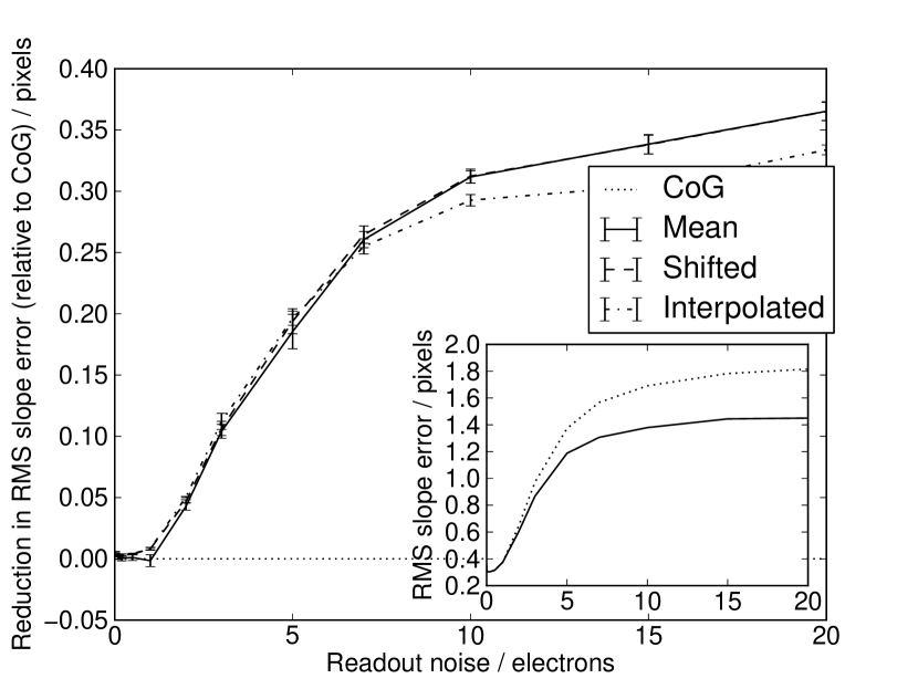
Figure 10: A figure showing the reduction in slope estimation error relative to CoG as a function of detector readout noise, with higher values signifying improved slope estimation. Inset is shown the actual slope error for the centre of gravity and correlation (using a mean reference) algorithm (here, higher values signify worse slope estimation). The signal level is 200 photons per unvignetted sub-aperture per frame.

3.2.4 Investigation of signal level

Fig. 11 shows the reduction in error of correlation WFS performance relative to CoG performance as a function of WFS signal level for different detector readout noise levels. It can be seen that at high light levels, the CoG and correlation performance is similar, while at lower light levels, correlation provides better performance than CoG. It should be noted that shifted and interpolated correlation reference images achieve better performance than correlation reference images obtained from the mean of the pixel data.

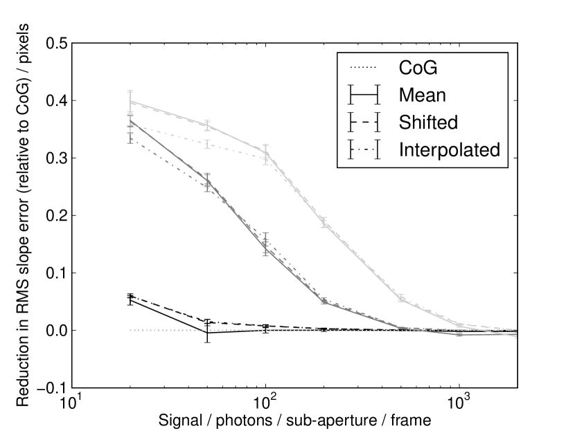
Figure 11: A figure showing the reduction in slope estimation error relative to CoG as a function of WFS signal. The readout noise is 0.1 electrons (black curves), 2 electrons (dark grey curves) and 5 electrons (light grey curves). CoG slope error reduction is always zero since we are displaying reduction relative to CoG, and positive values represent improved performance relative to CoG.

3.2.5 Investigation of number of reference frames

The number of SHS image frames used to compute the correlation reference images is of interest, regardless of the algorithm used to compute the reference from the raw images. Fig. 12 shows slope estimation error as a function of number of image frames used to compute the reference image. Here it can be seen that a sample of approximately 100 images gives best performance, though there is a fair degree of tolerance, particularly when using the interpolated reference calculation technique. The line for CoG is also shown for comparative purposes (since this does not require reference images). The RMS slope error is seen to increase after about 100 frames and this is due to increased spot blurring in the reference images, resulting in reference spots that resemble the actual median sub-aperture image less well.

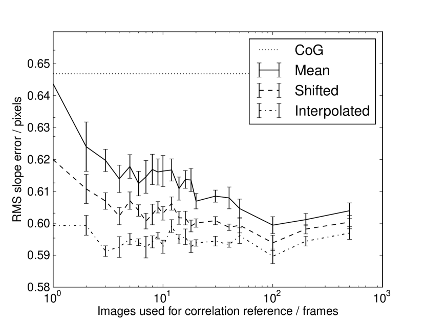
Figure 12: A figure showing slope estimation error as a function of number of images used to build the reference image. Here, the mean signal is 200 photons per sub-aperture with 2 electrons readout noise.

3.2.6 Investigation of threshold on correlated image

After the correlation of a SHS spot with the reference image has been computed, the resulting correlation image requires processing to yield the local wavefront slope estimate. Here we investigate the effect that applying a threshold to this correlated image has on the slope estimation accuracy. Fig. 13 shows slope estimation error as a function of the correlation threshold, where the threshold is given as a fraction of the maximum value in the correlation image. Here, we see that by selecting a threshold level that is a small fraction (0.1–0.2) of the maximum value in each sub-aperture we can improve the slope estimation accuracy.

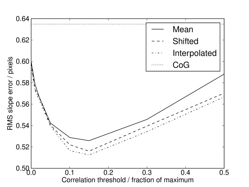
Figure 13: A figure showing slope estimation error as a function of correlation image threshold level.

It should be noted that this is a separate threshold level than that applied during image calibration. Applying a threshold to the correlated image helps to remove the effect of unwanted frequency components, increasing slope estimation accuracy. This also helps to negate the effect of an incorrect image calibration (i.e. an incorrect threshold applied to the raw image.

3.3 Reference slope noise propagation

As discussed in §2.3.1, it is possible (and sometimes necessary) to update correlation reference images and reference slopes using only a knowledge of the current system state. One major source of bias in reference slope estimation comes from clipping of the correlation reference images. It is essential that reference slope offsets are computed using the unclipped correlation of the current and new reference images. If this is not the case, i.e. the slope offsets are computed using a clipped correlation image, errors in these slope estimates quickly build up, as shown in Fig. 14. When computed correctly, we do not see errors build up, even over long timescales.

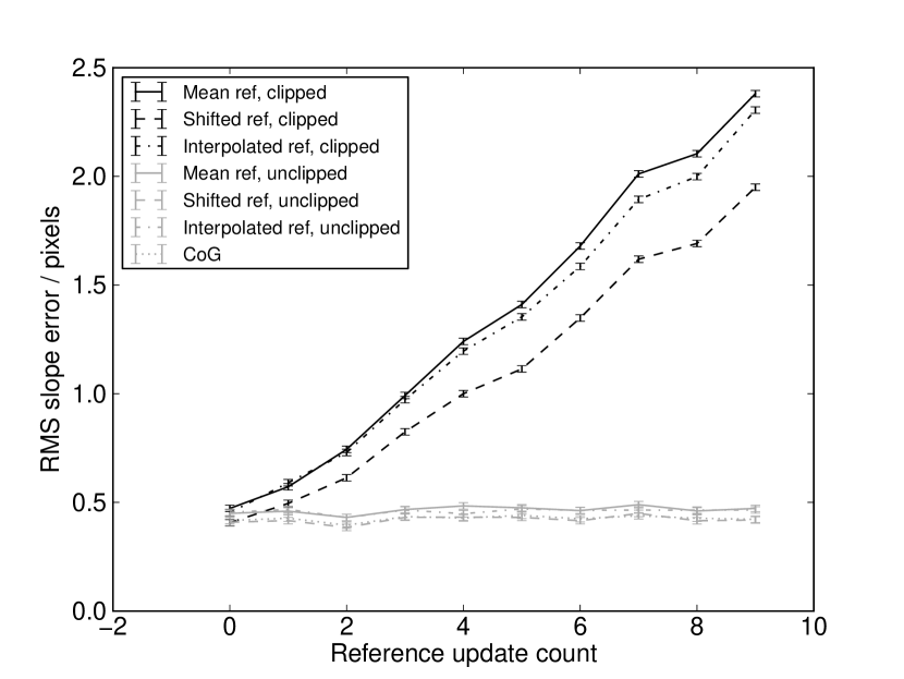
Figure 14: A figure showing the error in slope measurements due to build up of bias in reference slopes when incorrect clipping is used. Here, the x-axis represents the number of times the reference image and slopes have been updated. The “clipped” results (black curves) show the bias introduced by incorrect clipping, while the grey curves show that it is possible to continue updating the references without affecting performance.

4 Conclusions

We have presented a technique that allows correlation reference images to be updated in real-time for astronomical AO systems, whilst the AO loop is closed, without affecting the science PSF. This is of particular interest for systems with LGSs, where spot patterns show large amounts of elongation along one axis. This technique has been demonstrated successfully on-sky using the CANARY AO demonstrator instrument. We have investigated techniques to improve the accuracy of wavefront slope estimation related to the computation of the image correlations, using a Monte-Carlo AO simulation tool interfaced to a real-time control system. We recommend that of order 100 calibrated image frames are used for computation of the correlation reference, and that these images should be calibrated using a brightest pixel selection technique. Our results show that there is little difference between the three techniques investigated for reference image computation and therefore recommend that the shift-and-add method should be used since it performs well in most situations. We have also shown that these correlation based algorithms are more accurate than a centre-of-gravity algorithm in low and moderate signal-to-noise ratio regimes. We have not investigated truncation effects, always assuming that our elongated spots fit within the sub-aperture field of view, though we will study this in a future paper.

References

- Babcock (1953) Babcock H. W., 1953, Pub. Astron. Soc. Pacific, 65, 229
- Basden et al. (2010) Basden A., Geng D., Myers R., Younger E., 2010, Appl. Optics, 49, 6354
- Basden et al. (2010) Basden A., Myers R., Butterley T., 2010, Appl. Optics, 49, G1
- Basden (2014) Basden A. G., 2014, In press
- Basden et al. (2013) Basden A. G., Bharmal N. A., Myers R. M., Morris S. L., Morris T. J., 2013, MNRAS, 435, 992
- Basden et al. (2007) Basden A. G., Butterley T., Myers R. M., Wilson R. W., 2007, Appl. Optics, 46, 1089
- Basden & Myers (2012) Basden A. G., Myers R. M., 2012, MNRAS, 424, 1483
- Basden et al. (2012) Basden A. G., Myers R. M., Gendron E., 2012, MNRAS, 419, 1628
- Butler et al. (2003) Butler D. J., Davies R. I., Redfern R. M., Ageorges N., Fews H., 2003, A&A, 403, 775
- Davis et al. (2006) Davis D. S., Hickson P., Herriot G., She C.-Y., 2006, Optics Letters, 31, 3369
- Foy & Labeyrie (1985) Foy R., Labeyrie A., 1985, A&A, 152, L29
- Gendron et al. (2011) Gendron E., Vidal F., Brangier M., Morris T., Hubert Z., Basden A., Rousset G., Myers R., 2011, A&A, 529, L2
- Richards (2012) Richards K., 2012, in Society of Photo-Optical Instrumentation Engineers (SPIE) Conference Series Vol. 8447 of Society of Photo-Optical Instrumentation Engineers (SPIE) Conference Series, Adaptive optics real time processing design for the advanced technology solar telescope
- Shack (1971) Shack R. V., 1971, Journal of the Optical Society of America, 61, 656
- Thomas et al. (2006) Thomas S., Fusco T., Tokovinin A., Nicolle M., Michau V., Rousset G., 2006, MNRAS, 371, 323
- Thompson & Castle (1992) Thompson L. A., Castle R. M., 1992, Optics Letters, 17, 1485