Microlens Masses From Astrometry and Parallax in Space-Based Surveys: From Planets to Black Holes

Abstract

We show that space-based microlensing experiments can recover lens masses and distances for a large fraction of all events (those with individual photometric errors $\lesssim 0.01\,$mag) using a combination of one-dimensional microlens parallaxes and astrometric microlensing. This will provide a powerful probe of the mass distributions of planets, black holes, and neutron stars, the distribution of planets as a function of Galactic environment, and the velocity distributions of black holes and neutron stars. While systematics are in principle a significant concern, we show that it is possible to vet against all systematics (known and unknown) using single-epoch precursor observations with the Hubble Space Telescope roughly 10 years before the space mission.

1 Introduction

At present, well under 1% of microlensing events yield mass and distance measurements. It is estimated, for example, that 0.8% of all events (i.e., roughly 20 per year) are due to isolated black holes (Gould, 2000), but to date not a single one of these has been reliably identified as such. Microlensing planet searches yield a dozen detections per year, a figure likely to increase several fold over the next few years. These planets are distributed along the line of sight from near the Solar circle to the Galactic bulge, and so potentially could tell us about planet frequency as a function of Galactic environment. In fact, distances to these planets are mostly unknown, and those with measured distances are highly biased toward being nearby. Microlensing mass and distance measurements could yield mass functions and velocity distributions of black holes and neutron stars, find detailed structures in the mass distribution of planets, identify hosts by stellar type, and much more.

The main difficulty is that microlensing events routinely return only one parameter that is sensitive to the mass and distance, namely the Einstein timescale,

$$t_{\rm E}={\theta_{\rm E}\over\mu_{\rm rel}};\quad\theta_{\rm E}=\sqrt{\kappa M\pi_{\rm rel}}\simeq 0.3\,{\rm mas}\sqrt{{M\over 0.5\,M_{\odot}}\,{\pi_{\rm rel}\over 20{\mu\rm as}}};\quad\kappa\equiv{4G\over c^{2}\,{\rm AU}}\simeq 8.1\,{{\rm mas}\over M_{\odot}}.$$ (1)

Here $M$ is the lens mass, $\theta_{\rm E}$ is the Einstein radius, $\pi_{\rm rel}$ is the lens-source relative parallax, and $\mu_{\rm rel}$ is the lens-source relative proper motion in the frame of the observer (usually on Earth: $\mu_{\rm rel}=\mu_{\rm geo}$) at the peak of the event.

To disentangle the three physical parameters ($M,\pi_{\rm rel},\mu_{\rm rel}$) that enter $t_{\rm E}$ clearly requires two additional observables. For dark (or otherwise undetectable) lenses, these must be the Einstein radius $\theta_{\rm E}$ and the amplitude of the microlens parallax vector, $\pi_{\rm E}=|{\mbox{\boldmath$\pi$}}_{\rm E}|$. This amplitude is simply the trigonometric relative parallax scaled to the Einstein radius,

$$\pi_{\rm E}={\pi_{\rm rel}\over\theta_{\rm E}}.$$ (2)

The direction of ${\mbox{\boldmath$\pi$}}_{\rm E}$ is that of the lens-source relative motion, ${\mbox{\boldmath$\pi$}}_{\rm E}/\pi_{\rm E}={\mbox{\boldmath$\mu$}}_{\rm rel}/\mu_{\rm rel}$.

The usual path to measuring the lens mass and distance in the very few cases that this has been done is to combine measurements of $\theta_{\rm E}$ and the vector ${\mbox{\boldmath$\pi$}}_{\rm E}$

$$(\theta_{\rm E}\,\oplus\,{\mbox{\boldmath$\pi$}}_{\rm E})\Rightarrow M={\theta_{\rm E}\over\kappa\pi_{\rm E}}\quad\oplus\quad\pi_{\rm rel}=\theta_{\rm E}\pi_{\rm E}\qquad{\rm(traditional)}.$$ (3)

Since the source parallax $\pi_{s}$ is usually well known (typical uncertainty $\lesssim 10\,{\mu\rm as}$), measuring $\pi_{\rm rel}$ is equivalent to measuring the lens distance $D_{l}={\rm AU}/(\pi_{\rm rel}+\pi_{s})$.

In this approach, $\theta_{\rm E}$ is only measurable for the subset of events in which the source comes close to a caustic structure (typically caused by a planetary or binary system). The lightcurve then yields $\rho=\theta_{*}/\theta_{\rm E}$, i.e., the ratio of the angular source radius to the Einstein radius. Since $\theta_{*}$ can be determined from the source color and brightness (Yoo et al., 2004), one can then measure $\theta_{\rm E}=\theta_{*}/\rho$. Relatively few events have such caustic anomalies. Fortunately, this subset includes most planetary events. However, it includes extremely few black holes or neutron stars.

This latter fact is unfortunate because massive objects are the most susceptible to microlens parallax measurements, which are the other necessary ingredient. The microlens parallax $\pi_{\rm E}=\pi_{\rm rel}/\theta_{\rm E}$ specifies the amplitude of lens-source relative displacement due to reflex motion of the observer (typically on Earth) normalized to the Einstein radius. If microlensing events lasted a year, this would induce very obvious annual oscillations in the lightcurve. But since most events are much shorter, they contain only a fraction of an oscillation, which is usually not detectable. Even when detectable, it is usually only possible to measure one component of the parallax vector,

$$\pi_{{\rm E},\parallel}\equiv{\mbox{\boldmath$\pi$}}_{\rm E}\cdot\hat{\bf n}_{a},$$ (4)

the component in the direction $\hat{\bf n}_{a}$ of the observer’s instantaneous acceleration (toward the projected position of the Sun) at the peak of the event. To the degree that $\hat{\bf n}_{a}$ is aligned with ${\mbox{\boldmath$\mu$}}_{\rm rel}$, the event becomes asymmetric, rising either faster or slower than it falls. Since microlensing events are intrinsically symmetric, asymmetric deviations are easily detected. On the other hand, to the extent that ${\mbox{\boldmath$\mu$}}_{\rm rel}$ is perpendicular to $\hat{\bf n}_{a}$, there is a symmetric distortion, which easily masquerades as small changes in other symmetric parameters.

Clearly, ${\mbox{\boldmath$\pi$}}_{\rm E}$ is easiest to measure when it is large and/or when the timescale of the event is longer. For example, massive objects typically generate longer events, so there is more chance to measure the full parallax effect. In practice, mass and distance measurements are mainly made for binary and planetary events (yielding $\theta_{\rm E}$) that happen to be relatively close (so large $\pi_{\rm rel}$, implying large, more easily measurable ${\mbox{\boldmath$\pi$}}_{\rm E}$).

Here we propose an alternate route to microlens mass measurements. To do so, we introduce a new microlensing quantity, the vector Einstein radius ${\mbox{\boldmath$\theta$}}_{\rm E}$

$${\mbox{\boldmath$\theta$}}_{\rm E}\equiv{\mbox{\boldmath$\mu$}}_{\rm rel}t_{\rm E};\qquad\theta_{{\rm E},\parallel}\equiv{\mbox{\boldmath$\theta$}}_{\rm E}\cdot\hat{\bf n}_{a}.$$ (5)

We show that this new quantity is the observable in astrometric microlensing and that it leads to a new path to microlens mass and distance measurements:

$$({\mbox{\boldmath$\theta$}}_{\rm E}\,\oplus\,\pi_{{\rm E},\parallel})\Rightarrow M={\theta_{{\rm E},\parallel}\over\kappa\pi_{{\rm E},\parallel}}\quad\oplus\quad\pi_{\rm rel}=\theta_{\rm E}^{2}{\pi_{{\rm E},\parallel}\over\theta_{{\rm E},\parallel}}\qquad{\rm(new)}.$$ (6)

In Section 2, we review astrometric microlensing and show that what it actually measures is ${\mbox{\boldmath$\theta$}}_{\rm E}$. In Sections 3 and 4, we demonstrate that both ${\mbox{\boldmath$\theta$}}_{\rm E}$ and $\pi_{{\rm E},\parallel}$ can be measured for a large fraction of events detected in space-based microlensing surveys. In Section 5, we quantitatively evaluate problems posed by the known unknowns of this approach, and in Section 6 we discuss the unknown unknowns. The latter appear particularly intractable, but in Section 7 we present an empirical method to control the unknowns, both known and unknown.

2 Review of Astrometric Microlensing

Microlenses split source light into 2 or more images that are separated on the sky by angles of order $\theta_{\rm E}$, which is typically $\lesssim 1\,$mas. Hence, these images are not typically resolved. However, the centroid of the combined image light is displaced from the source position by an amount that scales directly as $\theta_{\rm E}$, and hence it is in principle possible to measure $\theta_{\rm E}$ from a time series of astrometric measurements (Miyamoto & Yoshii, 1995; Hog et al., 1995; Walker, 1995).

For a point lens, there are two images with positions relative to the lens $\Delta{\mbox{\boldmath$\theta$}}_{\pm}$ and magnifications $A_{\pm}$ given by (Einstein, 1936)

$$\Delta{\mbox{\boldmath$\theta$}}_{\pm}={u\pm\sqrt{u^{2}+4}\over 2}{\Delta{\mbox{\boldmath$\theta$}}\over u};\qquad{\bf u}\equiv{\Delta{\mbox{\boldmath$\theta$}}\over\theta_{\rm E}};\qquad\Delta{\mbox{\boldmath$\theta$}}\equiv{\mbox{\boldmath$\theta$}}_{s}-{\mbox{\boldmath$\theta$}}_{l},$$ (7)

$$A_{\pm}={A\pm 1\over 2},\qquad A={u^{2}+2\over u(u^{2}+4)^{1/2}},$$ (8)

where ${\mbox{\boldmath$\theta$}}_{s}$ and ${\mbox{\boldmath$\theta$}}_{l}$ are the astrometric positions of the source and lens.

Therefore, the displacement of the image centroid from the source is

$$\Delta{\mbox{\boldmath$\theta$}}_{\rm cen}={A_{+}\Delta{\mbox{\boldmath$\theta$}}_{+}+A_{-}\Delta{\mbox{\boldmath$\theta$}}_{-}\over A}-\Delta{\mbox{\boldmath$\theta$}}={\Delta{\mbox{\boldmath$\theta$}}\over u^{2}+2}={{\bf u}\over u^{2}+2}\theta_{\rm E}$$ (9)

If the lens-source relative motion is approximated as uniform

$$\Delta{\mbox{\boldmath$\theta$}}(t)=(t-t_{0}){\mbox{\boldmath$\mu$}}_{\rm rel}+{\mbox{\boldmath$\beta$}}\theta_{\rm E}$$ (10)

where $t_{0}$ is the time of closest approach and $\beta$ is the normalized impact parameter $({\mbox{\boldmath$\beta$}}\perp{\mbox{\boldmath$\mu$}}_{\rm rel})$, then $\Delta{\mbox{\boldmath$\theta$}}_{\rm cen}$ traces out an ellipse that is centered at $({\mbox{\boldmath$\beta$}}\theta_{\rm E}/2)/(\beta^{2}+2)$ and whose vector semi-major and semi-minor axes are

$${\bf a}={{\mbox{\boldmath$\theta$}}_{\rm E}\over 2(2+\beta^{2})^{1/2}};\qquad{\bf b}={{\mbox{\boldmath$\beta$}}\theta_{\rm E}\over 2(2+\beta^{2})}.$$ (11)

Equation (11) verifies the claim made in Section 1 that astrometric microlensing measures ${\mbox{\boldmath$\theta$}}_{\rm E}$. The axis ratio and eccentricity of this ellipse are

$${a\over b}=\sqrt{{2\over\beta^{2}}+1};\qquad e=\sqrt{2\over\beta^{2}+2}.$$ (12)

We note that the lens-source relative motion may not be rectilinear for two reasons. First, either the source or lens may be accelerated by a companion. Second, even if both are intrinsically unaccelerated, the ellipse will be distorted by parallax effects from the accelerated motion of the observer (Boden et al., 1998). We treat the first effect in Section 5. The second effect is always be present at some level and so must be included in formal fits. However, it is generally quite small and so can be ignored in the simplified treatment given here, which is aimed at evaluating the viability of the method.

3 Application to Space-Based Surveys

Space-based microlensing surveys have a number of advantages over ground-based, but the most critical from the present perspective is the smaller point spread function (PSF). This has three major implications. First, for sources above sky, the astrometric precision is given by

$$\sigma_{\rm ast}=\sigma_{\rm phot}{{\rm FWHM}\over(\ln 256)^{1/2}}$$ (13)

where $\sigma_{\rm phot}$ is the fractional photometric precision, FWHM is the full width at half maximum of the PSF, and where we have assumed a Gaussian PSF for definiteness (since the formula barely changes for other plausible PSFs). Since microlensing experimental design is governed by requirements of photometric precision, this equation automatically gives space a factor 5–10 advantage relative in astrometry relative to the ground due to smaller PSF. Second, for the class of events relevant for this approach, the sources are above sky from space, while most ground-based sources are below sky. Finally, in high-resolution space-based images, the source and lens are almost always isolated from all unrelated stars, i.e., all stars other than possible companions to these two stars. This both facilitates precision astrometry and immensely simplifies the analysis.

Nevertheless, despite the vastly improved astrometry from space, astrometric precision is still the limiting factor in mass measurements. We will show below that the astrometric requirements imply that $\sigma_{\rm phot}\lesssim 0.01$. This precision virtually guarantees that $\pi_{{\rm E},\parallel}$ will be well measured. For example, Figure 3 from Gould (2012) shows the error “ellipse” for parallax in a simulated microlensing event with a factor $\sim 2$ better precision than the typical one envisaged in this paper. We put “ellipse” in quotation marks because it is difficult to make out its width in the $\hat{\bf n}_{a}$ direction. We will therefore assume that $\pi_{{\rm E},\parallel}$ is measured much better than $\theta$. Note, from Equation (16) of Gould (2012), that $\pi_{{\rm E},\parallel}$ precision deteriorates for shorter timescale events $\propto t_{\rm E}^{-2}$. However, the shortest events are those for which astrometric effects are also extremely difficult to measure. Hence, while there may be some exceptions, it is reasonable to assume that whenever ${\mbox{\boldmath$\theta$}}_{\rm E}$ can be measured, $\pi_{{\rm E},\parallel}$ will have been measured better.

3.1 Astrometric Microlensing Precision

Similarly, but more so, for the events with high enough precision to enable astrometric measurements, the basic event parameters $(t_{0},\beta,t_{\rm E})$ will be known with essentially infinite precision. Therefore, the shape of the astrometric ellipse will likewise be known with essentially infinite precision from the photometric data (Equation (12)).

Thus, six parameters are required to describe the image-centroid trajectory in the neighborhood of the peak of the event: the vector Einstein radius ${\mbox{\boldmath$\theta$}}_{\rm E}$, the vector source proper motion ${\mbox{\boldmath$\mu$}}_{s}$, and the vector source position at the peak of the event ${\mbox{\boldmath$\theta$}}_{s,0}$. We will begin by approximating that ${\mbox{\boldmath$\mu$}}_{s}$ and ${\mbox{\boldmath$\theta$}}_{s,0}$ as known perfectly and test further below how well this holds and under what conditions.

Then each astrometric measurement $k$ contributes to the determination of the magnitude of $\theta_{\rm E}$ by

$$\sigma_{k}(\theta_{\rm E})=\sigma_{{\rm ast},k}{u_{k}^{2}+2\over u_{k}},$$ (14)

where $\sigma_{{\rm ast},k}$ is the astrometric precision of the measurement at separation $u_{k}$. If the source is above sky, and assuming photon-limited statistics, then $\sigma_{{\rm ast},k}=A_{k}^{-1/2}\sigma_{{\rm ast},0}$, where $\sigma_{{\rm ast},0}$ is the astrometric precision at baseline. Then for a uniform series of $N$ such measurements over a time interval $\Delta t=t_{2}-t_{1}$, the combined precision is

$$\sigma(\theta_{\rm E})=\sigma_{{\rm ast},0}\sqrt{\Delta\tau\over N}\biggl{[}\int_{t_{1}}^{t_{2}}d\tau G[u(\tau)]\biggr{]}^{-1/2},$$ (15)

where $\tau\equiv(t-t_{0})/t_{\rm E}$, $\Delta\tau=\Delta t/t_{\rm E}$ and

$$G(u)\equiv\biggl{(}{u\over u^{2}+2}\biggr{)}^{2}A(u)={u\over(u^{2}+2)\sqrt{u^{2}+4}}.$$ (16)

Similarly, the error in $\phi$, the angular orientation of ${\mbox{\boldmath$\theta$}}_{\rm E}$, is given by $\sigma(\phi)=\sigma(\theta_{\rm E})/\theta_{\rm E}$, so that

$$\sigma(\theta_{{\rm E},\parallel})=\sigma(\theta_{{\rm E},\perp})=\sigma(\theta_{\rm E}).$$ (17)

Explicitly,

$$\sigma(\theta_{\rm E})={\sigma_{{\rm ast},0}\over\sqrt{N\langle H\rangle}}\rightarrow 28\,{\mu\rm as}{\sigma_{{\rm phot},0}\over 0.01}\,{{\rm FWHM}\over 175\,{\rm mas}}\,\biggl{(}{N\over 7000}\biggr{)}^{-1/2}\biggl{(}{\langle H\rangle\over 0.1}\biggr{)}^{-1/2}$$ (18)

where

$$\langle H\rangle\equiv{\tau_{2}H(\tau_{2};\beta)-\tau_{1}H(\tau_{1};\beta)\over\tau_{2}-\tau_{1}};\qquad H(\tau;\beta)\equiv{1\over\tau}\int_{0}^{\tau}d\tau^{\prime}G[u(\tau^{\prime});\beta],$$ (19)

and $H(-\tau;\beta)=H(\tau;\beta)$. It is important to note that $\sigma(\theta_{\rm E})$ is larger than the combined astrometric precision $N^{-1/2}\sigma_{\rm ast,0}$ by $\langle H\rangle^{-1/2}$ because the astrometric offset that is being measured is smaller than $\theta_{\rm E}$ by this factor. Hence, when comparing systematic to statistical errors, it is the latter quantity $N^{-1/2}\sigma_{\rm ast,0}=\sigma(\theta_{\rm E})\langle H\rangle^{-1/2}\rightarrow 9\,{\mu\rm as}$ that must be considered.

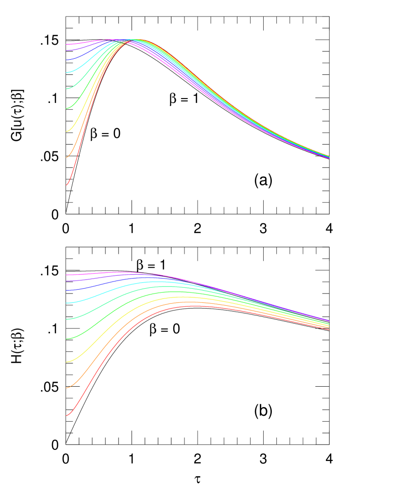
Figure 1: Function $G$ and its integral $H$, whose expressions are given explicitly by Equations (16) and (19). As shown by Equation (18) the error in ${\mbox{\boldmath$\theta$}}_{\rm E}$ scales as $\langle H\rangle^{-1/2}$, which according to Equation (19) is similar to $[H({\rm few},\beta)]^{-1/2}\sim 3$ for typical events.

Figure 1 shows the function $G[u(\tau);\beta]$ and $H(\tau;\beta)$ for 11 values of $\beta$, $0\leq\beta\leq 1$. It shows that for a very broad range of conditions, $\langle H\rangle\sim 0.1$. Moreover, since this quantity enters Equation (18) only as the square root, the astrometric precision is approximately independent of impact parameter $\beta$, timescale $t_{\rm E}$, and time of closest approach $t_{0}$ over this broad range (provided that the peak is within or near the interval of observations). That is, under the assumption of photon-limited measurements, the indicated precision of $28\,{\mu\rm as}$ can typically be achieved under the fiducial conditions, $N=7000$, ${\rm FWHM}=175\,{\rm mas}$, and $\sigma_{{\rm phot},0}=1\%$.

These conditions have been scaled to one version of observations of the proposed WFIRST satellite, i.e., 94 observations per day of each of 10 fields, over a continuous $\Delta t=72\,$day interval. Simulations by M. Penny (2013, private communication), show that approximately half of the events with detectable Earth-mass planets would have $\sigma_{{\rm phot},0}<1\%$. From Equation (1), typically $\theta_{\rm E}\sim 0.3\,{\rm mas}$. Such events would yield 10-sigma detections, i.e., 10% measurements of $\theta_{\rm E}$ under fiducial conditions. Of course, what is required for mass determinations is a measurement of $\theta_{{\rm E},\parallel}$, and this quantity is smaller than $\theta_{\rm E}$ by the cosine of some random angle. Nevertheless, this cosine will be $>0.5$ in 67% of all cases. Hence, Equation (18) implies that astrometric mass measurements are possible in a large fraction of cases.

Before continuing, we note that for $\tau\gtrsim 4$, all the curves in Figure 1b tend toward $H(\tau;0)$, which can be evaluated in closed form,

$$H(\tau,0)={1\over\sqrt{2}\tau}\ln{(\sqrt{\tau^{2}+4}-\sqrt{2})(1+\sqrt{2})\over\sqrt{\tau^{2}+2}}\rightarrow{0.62\over\tau}.$$ (20)

4 Known Knowns

4.1 Uncertainty in ${\mbox{\boldmath$\theta$}}_{s}$

In Section 3, we evaluated the precision of the ${\mbox{\boldmath$\theta$}}_{\rm E}$ measurement under the assumption that the true position of the source ${\mbox{\boldmath$\theta$}}_{s}={\mbox{\boldmath$\theta$}}_{s,0}+{\mbox{\boldmath$\mu$}}_{s}(t-t_{0})$ was known with infinite precision, so that the measurement (and measurement error) of its apparent position ${\mbox{\boldmath$\theta$}}_{\rm cen}$ directly gave the offset between these, $\Delta{\mbox{\boldmath$\theta$}}_{\rm cen}={\mbox{\boldmath$\theta$}}_{\rm cen}-{\mbox{\boldmath$\theta$}}_{s}$. In fact, ${\mbox{\boldmath$\theta$}}_{s}$ must itself be determined from astrometric measurements, which of course have similar individual precisions to those of the ${\mbox{\boldmath$\theta$}}_{\rm cen}$ measurements. Therefore, it is far from obvious that the error in ${\mbox{\boldmath$\theta$}}_{s}$ can be ignored.

We address this issue in several phases. We first assume that the lens is dark and that the source is isolated, i.e., that it has no massive companions and so is moving in rectilinear relative motion. Hence, the four required parameters ${\mbox{\boldmath$\theta$}}_{s,0}$ and ${\mbox{\boldmath$\mu$}}_{s}$ can be determined from a linear fit to data away from the event. In practice, of course, one would fit all the data to a model with all the parameters. However, to determine the precision of these four parameters, we can idealize the epochs in years other than the event as unaffected by the event. We further idealize all the observations during each year as taking place at the same time. Assuming there are $n+1$ years of observations (labeled $0,1,\ldots n$) with the event in the $j$th year, then the inverse covariance matrix of each directional-component of the pair (${\mbox{\boldmath$\theta$}}_{s,0},{\mbox{\boldmath$\mu$}}_{s}$) is given by (e.g., Gould 2003)

$$C^{-1}={N\over 6\sigma_{{\rm ast},0}^{2}}\left(\matrix{6n&3(n+1)(n-2j){\rm yr}\cr 3(n+1)(n-2j){\rm yr}&(n+1)[n(2n+1)-6j(n-j)]{\rm yr}^{2}\cr}\right),$$ (21)

with e.g., $C_{11}^{1/2}=\sigma(\theta_{s,0,x})=\sigma(\theta_{s,0,y})$. For simplicity, we restrict consideration to the least ($j=0$ or $j=n$) and most $(j=n/2)$ favorable cases. The first point to note is that the error in the zero point dominates over the proper motion in either case

$${\sigma_{\mu}\over\sigma_{\theta}}=\sqrt{6\over(n+1)(2n+1)}{\rm yr}^{-1}\quad(j=0);\qquad{\sigma_{\mu}\over\sigma_{\theta}}=\sqrt{12\over(n+1)(n+2)}{\rm yr}^{-1}\quad(j=n/2).$$ (22)

That is, considering that for typical $n\sim 4$, these ratios are $<{\rm yr}^{-1}$, and that the source position needs to be known for a time $\Delta t<0.2\,{\rm yr}$, the proper motion errors enter at an order of magnitude lower level than the positional errors. These positional errors can then be directly compared to the errors in the mean offset estimated above, i.e., $\theta_{\rm E}\langle H\rangle^{1/2}$:

$${\sigma(\theta_{s,0})\over\sigma(\theta_{\rm E})\langle H\rangle^{1/2}}=\sqrt{2(n+1)\over n(n-1)}\quad(j=0);\qquad{\sigma(\theta_{s,0})\over\sigma(\theta_{\rm E})\langle H\rangle^{1/2}}=\sqrt{1\over n}.\quad(j=n/2).$$ (23)

For example, for $n=4$, these ratios are 90% and 50%, respectively. Given that these errors enter in quadrature, the second is sub-dominant but the first can be important. Note, however, that for events whose peak is very roughly near the center of a given year’s observations, the role of the uncertainty in the source position is greatly reduced by the symmetry in the time evolution of the offset along the direction of motion, ${\mbox{\boldmath$\mu$}}_{\rm rel}$.

4.2 Luminous Lens

If the lens is luminous, then the astrometric measurements at times away from the event will yield the position and proper motion of the combined lens and source light. When these are projected back to $t_{0}$, they will yield the lens-source centroid (as it would appear if there were no astrometric lensing), with the same precision. The division between lens and source light will be known very precisely (under the assumption that neither has a companion) because the microlensing fit precisely gives the source flux, and this can be subtracted from the baseline flux to give the lens flux.

The main potential problem is that the amplitude of the astrometric signal will be degraded because the source undergoes an astrometric deviation but the blended light from the lens does not. Han & Jeong (1999) show that the combined light of the lens and source follows a nearly-elliptical path, which is less eccentric than the trajectory of the combined source images by themselves. They conjecture that this shape is truly an ellipse, although this has not to our knowledge yet been proved.

However, if the lens is relatively faint, then this degradation is minor and, as indicated above, with known functional form. And if the lens is bright, then its mass and distance can be estimated photometrically, so that the astrometric microlensing information is relatively unimportant.

5 Known Unknowns

It is known that stars in general frequently have binary companions, but it is unknown a priori whether this is the case for the particular lens and source in an event being studied. Since such companions can affect the interpretation of astrometric data, we classify them as “known unknowns”.

We consider first companions to the source. The typical sources with sufficient S/N for astrometric measurements are G dwarfs, and for these the companion is typically so much fainter than the primary (Duquennoy & Mayor, 1991) that it can usually be considered “dark”. Accelerated source motion due to such companions is usually called “xallarap” in the context of photometric microlensing and we retain that terminology here. The main concern is that this xallarap effect would go unrecognized and would subtly corrupt the interpolation or extrapolation of the source position back to the time of the event. For simplicity, we consider a face-on circular orbit. If the period is $P<5\,\rm yr$ (typical duration of a space mission), then the amplitude of the astrometric signature due to the companion will be simply

$$\Delta\theta_{\rm bin}=30\,{\mu\rm as}\,\biggl{(}{P\over{\rm yr}}\biggr{)}^{2/3}\biggl{(}{M+m\over M_{\odot}}\biggr{)}^{1/3}\biggl{(}{m/(M+m)\over 1/4}\biggr{)}\biggl{(}{D_{s}\over{\rm 8\,kpc}}\biggr{)}^{-1}.$$ (24)

Since the fiducial year-as-epoch astrometric error is about $9\,{\mu\rm as}$, this implies that all such companions would be directly detectable unless they had periods smaller than one year and/or had exceptionally low-mass. At shorter periods $P\lesssim 1\,$yr, the astrometric signature would not, by itself, be secure. However, such close companions typically give rise to a photometric xallarap signature, even in ground-based data (e.g., Poindexter et al. 2005), and the low-level astrometric signature could be combined with photometric data to securely identify the xallarap signature.

Let us then consider the opposite limit, in which the period is much longer than the mission, so that the astrometric effect can be approximated as uniform acceleration,

$$\alpha=16\,{\mu\rm as}\,{\rm yr}^{-2}\biggl{(}{m\over(1/3)M_{\odot}}\biggr{)}\biggl{(}{a\over 10\,{\rm AU}}\biggr{)}^{-2}\biggl{(}{D_{s}\over{\rm 8\,kpc}}\biggr{)}^{-1}\sin\phi,$$ (25)

where $a$ is the physical separation and $\phi$ is the angle relative to the line of sight. At, for example, $a\sim 10\,{\rm AU}$, this signal is too small to be reliably identified. However, if it is simply ignored, this will lead to an incorrect estimate of ${\mbox{\boldmath$\theta$}}_{s,0}$ in the direction of acceleration by

$$|\Delta{\mbox{\boldmath$\theta$}}_{s,0}|={(n+1)(n+2)\over 12}\alpha\,{\rm yr}^{2}\quad(j=0);\qquad|\Delta{\mbox{\boldmath$\theta$}}_{s,0}|={(n+1)(n+2)\over 24}\alpha\,{\rm yr}^{2}\quad(j=n/2).$$ (26)

To estimate the impact of these systematic errors, they should be compared to the $\sigma(\theta_{\rm E})\langle H\rangle^{1/2}\sim 10\,{\mu\rm as}$ statistical error. Hence the systematics can be significant, but only for about 0.5 dex of separations ($5\,{\rm AU}\lesssim a\lesssim 15\,{\rm AU}$), i.e., a few percent of all sources. We return to the problem of evaluating the impact of such systematic errors in Section 7.

Note that even if the source companion is extremely faint, it could significantly displace the centroid of light if it were sufficiently far away, thereby acting with a big “lever arm”. For example, a companion that lay projected at 500 AU and was 1/500 of the source brightness would displace the centroid by $125\,{\mu\rm as}$ which is quite substantial compared to the quantities being measured. However, this has no impact because this displacement is essentially identical for all measurements and so does not affect the differential astrometry, which is the basis of the astrometric microlensing measurement.

We now turn to companions to the lens. Just as with source companions, the steepness of the mass-luminosity relation ensures that in most cases the companion will have very different brightness from the lens. However, in contrast to the source case, the lens companion is almost as likely to be brighter than the lens as fainter. This is because microlensing event detection strongly selects on source brightness, but it is essentially indifferent to lens brightness per se. Therefore, the only selection effect is the relative Einstein radii, which favors the heavier of two well-separated companions by the square root of their mass ratio. The heavier of the two stars is usually also brighter, but the (square root of the) mass ratio is typically tiny compared to the luminosity ratio. Even if the companion is brighter, this does not necessarily mean that its light will be detectable. However, it does mean that in a substantial minority of all cases in which excess light is detected, this excess will be due to a lens companion and not the lens. Nevertheless in the great majority of these cases, the lens companion can be identified using the method of Batista et al. (2013) wherein one measures the astrometric offset of the source at the peak of the event (determined from difference imaging) relative to the baseline source. While the exact precision of this measurement depends on the peak magnification and event timescale, typically the precision will be of order $20\,{\mu\rm as}$ for data of sufficient quality to do astrometric microlensing. Even if the companion is just 10% of the source brightness, this implies that it will be detectable if it lies more than a few AU from the lens. In the remaining cases, the companion will lie inside (or at least very near) the Einstein radius of the lens and therefore will give rise to pronounced astrometric effects that will be of interest to measure (Han et al., 1999; Han, 2001; Gould & Han, 2000). It will also very likely give rise to photometric (binary lensing) effects.

6 Unknown Unknowns

Even very small systematic errors could in principle radically undermine the mass determinations derived from astrometric microlensing. The precision of the masses relies on “root-n” scaling of the statistical error bars in which $n\sim 10^{8}$ photons (i.e. $N\sim 7000\,{\rm yr}^{-1}$ observations each with ${\rm(S/N)^{2}}\sim 10^{4}$). However, systematic errors do not scale this way. As an example, if the mean of the astrometric reference frame were displaced from the source by just $1^{\prime\prime}$, the differential aberration of light would be ${\cal O}(10\,{\mu\rm as})$. Of course, one does not expect differential aberration to be ignored in the analysis, but the point is that other very tiny effects in the optics, the detector, etc., could impact the result. Happily, in the next section, we discuss ways to control for systematic errors of the most general sort.

7 Systematic Vetting of Unknowns (Known and Unknown)

Given that these mass measurements will be both near the detection limit and dependent on near-perfect scaling of root-n errors, the only method for assessing their viability is to make independent proper motion measurements of a substantial subsample. At first sight this appears to be a daunting task because the whole driver of the approach we have outlined is to measure the masses of objects that are otherwise unmeasurable. However, as mentioned in the Introduction, there is already a widely used technique for measuring the scalar proper motion $\mu_{\rm geo}$ for events with caustic crossings, which includes most planetary and binary events. These are also among the events of greatest direct interest.

Of course, as we have emphasized, the mass determinations discussed here require measurement of the vector proper motion ${\mbox{\boldmath$\mu$}}_{\rm geo}$, not just its amplitude. However, if the amplitudes were correctly estimated from astrometric microlensing (within errors) it would be strong evidence that the directions were measured correctly as well, since the amplitude and direction are approximately independent and derive from the same quality of data. This provides one check on the astrometric proper motion measurements.

Nevertheless, from the discussion in Section 5, it is guaranteed that systematics will corrupt at least some measurements and, as emphasized in Section 6 the level of this problem is very difficult to assess in advance. Therefore, it would be valuable to have independent measurements of the vector proper motions (and for a much larger subsample than the scalar proper motions discussed above) in order to be able to systematically study the conditions under which the astrometric measurements are significantly corrupted and, hopefully, to identify the source of these problems and find means to ameliorate them.

This can be accomplished via a high-resolution survey of future microlensing fields using the Hubble Space Telescope (HST). In a subset of cases that we identify below, the future lens and source will be separately resolved in such images. Since the precise time of their near-perfect future alignment will be determined by the microlensing event, it will be possible to measure their heliocentric proper motion ${\mbox{\boldmath$\mu$}}_{\rm hel}$. This is related to their geocentric motion by

$${\mbox{\boldmath$\mu$}}_{\rm hel}={\mbox{\boldmath$\mu$}}_{\rm geo}+{{\bf v}_{\oplus,\perp}\over{\rm AU}}\pi_{\rm rel}$$ (27)

where ${\bf v}_{\oplus,\perp}$ is the motion of Earth relative to the Sun projected on the plane of the sky at the peak of the event, which is known extremely well. Note that $\pi_{\rm rel}$ can be estimated either by photometric parallax of the separately resolved lens or from the overall microlensing solution: $\pi_{\rm rel}=\theta_{\rm E}\pi_{\rm E}$.

There are several challenges to making such measurements. First, of course, to be separately resolved the lens must be luminous. This already precludes using this test on dark lenses. However, as we have argued above, if the lens is a factor several fainter than the source, the astrometric measurements are only mildly affected and in a well-understood way. Hence the approach could plausibly be applied to lenses that are a factor $\sim 3$ to $\sim 20$ fainter than the source.

More challenging, the lens and source must be separately resolved at the time of the earlier observations. This requirement will vary as a function of system parameters, but for definiteness, we adopt the FWHM as the minimum separation. This immediately leads to the proper motion requirement

$$\mu_{\rm hel}>\mu_{\rm min}={{\rm FWHM}\over\Delta t}=8.4\,{\rm mas}\,{\rm yr}^{-1}{\lambda\over 0.8\,\mu{\rm m}}\biggl{(}{\Delta t\over 10\,{\rm yr}}\biggr{)}^{-1},$$ (28)

where $\lambda$ is the central wavelength of the observing passband and $\Delta t$ is the elapsed time between the HST observations and the microlensing event. Note that this minimum is substantially higher than the typical $\mu_{\rm geo}$ measured for microlensing events (Henderson et al., 2014).

While at first sight one might think that these advance HST observations should be done in a similar passband to the microlensing observations, Equation (28) makes clear that there is a huge premium on going to shorter wavelengths. In particular, if we consider bulge lenses and assume isotropic bulge-star proper motion dispersions $\sigma_{\mu}\ll\mu_{\rm min}$, then the fraction of events satisfying Equation (28) is just

$$f={2\over\sqrt{\pi}}x\exp(-x^{2})\qquad\biggl{(}x\equiv{\mu_{\rm min}\over 2\sigma_{\mu}}\biggr{)}.$$ (29)

If we then adopt $\sigma_{\mu}=3\,{\rm mas}\,{\rm yr}^{-1}$, $\Delta t=10\,$yr, and $\lambda=\lambda_{I}=0.8\,\mu$m, then $f=22\%$. But for the same assumptions and $\lambda=\lambda_{H}=1.65\,\mu$m, $f<0.1\%$. Fortunately, however, initial work by M. Penny (2013, private communication) shows that the best WFIRST fields have significant (roughly 50%) overlap with current OGLE fields where the extinction is low enough that many microlensing events are currently being found in $I$-band. On the other hand, the several additional magnitudes of extinction in $V$ band preclude going to substantially shorter wavelengths. Therefore, early observations of these overlapping OGLE and WFIRST fields should be carried out in $I$ band.

References

- Batista et al. (2013) Batista, V., Beaulieu, J.-P., Gould, A., Bennett, D.P., Yee, J.C., Fukui, A., Sumi, T., & Udalski, A. 2014, ApJ, 780, 54
- Boden et al. (1998) Boden, A.F., Shao, M., & van Buren, D. ApJ, 502, 538
- Choi et al. (2013) Choi, J.-Y., Han, C., Udalski, A., et al. 2013, ApJ, 768, 129
- Dong et al. (2007) Dong, S., Udalski, A., Gould, A., et al. 2007, ApJ, 664,862
- Duquennoy & Mayor (1991) Duquennoy, A. & Mayor, M. 1991, A&A, 248 485
- Einstein (1936) Einstein, A. 1936, Science, 84, 506
- Gaudi & Gould (1997) Gaudi, B.S. & Gould, A. 1997, ApJ, 477, 152
- Gould (1992) Gould, A. 1992, ApJ, 392, 442
- Gould (1994) Gould, A. 1994, ApJ, 421, L75
- Gould (1995) Gould, A. 1995, ApJ, 441, L21
- Gould (1997) Gould, A. 1997, ApJ, 480, 188
- Gould (1999) Gould, A. 1999, ApJ, 514, 869
- Gould (2000) Gould, A. 2000, ApJ, 535, 928
- Gould (2003) Gould, A. 2003, arXiv:astro-ph/0310577
- Gould (2004) Gould, A. 2004, ApJ, 606, 319
- Gould (2012) Gould, A. 2012, ApJ, 763, L35
- Gould & Han (2000) Gould, A. & Han, C. 2000, ApJ, 538, 653
- Gould & Yee (2013) Gould, A. & Yee, J.C. 2013, ApJ, 767, 42
- Han (2001) Han, C. 2001, MNRAS, 325, 1281
- Han & Jeong (1999) Han, C. & Jeong, Y. 1999, MNRAS, 309, 404
- Han et al. (1999) Han, C. Chun, M.-S. & Chang, K. 1999, ApJ, 526, 405
- Henderson et al. (2014) Henderson, C.B., Park, H., Sumi, T. et al. 2014, in preparation
- Hog et al. (1995) Hog, E., Novikov, I.D., & Polanarev, A.G. 1995, A&A, 294, 287
- Miyamoto & Yoshii (1995) Miyamoto, M. & Yoshii, Y. 1995, AJ, 110, 1427
- Poindexter et al. (2005) Poindexter, S., Afonso, C., Bennett, D.P., Glicenstein, J.-F., Gould, A, Szymański, M.K., & Udalski, A. 2005, ApJ, 633, 914
- Refsdal (1966) Refsdal, S. 1966, MNRAS, 134, 315
- Shin et al. (2011) Shin, I.-G., Udalski, A., Han, C. et al. 2011, ApJ, 735, 85
- Shin et al. (2012) Shin, I.-G., Han, C., Choi, J.-Y. et al. 2012, ApJ, 755, 91
- Walker (1995) Walker, M.A. 1995, ApJ, 453, 37
- Yee et al. (2012) Yee, J.C., Shvartzwald, Y., Gal-Yam, A., et al. 2012, ApJ, 755, 102
- Yoo et al. (2004) Yoo, J., et al. 2004, ApJ, 603, 139