Acceleration feature points of unsteady shear flows

Abstract

In this paper, we propose a novel framework to extract features such as vortex cores and saddle points in two-dimensional unsteady flows. This feature extraction strategy generalizes critical points of snapshot topology in a Galilean-invariant manner, allows to prioritize features according to their strength and longevity, enables to track the temporal evolution of features, is robust against noise and has no subjective parameters. These characteristics are realized via several constitutive elements. First, acceleration is employed as a feature identifier following Goto and Vassilicos (2006), thus ensuring Galilean invariance. Second, the acceleration magnitude is used as basis for a mathematically well-developed scalar field topology. The minima of this field are called acceleration feature points, a superset of the acceleration zeros. These points are discriminated into vortices and saddle points depending the spectral properties of the velocity Jacobian. Third, all operations are based on discrete topology for the scalar field with combinatorial algorithms. This parameter-free foundation allows (1) to use persistence as a physically meaningful importance measure to prioritize feature points, (2) ensures robustness since no differentiation and interpolation need to be performed with the data, and (3) enables a natural and robust tracking algorithm for the temporal feature evolution. In particular, we can track vortex merging events in an unsupervised manner. Data based analyses are presented for an incompressible periodic cylinder wake, an incompressible planar mixing layer and a weakly compressible planar jet. They demonstrate the power of the tracking approach, which provides a spatiotemporal hierarchy of the minima.

I Introduction

Computational fluid dynamics and particle image velocimetry can provide highly resolved flow data in space and time. One challenge is to quickly extract the important kinematic features from these data. Topological methods applied to snapshots are one of the first choices. Flow topology may provide information about the size of separation bubbles and vortices, about the length of a dead-water region, and about flow regions, which do not mix — just to name a few applications. Velocity snapshot topology provides invaluable insights into laminar or time-averaged flows Lighthill1963book ; Tobak1982arfm ; Perry1987arfm ; Rodriguez2010jfm ; Rodriguez2011tcfd , or, in general, into velocity fields with a distinguished frame of reference and a low feature density.

Such a topology is always based on the zeros of the velocity field and thus is intrinsically Galilean-variant, i.e., depends on the chosen frame of reference. In an unsteady flow, a zero or critical point at one instant is generally not a zero at another instant. The question what critical point, ’connector’ and other topological elements physically mean for an unsteady situation immediately arises and its answer is far from being clear.

In some cases, e.g., the flow over an obstacle, a naturally preferred body-fixed frame of reference is given. Here, Galilean invariance of the topology appears to be a purely academic requirement. In many cases, however, the proper frame of reference is far less obvious. In a wake or mixing layer, for instance, topology may resolve the initial vortex formation in a body-fixed frame of reference, but the convecting vortices do not give rise to velocity zeros as they convect downstream. Now, the choice of the ’right’ frame of reference is subject to personal preferences.

A second challenge is that critical points are associated to the smallest structures on the flow. In a fully turbulent flow, the average distance of fixed points is of the order of the Taylor scale Wang2006jfm ; Wang2008jfm . Under these conditions, critical points loose their meaning as ’markers’ of large-scale coherent structures.

Third, every measured or simulated data naturally contains a small amount of noise. This noise complicates the extraction of feature points such as zeros. Therefore, important physical structures may be missed.

To address the first challenge, Goto & Vassilicos Goto2006pf used the acceleration to define a set of feature points. They propose to use zeros of the acceleration vector field (zero acceleration points (ZAPs)) for the analysis of two-dimensional flows. The motivation for the definition of ZAPs was to find a frame moving with vortices, such that the persistence of streamlines is maximized. However, also the extraction of physically meaningful zeros of the acceleration is a complex task – especially in the presence of noise.

In this paper, we investigate a time-dependent counterpart of the fixed points of the velocity field topology. Our definition is based on three requirements, namely (1) choosing a Lagrangian viewpoint, (2) requiring Galilean invariance and (3) having standard velocity topology as limiting case for steady flows. It is shown that the minima of the acceleration magnitude, called acceleration feature points, fulfill these criteria. These points are Galilean-invariant and their physical meaning is inferred from the Jacobian. They form a superset of the aforementioned zero acceleration points by Goto & Vassilicos. In contrast to their interesting work, our concept can be generalized to three dimensional flows, in particular to one-dimensional features.

The usage of minima enables us to use the powerful concept of scalar field topology and associated combinatorial extraction methods, which are robust against large noise levels in the data. The application of these methods enables the usage of persistent homology Edelsbrunner2008 . It serves (a) as a filter for the robust extraction in the first step and (b) as a spatial importance measure for the acceleration feature points.

A subset of the acceleration feature points can be interpreted as vortex cores. Within our combinatorial framework, we track these points over time. The combination of persistence with the lifetime of the vortices, we are able to discriminate short-living unimportant features from long-living and dominant vortices. We therefore contribute to the distillation of vortex cores in three major points: (1) a robust extraction of the feature points in the presence of noise; (2) an efficient tracking of them over time; (3) a filtering strategy that is based on a hierarchy of the vortex cores and trajectories. The extraction and tracking is based on a combinatorial framework  Reininghaus2010a ; Reininghaus2011 . The resulting explicit representation of the vortex core lines enables a detailed analysis of the interacting structures in a flow field. In principle, an analogous feature extraction can be effected for saddles.

This paper is structured as follows: In Sec. II, key elements of the analysis are motivated for simple analytically defined flows. In Sec. III, a feature extraction strategy is described. Results are presented for three planar shear flows with increasing level of complexity (Sec. IV). Finally (Sec. V), the paper concludes with a summary, the relation to other topological analyses and an identification of further research questions.

II Analytic illustrating examples

In this section, two 2D incompressible flows are considered: the Stuart solution of the inviscid mixing layer (Sec. II.1) and the Oseen vortex pair (Sec. II.2). These analytical examples show that local minima of the total acceleration magnitude are good indicators of vortices and saddles. These results motivate the definition of acceleration feature points as key elements of the feature extraction strategy elaborated in the next section. We include a simple three-dimensional flow (Sec. II.3) in addition to the two-dimensional examples.

II.1 Stuart solution of the mixing layer

An incompressible mixing layer is described in a Cartesian coordinate system $\mathbf{x}=(x,y)$, where $x$ and $y$ represent the streamwise and transverse coordinate, respectively. The origin $\mathbf{0}$ is placed in one saddle. The velocity is denoted by $\mathbf{u}=(u,v)$, where $u$ and $v$ represent its $x$ and $y$ components, respectively. All quantities are normalized with half of the relative velocity difference and half of the vorticity thickness.

Targeting a simple analytical example, we consider a streamwise periodic mixing layer with constant width, as described by the inviscid Stuart solution Stuart1967jfm :

$$u = u_{c}+\frac{\sinh(y)}{\cosh(y)\!-\!0.25\cos(x\!-\!u_{c}t)},$$ (1a)

$$v = \!-0.25\cdot\frac{\sin(x-t)}{\cosh(y)\!-\!0.25\cos(x\!-\!u_{c}t)},$$ (1b)

where $u_{c}$ represents the convection velocity.

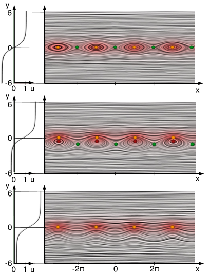
Figure 1: Stuart vortices in various convecting frames. The mean velocity profile is shown at the left. The Stuart vortices are depicted by visualizing the instantaneous velocity field using line integral convolution. The coloring is determined by vorticity; more intense red corresponds to higher vorticity. The critical points of standard velocity field topology are displayed as red (centers) and green (saddles) spheres. The maxima of the vorticity are added as orange spheres.

The Stuart vortices are depicted in Fig. 1 as streamlines using planar line integral convolution (LIC) Cabral:1993 ; Stalling:1995 . The top picture represents Eqs. (1) and shows the famous cat eyes in a periodic sequence of centers (vortices) and saddles for a vortex-fixed frame of reference ($u_{c}=0$). The middle picture depicts the same structures but in a frame of reference moving to the left with the lower stream at velocity $(-0.7,0)$, or, equivalently, the vortices moving to the right at $u_{c}=0.7$. The centers and saddles are displaced towards the slower stream. The bottom picture illustrates the same flow with a frame of reference moving at velocity $(-1.2,0)$, i.e. $u_{c}=1.2$ in Eq. (1). Now, no zeros are observed. These pictures recall the well-known fact, emphasized in many textbooks in fluid mechanics, that velocity field topology strongly depends on the frame of reference, i.e. is not Galilean-invariant. In case of the Stuart solution, one might argue that the frame of reference convecting with the structures is the most natural one. However, the convection velocity of a jet and many other flows depend on the streamwise position, i.e., generally no single natural frame of reference exists for topological considerations.

The saddles and centers of a Stuart solution are not only zeros of the velocity field but also zeros of the material acceleration field

$$\mathbf{a}=D_{t}\mathbf{u}=\partial_{t}\mathbf{u}+\mathbf{u}\cdot\nabla\mathbf{u}.$$ (2)

Here, $\partial_{t}$ represents the partial derivative with respect to time, $\nabla$ the nabla operator and the dot $\cdot$ the tensor contraction. The acceleration zeros are derived from a Galilean-invariant field and do not depend on the chosen inertial frame of reference. Figure 2 illustrates the acceleration field as height field.

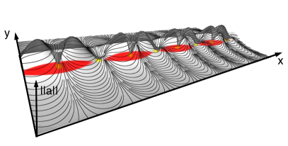
Figure 2: The acceleration field of convecting Stuart vortices. The coloring at the bottom is determined by the vorticity. The height field shows the acceleration magnitude and the curves depict integral lines of the acceleration vector field. The yellow spheres highlight the acceleration minima, orange spheres vorticity maxima. Note that center-like acceleration minima and vorticity maxima coincide (orange spheres hide yellow spheres).

The zeros of the acceleration field and the local minima of the acceleration magnitude (yellow spheres) coincide in this example. In general, the latter quantity is a superset of the first. The acceleration minima, however, enable to identify vortices and saddles in case of a non-uniform convection velocity.

II.2 Oseen vortex pair

In this section, a pair of equal Oseen vortices in ambient flow is considered. They rotate around the origin at constant distance $R=1/\sqrt{2}$ with uniform angular velocity $\Omega$. Let $\mathbf{x}_{i}=(x_{i},y_{i})$, $i=1,2$ be the centers of the two vortices. Then,

$$x_{1}= \!R\>\cos\Omega t,\quad y_{1}=R\>\sin\Omega t,$$ (3a)

$$x_{2}= \!-R\>\cos\Omega t,\quad y_{2}=-R\>\sin\Omega t.$$ (3b)

The induced velocity $u_{\theta}$ of a single Oseen vortex in the circumferential direction $\theta$ is given by

$$u_{\theta}(r)=\frac{\Gamma}{2\pi\>r}\>\left(1-e^{-\left(r/r_{c}\right)^{2}}\right),$$ (4)

where $r$ is the distance from the center of the vortex, $r_{c}$ determines the core radius and $\Gamma$ is the circulation of the vortex.

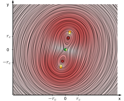
Figure 3: Depiction of two co-rotating Oseen vortices by their instantaneous streamlines using line integral convolution. The color-coding is determined by the acceleration magnitude; more intense red encodes higher values. The minima of the acceleration magnitude are marked by yellow spheres. For comparison, the critical points of standard velocity field topology (green and red spheres) and the maxima of the vorticity (orange spheres) are added.

In our example, $r_{c}$ is chosen as $0.5$ and $\Gamma$ as $2\pi$. The velocity of each vortex, cf. Eq. (3), corresponds to the induced velocity, cf. Eq. (4), i.e. $R\Omega=u_{\theta}(2R)$. The diffusion of vorticity is ignored to keep this analytical example simple. Figure 3 illustrates the Oseen vortex pair as described by Eq. (3) and Eq. (4). Here, the instantaneous streamlines can be inferred from the planar LIC.

Red and green spheres mark the corresponding critical points of the velocity field. Regions of large acceleration are marked by red. The minima (zeros) of the acceleration field are denoted by yellow circles. It should be noted that the maxima of the vorticity (indicated by orange spheres) are much closer to the minima (zeros) of the acceleration than to the zeros of the velocities. This difference is insignificant for ’frozen’ vortices but increases with increasing angular rotation. Hence, the difference is correlated with the radial acceleration of the vortex motion. Only a non-inertial co-rotating frame of reference minimizes the difference between vorticity maximum and the center of the velocity field.

It may be noted that any definition of feature points is based on the concept of an ’idealized template’, like a slowly accelerating saddle or vortex — as compared to the surrounding acceleration maximum. And any definition can be challenged by constructed limiting examples. In the example of an Oseen vortex pair, the limit of infinitely fast rotation of the vortices around their center constitutes such an example. However, this kinematic example would violate the Biot-Savart law, i.e. is not physically realizable.

II.3 Simple 3D flow

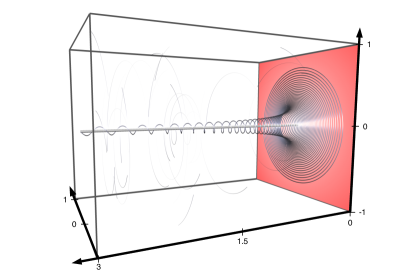
Figure 4: Depiction of a simple three-dimensional stationary flow field. The particle trajectories are indicated by the illuminated streamlines. In the center, the vortex core line is extracted as minimal line of the acceleration magnitude. Note that the particles along the vortex core line have non-zero acceleration.

Following Wu et al. Wu2005axial , we consider a simple linear velocity field with swirl and strain. The velocity field is given by

$$u = -0.75x-100y,$$

$$v = -0.75y+100x,$$ (5)

$$w = 1.5z.$$

The material acceleration $\mathbf{a}=(a_{u},a_{v},a_{w})$ of this field is given by

$$a_{u} = -9999.4375x+150y,$$

$$a_{v} = -9999.4375y-150x,$$ (6)

$$a_{w} = 2.25z.$$

In Fig. 4, some streamlines of this field are randomly placed in the volume. One streamline is emphasized showing swirling motion around the vortex core line (z-axis). The points on the core line are minima of the acceleration magnitude of the flow field with respect to a two-dimensional cross-section. Using the terminology of three-dimensional scalar field topology, such lines are called valley lines or minimal lines. They can be extracted from the acceleration magnitude field without prior knowledge of the corresponding cross-sections. In this example, the values of the acceleration are non-zero everywhere along the line. While for two-dimensional fields, the centripetal acceleration of a vortex always induces a zero point, this characterization is not transferable to the three-dimensional case. Now, minimal lines provide a meaningful generalization of the two-dimensional feature points to the three-dimensional setting.

III Feature Extraction

Our feature extraction pipeline consists of three steps: (1) spatial feature extraction, resulting in isolated feature points; (2) computation of the temporal evolution of these points; and (3) spatiotemporal filtering of the resulting structures, cf. Fig.5.

First (Sec. III.1), distinguished feature points are defined. One important implication of this definition for the pressure field is described in Sec. III.2. Finally, we describe a mathematical model for the extraction and tracking algorithm (Sec. III.3).

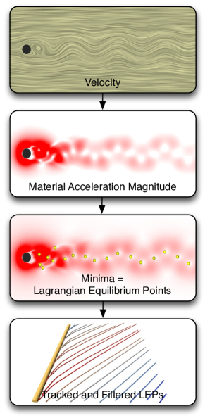
Figure 5: Pipeline of the proposed approach: After computing the acceleration magnitude field from the velocity, its minima are extracted, which are referred to as Lagrangian Equilibrium Points (LEPs). These LEPs are tracked over time and prioritized by a spatiotemporal importance measure. The importance measure combines a spatial strength and the lifetime of the feature.

III.1 Acceleration feature points

In this section, the definition of the considered feature is introduced. Starting point is a critical review of the velocity snapshot topology. Topological analysis of velocity fields has been successfully applied for examination of flow fields with a distinguished frame of reference. However, its applicability is limited, as location and number of critical points depend on the frame of reference. The goal of the current study is a definition of an alternative feature concept, which generalizes the snapshot topology in a local sense and overcomes the above-mentioned limitations. The feature point definition is motivated by the observations in the previous examples and the following three requirements:

(R1) Correspondence to velocity topology: A flow field is called steady, if there exists a distinguished frame of reference for which the vector field is stationary, i.e., it does not change in time. Such flow fields consist of frozen convective structures. They satisfy Taylor’s hypothesis taylor1938spectrum . With respect to this distinguished frame of reference, critical points of the velocity field correspond to the position of vortex cores and saddles. This concept is not applicable to unsteady flow fields, since there is no such distinguished frame of reference. Aiming for a generalization of velocity topology, the newly defined feature points should coincide for steady flow fields with the zeros of the velocity field. This also means that the classification of the points as saddles or centers is preserved. Note that this requirement is not fulfilled by Haller’s definition of an objective vortex Haller2005jfm . Rotational invariant features cannot distinguish saddles and centers.

(R2) Galilean invariance: A Galilean-invariant feature identifier reveals the same structures when changing the frame of reference.

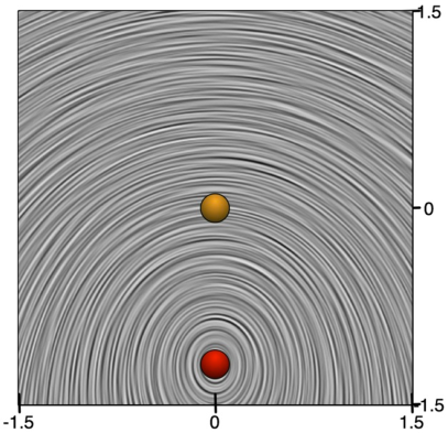
(a) Convecting center

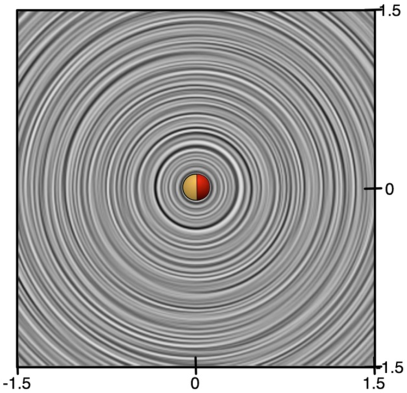
(b) Distinguished frame of reference

Figure 6: Convecting Oseen vortex displayed with respect to two different reference frames. A dense streamline visualization builds the background texture for both images. The maxima of the vorticity are marked by orange spheres. They coincide with the acceleration minima which are therefore not shown in both images. The fixed-points of the velocity field are represented as a red sphere. The vorticity maximum reveals a vortex core moving along the x-axis. In image (a), this point does not coincide with the center of the streamlines. Applying a Galilean transformation such that the resulting flow is steady leads to a convected frame of reference (b) revealing a different picture. Now the fixed point coincides with the maximum of vorticity and the minimum of the acceleration.

An example illustrating the influence of a Galilean transformation on the velocity field and its feature points is illustrated in Fig. 6. Let $\mathbf{v}(\mathbf{x},t)$ be a time-dependent vector field with a single Oseen vortex, Eq. 4 with $r_{c}=2$, $\Gamma=8\pi$, convecting with constant velocity $\left(x_{0}(t)=v_{0}t,y_{0}(t)=0\right)$ from left to right. The instantaneous velocity field for one point in time is shown in Fig. 6 (a) including the maximum of the vorticity (orange) and the fixed point (red). The two points do not coincide. Since this is a steady flow field, there exists a distinguished frame of reference moving with the center, that can be reached by a Galilean transformation. The resulting velocity field is shown in Fig. 6 (b). While the flow behavior itself is not changed by the transformation, the visual output is different. In particular, both feature points now coincide.

(R3) Lagrangian viewpoint: To guarantee a physically sensible feature identifier, we focus on particle motion. This Lagrangian viewpoint implies the focus on Galilean-invariant properties of fluid particles, but it does not include tracking finite-time fluid particle motion. This restricted Lagrangian viewpoint is consistent with the general notion of ’Lagrangian coherent structures.’

These requirements and the observations from Sec. II suggest to relate feature points to the material acceleration field. The particle acceleration $\mathbf{a}$ is the total derivative of the flow field ${\bf u}$. In other words, the acceleration in a space-time point $({\mathbf{x}},t)$ is given by Eq. (2).

Definition: A minimum of the magnitude of the material acceleration $\|{\mathbf{a}}\|$ is called acceleration feature point. Such points can be classified on the basis of the Jacobian of the velocity field, $\nabla\mathbf{u}$. A feature point is called saddle-like if its eigenvalues are real and center-like if its eigenvalues are complex. A feature trajectory is defined by the temporal evolution of a minimum in the acceleration field.

In the following, this definition is shown to satisfy requirements R1 to R3. Let $\mathbf{x}_{0}$ be a zero of the velocity field $\mathbf{u}(\mathbf{x}_{0},t)\equiv 0$. This implies that the material acceleration $\mathbf{a}|_{\mathbf{x}_{0}}=\left(\partial_{t}\mathbf{u}+\mathbf{u}\cdot\nabla\mathbf{u}\right)|_{\mathbf{x}_{0}}=0$ vanishes at $\mathbf{x}_{0}$. Thus, the minima of the acceleration magnitude are a superset of acceleration zeros and these zeros are a superset of the critical points of the velocity field. Hence, acceleration feature points can be considered to be a generalization of the critical points of the velocity fields. Acceleration is a Galilean-invariant quantity. It is computed from the velocity using the material or Lagrangian derivative that links the Eulerian to the Lagrangian viewpoint Panton1984book . Moreover, acceleration feature points satisfy all requirements R1 to R3.

The acceleration feature points can exhibit vortex- as well as saddle-like behavior, depending on the eigenvalues of the velocity Jacobian. Real eigenvalues correspond to saddles while a complex-conjugate eigenvalue pair indicates a vortex. Alternative synonymous discriminants have been proposed for 2D flows: Goto & Vassilicos Goto2006pf show that saddles are associated with sources of the material acceleration field while vortices correspond to sinks. One advantage of their definition is that it relies purely on the acceleration without reference to the velocity Jacobian. Basdevant & Philipovitch Basdevan1994pd critically assess the use of the Weiss criterion as discriminant.

III.2 Implications of acceleration feature points

Another perspective onto the acceleration minima is given by their relation to the pressure gradient via the incompressible Navier-Stokes equation:

$${\mathbf{a}}({\mathbf{x}},t) =-\frac{1}{\rho}\>\nabla p({\mathbf{x}},t)+\nu\,\Delta{\mathbf{u}}({\mathbf{x}},t),$$ (7)

$$0 =\hskip 7.0pt\nabla\cdot{\mathbf{u}}({\mathbf{x}},t)\text{,}$$

where $p$ is the pressure of the flow field, $\rho$ and $\nu$ are the kinematic viscosity and density of the fluid, respectively, and $\Delta$ is the spatial Laplacian operator. For ideal flows, the equations reduce to the Euler equation:

$${\mathbf{a}}({\mathbf{x}},t) =-\frac{1}{\rho}\>\nabla p({\mathbf{x}},t),$$ (8)

$$0 =\hskip 7.0pt\nabla\cdot{\mathbf{u}}({\mathbf{x}},t)\text{.}$$

Then, local extrema of the pressure field, which are zero points of the pressure gradient coincide with zeros of the acceleration field. In this case, the above defined acceleration feature points form a superset of local extrema of the pressure field, the minima of which are often associated with vortices.

III.3 Feature Point Extraction Strategy

A second task, besides the definition of physically appropriate feature points, is the selection of a mathematical model that serves as basis for an algorithmic implementation. The selection of a mathematical framework is guided by the following criteria:

(C1) It should facilitate a robust and efficient extraction without subjective parameters to enable an unsupervised extraction of the structures.

(C2) It should allow to generate a feature hierarchy based on an intrinsic filtering mechanism. This eases the interpretation of the results and becomes necessary as soon as one moves on from simple showcases or when the data exhibit high feature densities.

(C3) It should allow for tracking of features over time, based on neighborhood relations.

From a mathematical point of view, extrema and ridges of scalar fields can be subsumed under the framework of scalar field topology. This provides access to many powerful algorithmic tools developed for extraction and tracking of topological structures in scalar fields. The algorithm to extract minima of scalar fields used in this paper is based on discrete Morse theory Forman1998b . It is purely combinatorial and guarantees topological consistency of the extracted structures Reininghaus2010a . The robustness of the algorithm and lack of any algorithmic parameter allow an unsupervised extraction of structures. This guarantees the applicability of the methods to large data sets. In the following, we will briefly describe the used methods and summarize the concept of discrete Morse theory.

Combinatorial extraction of two-dimensional scalar field topology – Typically, scalar field topology is extracted by analyzing the gradient of the scalar function. This approach utilizes derivatives that amplify noise when computed in a discrete setting. In contrast, combinatorial methods do not rely on interpolation or derivatives. Therefore, we decided to use a combinatorial setting, here, following the ideas of Reininghaus et al. Reininghaus2010a . Note that our data is given on a polygonal grid for each time slice.

In the following, we briefly describe how to extract scalar field topology using the aforementioned approach: The grid that holds the data is transferred to a polygonal graph. In this graph, each node represents a $d$-dimensional face (point, edge, polygon) and each link represents the connection between two adjacent faces. In accordance to Forman Forman1998b , the combinatorial gradient field is given as a matching on this graph. The critical points are represented by the unmatched nodes and the streamlines are alternating paths with respect to the matching. An optimization algorithm enforces the matching to represent the actual analytic gradient field best. Loosely speaking, it has to be assured that a combinatorial stream line corresponds best to the analytical stream lines. A couple of algorithmic implementations of this idea have been proposed; we follow the approach presented by Robins et al. robins10 .

Generating a feature hierarchy for acceleration feature points – One way to approach the problem of a high feature density are statistical methods. Another way, pursued in this work, is to facilitate an importance measure to build a feature hierarchy. A commonly used importance measure for critical points in context of scalar field topology is persistent homology Edelsbrunner2008 .

Persistence measures the stability of critical points with respect to changes in the data as introduced by noise, for instance. To do so, persistence analyzes the topological changes of the sublevel sets of a scalar function. At critical points, the topology of the sublevel sets changes by increasing the sublevel parameter. In two dimensions, there are four events possible: First, a new connected component in the sub-level set can be born. This happens at a minimum. Furthermore, two connected components can merge, which occurs when the parameter $t$ passes the value of a saddle. Third, a new hole can also be born at a saddle. Last, a hole in a connected component can die. This occurs at a maximum.

The persistence value of the critical points is determined in the following way: A new-born connected component is labeled with the associated minimum. At a saddle, two connected components merge that are labeled with two different minima. The persistence value for the saddle and the minimum with the higher scalar value is defined as their scalar value difference. The merged component is labeled with the remaining minimum. A maximum is paired with the saddle with the highest function value and, again, their persistence value is defined as their scalar value difference.

Algorithmically, persistence can be computed in two dimensions by an approach that can also be used to compute the matching, see Ref. Reininghaus2010a . For two-dimensional fields of reasonable resolution, the implementation computes persistence in a few seconds. This enables us to analyze time-dependent fields with many time slices. The advantage of this algorithm is that it not only computes the persistence values for the critical points but it is also able to simplify the combinatorial gradient field following the hierarchy introduced by persistence. This can be used to reduce noise and therefore facilitates the tracking of the critical points in the next step.

Note that critical points that are paired by persistence are not necessarily adjacent. For a simple example illustrating the concept of persistent homology, we refer the reader to Figure 7.

Temporal feature development – To get an understanding of the temporal evolution of acceleration feature points, the minima are tracked over time. In the context of discrete Morse theory, one can make use of combinatorial feature flow fields (CFFF), as proposed in Ref. Reininghaus2011 . The basic idea of this tracking algorithm is to construct a discrete gradient field in space-time, describing the development of the acceleration minima, such that tracking of those minima results in an integration of the discrete gradient field. The approach constructs two fields: A forward and a backward field representing the destination of a critical point in forward or backward direction, respectively. Two minima of two adjacent time slices are uniquely connected to each other, if they are connected in the forward as well as in the backward field. Intuitively, these two minima are uniquely connected if they fall into each other’s basin, see Figure 7. The result of this tracking is a set of temporal feature lines without mergers and splits. By further incorporating the aforementioned spatiotemporal gradient fields, we were able to extract the mergers that occur for vortex core lines in a two-dimensional setting. To do so, we utilize the forward tracking field to connect the end of a uniquely tracked minima line to another minima line in space time. The general approach is described in Kasten2012b .

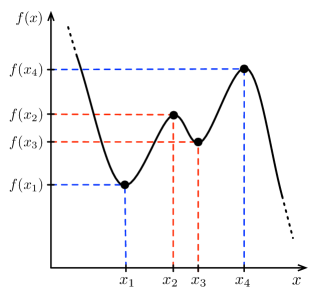
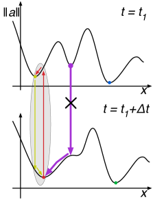
Figure 7: (a): The employed spatial feature importance is given by the persistent homology of the critical points. It measures how strong a minimum is, compared to its neighbors. This is achieved by correctly pairing critical points and quantifying their height difference. The image shows such a pairing, e.g., the critical points at $x_{2}$ and $x_{3}$. (b): To extract the evolution of the acceleration feature points in time, the minima are tracked. The applied method utilizes the concept of combinatorial feature flow fields (CFFF). In this setting, two minima of adjacent time slices are uniquely connected, if they lie in the basin of each other.

Generating a feature hierarchy for temporal feature lines – A typical importance measure applied for time dependent features is the concept of feature lifetime. While leading to much simpler results, such filter methods are purely based on temporal measures. They ignore pronounced short-lived features, which can play a significant role for the flow. Therefore, the temporal importance measure, given by the feature lifetime, should be combined with a spatial feature strength. The CFFF approach allows for a straightforward incorporation of persistent homology as spatial importance measure for feature lines. In this paper, the spatiotemporal importance measure is defined by integrating persistence along the feature line, e.g., by accumulating all persistence values along the line. Since the measure is not normalized, the lifetime of the feature is inherently depicted by this measure – longer living features are more important if all structures have the same spatial strength. Using this importance measure, it is possible to filter out short-living weak features.

IV Results for free shear flows

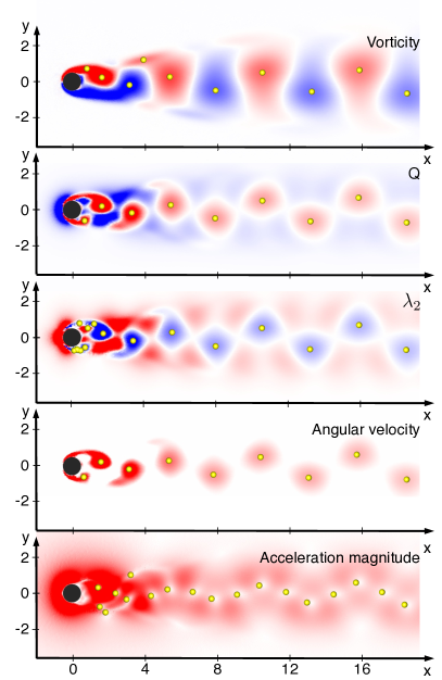
Figure 8: Visualization of a cylinder wake snapshot. Five vorticity-related quantities are depicted by color maps (red: positive values, blue: negative, gray: zero): (1) vorticity; (2) Okubo-Weiss parameter; (3) $\lambda_{2}$; (4) absolute value of the imaginary part of the eigenvalues of the velocity Jacobian – corresponds to the angular velocity; (5) material acceleration magnitude. The yellow spheres depict the extremal points typically used as features for the respective quantity.

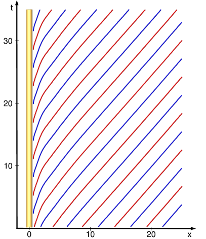
Figure 9: Tracked vortices of the cylinder wake in an $x$-$t$-view. Red (blue) marks positive (negative) rotation the vortices.

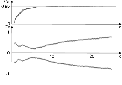
Figure 10: Plots of the streamwise velocity component $u_{v}$ (top) and the transverse displacement $y_{v}$ (bottom) along tracked vortices. Note that each figure contains the history of many vortex evolutions from roll-up to convection out of the domain. Hence, several lines can be seen in each curve.

Three free shear flows are investigated: the cylinder wake (Sec. IV.1), the mixing layer (Sec. IV.2), and the planar jet (Sec. IV.3). These configurations represent different levels of spatiotemporal complexity from the periodic wake to the broadband dynamics and vortex pairing of the mixing layer and jet. The first two flows share a pronounced uniform far-wake convection velocity, while the jet structures move slower with streamwise distance.

Focus is placed on the vortex skeleton as identified by the acceleration feature points. Pars pro toto, we perform a statistical analysis for the wake (Sec. IV.1), investigate the vortex merging of the mixing layer (Sec. IV.2), and employ the persistence-filter of LEPs for the jet (Sec. IV.3).

All flows are described in a Cartesian coordinate system $\mathbf{x}=(x,y)$, of which the abscissa $x$ points in streamwise direction and $y$ in transversal direction. The origin is located in the source of the shear flow, i.e. center of the cylinder for the wake, center of the inflow for the mixing layer and center of the orifice for the jet. The velocity $\mathbf{u}=(u,v)$ is expressed in the same system, $u$ and $v$ being the $x$- and $y$-components of the velocity. The time is denoted by $t$, the pressure by $p$ and the material acceleration by $\mathbf{a}$. All quantities are non-dimensionalized with a characteristic length-scale $L$, a characteristic velocity $U$ and the density of the fluid $\rho$. $L$ denotes the cylinder diameter for the wake, the vorticity thickness for the mixing layer, and the width of the origin for the planar jet. $U$ corresponds to the oncoming flow for the wake, to the velocity of the upper (faster) stream for the mixing layer, and to the maximum velocity at the orifice for the jet.

IV.1 Cylinder wake

Starting point is a benchmark problem of the data visualization community: periodic vortex shedding behind a circular cylinder. The Reynolds number is set to $100$, which is well above the critical value for vortex shedding at $47$ Zebib1987jem ; Jackson1987jfm and well below the critical value for transition-related instabilities around $180$ Zhang1995pf ; Williamson1996arfm . The flow is simulated with a finite-element method solver with third-order accuracy in space and time, like in Noack2003jfm . The rectangular computational domain $(x,y)\in[-10,30]\times[-15,15]$ without the disk $K_{1/2}(0)$ for the cylinder is discretized by 277,576 triangular elements. The numerical time step for implicit time integration is $0.1$, which also corresponds to the sampling frequency for the snapshots.

Figure 8 shows five vorticity related quantities of a cylinder wake snapshot. The vorticity field depicts the separating shear-layers rolling up in a staggered array of alternating vortices. The yellow balls mark the extrema, revealing the known fact that the ratio between the transverse of vortex displacement and the wavelength slightly increases downstream with vortex diffusion. The second subfigure shows the Okubo-Weiss parameter $Q=\|\mathbf{S}^{-}\|^{2}-\|\mathbf{S}^{+}\|^{2}$ marking the maxima with balls. This parameter employs the velocity Jacobian $\nabla\mathbf{u}$ and compares the norm of the symmetric shear tensor $\mathbf{S}^{+}\!=\!\frac{1}{2}\left[\nabla\mathbf{u}+\left(\nabla\mathbf{u}\right)^{t}\right]$ and with the norm of the antisymmetric one $\mathbf{S}^{-}\!=\!\frac{1}{2}\left[\nabla\mathbf{u}-\left(\nabla\mathbf{u}\right)^{t}\right]$. In the center of a radially symmetric vortex, $Q=\|\mathbf{\omega}\|^{2}>0$, since $\|\mathbf{S}^{+}\|$ vanishes and $\|\mathbf{S}^{-}\|$ becomes the norm of the vorticity $\|\mathbf{\omega}\|$. At a saddle point $Q=-\|\mathbf{S}^{+}\|^{2}<0$. Hence, maxima of $Q$ can be associated with vortex centers and minima with saddles. The third subfigure shows $\lambda_{2}$. Its extrema are marked by balls and indicate vortex centers. $Q$ and $\lambda_{2}$ are generally considered to provide synonymous information. The absolute value of the imaginary part of the Jacobian $\nabla\mathbf{u}$ is shown in the fourth subfigure. This quantity characterizes the angular frequency of revolution of a neighboring particles. Hence, its maxima marked by yellow balls indicate vortex centers. Finally, the magnitude of the material acceleration field is depicted. The minima (zeros) mark both vortex centers and saddles, i.e. twice as many points in the vortex street. These two features are distinguished based on the velocity Jacobian: two positive eigenvalues of the velocity Jacobian are associated with a saddle, a complex conjugate pair with a vortex.

In the vortex street, all five vortex criteria provide nearly identical locations. In the boundary-layer and in the near-wake of the cylinder there are pronounced differences. Mathematically, the vortex criteria rely on quite different formulae. They cannot be expected to exactly coincide except for pronounced flow features, e.g. axis-symmetric vortices. In addition, the cylinder boundary introduces a singular line $\mathbf{u}=\mathbf{0}$, thus amplifying the differences between the vortex criteria.

Figure 9 shows the spatial-temporal vortex evolution, based on the tracked acceleration feature points. In the far-wake, a uniformly convecting von Kármán vortex street is observed. In the near-wake, the convection speed is significantly slower. This aspect is highlighted in Fig. 10 (first subfigure). The streamwise velocity of each vortex $u_{v}$ is a monotonically increasing function from 0.03 to about 0.85. The asymptote corresponds to the literature value Williamson1996arfm .

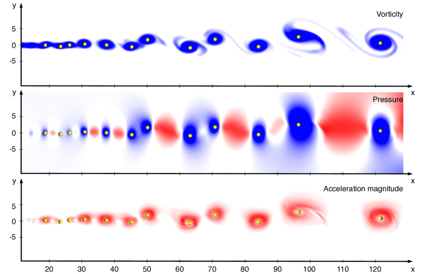
Figure 11: Visualization of a mixing layer snapshot. Comparison of vorticity (top), pressure (middle) and acceleration (bottom). The color scheme is blue (red) for negative (positive) values. The yellow spheres represent pronounced vortex acceleration feature points.

The transverse spreading of the vortex street, noted in Fig. 8, is quantified in the following subfigure with the transverse location $y_{v}$.

It should be noted that tracked acceleration feature points can be seen as markers of coherent structures. The acceleration-based framework provides a convenient means for determining convection velocities and evolution of spatial extensions. The following investigations of the mixing layer and the jet flow emphasize this aspect.

IV.2 Mixing layer

The second investigated shear flow is a mixing-layer with a velocity ratio between upper and lower stream of 3:1, following earlier investigations of the authors Comte1998ejmb ; Noack2004swing ; Noack2005jfm . The inflow is described by a $\tanh$ profile with a stochastic perturbation. And the Reynolds number based on maximum velocity and vorticity thickness is 500. The flow is computed with a compact finite-difference scheme of 6th order accuracy in space and 3rd oder accuracy in time. The computational domain $(x,y)\in[0,140]\times[-28,28]$ is discretized on a $960\times 384$ grid. The sampling time for the employed snapshots is $\Delta t=0.05$ corresponding 1/10 of the computational time step.

In contrast to the space- and time-periodic Stuart solution, the mixing layer generally shows several vortex pairing events. In Fig. 11, the distance between vortex acceleration feature points (marked by balls) are seen to increase in streamwise direction as result of vortex merging. Furthermore, the locations of the acceleration feature points nicely correlate with the local maxima of the vorticity (top), the local minima of the pressure (middle) and the local minima of the magnitude of the material acceleration (bottom). The correlation between vorticity maxima and pressure minima in free shear flows is well documented in the literature. The correlation between pressure and acceleration magnitude minima may be inferred from the non-dimensionalized Euler equation $\mathbf{a}=-\nabla p$, governing the predominantly inviscid dynamics of the mixing layer (see Sec. III). A pressure minimum (or maximum) implies $\nabla p=0$ and thus $\mathbf{a}=0$.

The vortex merging events are shown in Fig. 12.

Figure 12: Spatiotemporal evolution of vortices in the mixing-layer. The top part of the figure shows the acceleration magnitude field and LEPs at the final time considered. The bottom figure marks the tracked acceleration feature points over approximately 5 downwash times. Numerous vortex merging events can be identified. The size and coloring of the vortex skeleton is determined by vorticity – more intense blue corresponds to lower vorticity. Note that the vorticity is negative everywhere.

Upstream, many Kelvin-Helmholtz vortices are formed. In streamwise direction numerous merging events can be identified, approximately 2 successive vortex mergers in the domain shown. Not all crossing of $x,t$-curves mark mergers since vortex pairs may rotate around their center before eventual merging. The figure strongly suggests a nearly constant streamwise convection velocity, as expected from literature results and contrary to the cylinder wake dynamics.

IV.3 Planar jet

Finally, the spatiotemporal evolution of the planar jet is investigated. Like the mixing layer, the jet shows a number of vortex mergers leading to a reduction of the characteristic frequency. As additional complexity, the convection velocity is not constant but decreases in streamwise direction.

All quantities are normalized with the jet width $D_{j}$ and maximum jet velocity $U_{j}$. The flow is a weakly compressible isothermal 2D jet with a Mach number of $M\!a_{j}=0.1$ and a Reynolds number of $Re_{j}=D_{j}U_{j}/\nu_{\infty}=500$. The inflow velocity profile is given by a hyperbolic tangent profile like in Freund2001jfm :

$$u(r)=U_{\infty}+\frac{(U_{j}-U_{\infty})}{2}\left[1-\tanh\left[b\left(\frac{r}{r_{0}}-\frac{r_{0}}{r}\right)\right]\right].$$

Here, a uniform 1% co-flow $U_{\infty}=0.01U_{j}$ is added to avoid vortices with arbitrarily long residence time in the computational domain. The slope of the $\tanh$ profile is characterized by $b={r_{o}}/{4\delta_{\theta}}$ and the momentum thickness of the shear layer is $\delta_{\theta}=0.05r_{o}$. The initial mean temperature was calculated with the Crocco-Busemann relation, and the mean initial pressure was constant.

The natural transition to unsteadiness is promoted by adding disturbances in a region in the early jet development near the inflow boundary $x_{o}=-0.5$ :

$$v(x,y)=v(x,y)+\alpha U_{c}e^{-\frac{(x-x_{o})^{2}}{\lambda_{x}^{2}}}(f_{1}(y)+f_{2}(y))$$ (9)

Here,

$$f_{1}(y)=\epsilon_{1}e^{-\frac{(y-y_{1})^{2}}{\lambda_{y}^{2}}},\qquad f_{2}(y)=\epsilon_{2}e^{-\frac{(y-y_{2})^{2}}{\lambda_{y}^{2}}},$$ (10)

where $U_{c}=0.5$, $\alpha=0.008$, $y_{1}=0.5$, $y_{2}=-0.5$, $\lambda_{x}=0.1$, $\lambda_{y}=0.1$ and $-1\leq\epsilon_{1},\epsilon_{2}\leq 1$ are random numbers.

The flow is defined in a rectangular domain $(x,y)\in[0,20]\times[-7,7]$. The adjacent sponge zone extends to $[-1.5,25]\times[-10,10]$. The whole domain is discretized on a non-uniform Cartesian with $2\,449$ points in $x$-direction and 598 points in $y$-direction. The compressible Navier-Stokes equation is solved by mean of a (2,4) conservative finite-difference scheme based on MacCormack’s predictor-corrector method Gottlieb1976mc with block-decomposition and MPI parallelization. The system may be closed by the thermodynamic relations for an ideal gas. Details of the equations, boundary conditions and solver can be inferred from Cavalieri2011jsv .

A stochastic inflow perturbation gives rise to small acoustic waves. These small acoustic perturbations provide an excellent test-case demonstrating the need and performance of persistence-based filtering. Figure 13 depicts a jet snapshot.

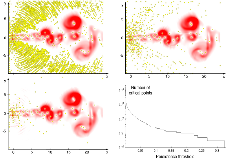
Figure 13: Persistence-based visualization of a jet snapshot. Top left to bottom left: Visualization of the snapshot for persistence threshold levels of $0\%$ (top left), $0.5\%$ (top right) and $2\%$ (bottom left) of the maximum. The color field depicts the acceleration magnitude – with a color map that ranges from white (zero) to red (positive). The yellow balls represent acceleration feature points filtered by their persistent homology with respect to the specified threshold levels.
Bottom right: Persistence distribution. The number of critical points after persistence-based filtering is plotted against the persistence threshold level.

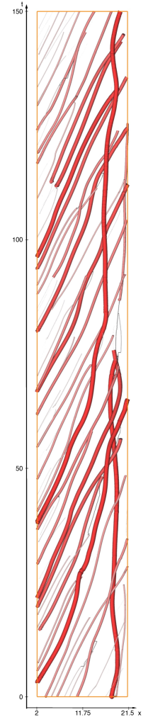
Figure 14: Spatiotemporal evolution of the vortex skeleton of the jet. The size and coloring of the vortex lines are determined by our spatiotemporal importance measure. The links between the individual vortices are shown as white gray lines.

Most of the acceleration feature points are associated low-amplitude sound waves from the random inlet perturbation (top figure). These acceleration feature points may be filtered out, ignoring those with low persistence (middle and bottom). The bottom figure shows only features associated with incompressible dynamics.

The spatiotemporal evolution of the vortex skeleton of the jet is visualized in Fig. 14 in a similar manner as the wake (Fig. 9) and the mixing-layer (Fig. 12). Clearly, vortex merging events and a streamwise decreasing convection velocity can be identified. In particular, some strong vortices remain for a long time near the exit. A three-dimensional close-up view is shown in Fig. 15.

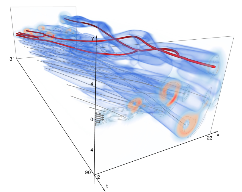
Figure 15: Close-up view of the vortex skeleton of the jet flow. The gray lines depict the extracted and filtered vortex cores. A few lines are visually highlighted by red coloring; they show a pronounced vortex merging event and the origin of the merged vortices. The acceleration is visualized by the blue volume rendering and the color coding in the front and back plane. For comparison, iso-lines of the vorticity are added to the front plane.

V Conclusion and outlook

We have proposed a novel feature extraction strategy for unsteady 2D flows. This strategy departs in important aspects from topology extraction of the instantaneous velocity field, starting from the velocity zeros. Instead of the velocity, the material acceleration field is analyzed, following Goto2006pf . Secondly, instead of acceleration zeros, the minima of the acceleration magnitude are identified. Thirdly, the acceleration feature points are tracked in time. Finally, a mathematically rigorous spatiotemporal hierarchy of the tracked minima is defined.

The acceleration feature points define topological elements of an unsteady flow with a number of discriminating features:

1. For steady flows, the acceleration feature points are a natural generalization of the critical points of vector field topology. Each critical point is an acceleration feature point. This implication may not hold generally in the other direction.

2. A critical point of a steady flow field remains an acceleration feature point in any inertial frame of reference. In other words, the acceleration feature points cannot vanish or be distorted by a uniform convection of a ’frozen’ flow field (Taylor hypothesis).

3. The acceleration feature points are independent of the inertial frame of reference, i.e. they are Galilean-invariant. This property is a trivial consequence of the material acceleration field as observable.

4. The concept of acceleration feature points is parameter-free. No integration windows, nor threshold criteria, etc. are needed. Note that the persistence level is not a free parameter, as it defines a feature hierarchy.

5. Acceleration is correlated with pressure by neglecting the viscous term. Suppose the pressure field has a minimum (in a vortex) or maximum (near a saddle point). Then, the pressure gradient vanishes and the Euler equation yields a vanishing material acceleration (implying trivially also a magnitude minimum).

6. The persistence measure introduces a rigorous hierarchy of acceleration feature points based on spatial characteristics, without the need of temporal filtering.

7. With the tracking of the acceleration feature points, the temporally integrated persistence emphasizes long-lived structures.

In short, identification of acceleration feature points naturally generalizes identification of critical points and exhibits new desirable or even necessary properties for a meaningful flow analysis.

Our framework follows Vassilicos’ group Goto2006pf in employing the Galilean-invariant material acceleration field as opposed to the velocity field. However, Vassilicos determines the zeros of this field, while our acceleration feature points are based on the more general notion of magnitude minima. This enables a robust, computationally inexpensive, derivative-free feature extraction — capable of coping with large noise levels in the data. Furthermore, using minima instead of zeros allows for a natural extension to three-dimensional flows. The concept of acceleration feature points follows Haller in the search of a Lagrangian Galilean invariant definition of saddles Haller2001physd and vortices Haller2005jfm , but provides a simple aggregate definition for both features. The hierarchy of the acceleration feature points can be determined from a single snapshot, i.e., no back-and-forward integration of fluid particles is required.

The framework has been applied to three free shear flows: periodic vortex shedding of a cylinder wake, a mixing layer with a small range of dominant frequencies, and a planar jet with broadband dynamics. In all cases, the acceleration feature points are cleanly distilled from the numerical data and they enable additional insights. For the wake flow, vortex-based statistics are possible, e.g., for determining the streamwise convection velocity. For the mixing layer, vortex merging events are specified in time and space. And for the jet, persistence is used to separate between aeroacoustic and hydrodynamic equilibrium points.

In the numerical analyses, only vortices have been considered. Here, vortices are acceleration feature points with imaginary eigenvalues of the velocity Jacobian. Analogously, saddles can be defined as acceleration feature points with real eigenvalues of this Jacobian matrix. Thus, the concept of acceleration feature points represents a unifying framework for the main generic features of 2D flows. Furthermore, it offers a computationally inexpensive alternative to the concept of the finite-time Lyapunov exponent Haller2001physd . We actively pursue a 3D generalization of the proposed feature extraction.

The Galilean-invariant generalization of critical points has no obvious analogues to connectors in topology. The very concept of connectors as boundary between different particles looses its meaning in a time-dependent flow field.

As outlook, 3D acceleration feature points (or lines and surfaces) with associated importance hierarchy and tracking technique may pave the path to future kinematic analyses of complex turbulent flows. A technique that extracts a hierarchy of the physically important points (and lines) of complex data will become invaluable as a first step in analysis. The required visualization methods are already correspondingly mature.

References

- [1] M. J. Lighthill. Attachment and Separation in Three Dimensional Flow. Oxford University Press, Oxford, 1st edition, 1963.
- [2] M. Tobak and D. J. Peake. Topology of three-dimensional separated flows. Ann. Rev. Fluid Mech., 14:61–85, 1982.
- [3] A. E. Perry and M. S. Chong. A description of eddying motions and flow patterns using critical-point concepts. Ann. Rev. Fluid Mech., 19:125–155, 1987.
- [4] D. Rodriguez and V. Theofilis. Structural changes of laminar separation bubbles induced by global linear instability. J. Fluid Mech., 655:280–305, 2010.
- [5] D. Rodriguez and V. Theofilis. On the birth of stall cells on airfoils. Theor. Comput. Fluid Dyn., 25:105–117, 2011.
- [6] L. Wang and N. Peters. The length-scale distribution function of the distance between extremal points in passive scalar turbulence. J. Fluid Mech., 554:457–475, 2006.
- [7] L. Wang and N. Peters. Length-scale distribution functions and conditional means for various fields in turbulence. J. Fluid Mech., 608:113–138, 2008.
- [8] S. Goto and J. C. Vassilicos. Self-similar clustering of inertial particles and zero-acceleration points in fully developed two-dimensional turbulence. Phys. Fluids, 18(11):115103–1..10, 2006.
- [9] H. Edelsbrunner and J. Harer. Persistent homology — a survey. In J. E. Goodman, J. Pach, and R. Pollack, editors, Surveys on Discrete and Computational Geometry: Twenty Years Later, volume 458, pages 257–282. AMS Bookstore, 2008.
- [10] J. Reininghaus, D. Günther, I. Hotz, S. Prohaska, and H.-C. Hege. TADD: A computational framework for data analysis using discrete Morse theory. In Proc. ICMS 2010, 2010.
- [11] J. Reininghaus, J. Kasten, T. Weinkauf, and I. Hotz. Efficient computation of combinatorial feature flow fields. IEEE Trans. Vis. Comput. Graph., to appear, 2012.
- [12] J.T. Stuart. On finite amplitude oscillations in laminar mixing layers. J. Fluid Mech., 29:417–440, 1967.
- [13] B. Cabral and L. C. Leedom. Imaging vector fields using line integral convolution. In Proceedings of the 20th Annual Conference on Computer Graphics and Interactive Techniques, SIGGRAPH ’93, pages 263–270, New York, NY, USA, 1993. ACM.
- [14] D. Stalling and H.-C. Hege. Fast and resolution independent line integral convolution. In Proceedings of the 22nd Annual Conference on Computer Graphics and Interactive Techniques, SIGGRAPH ’95, pages 249–256, New York, NY, USA, 1995. ACM.
- [15] J.Z. Wu, A.K. Xiong, and Y.T. Yang. Axial stretching and vortex definition. Phys. Fluids, 17:038108, 2005.
- [16] G. I. Taylor. The spectrum of turbulence. Proceedings of the Royal Society of London. Series A-Mathematical and Physical Sciences, 164(919):476–490, 1938.
- [17] G. Haller. An objective definition of a vortex. J. Fluid Mech., 525:1–26, 2005.
- [18] R.W. Panton. Incompressible Flow. John Wiley & Sons, New York, etc., 1984.
- [19] Claude Basdevant and Thierry Philipovitch. On the validity of the “Weiss criterion” in two-dimensional turbulence. Phys. D, 73(1-2):17–30, May 1994.
- [20] R. Forman. Morse theory for cell-complexes. Advances in Mathematics, 134(1):90–145, 1998.
- [21] V. Robins, P. Wood, and A. Sheppard. Theory and algorithms for constructing discrete Morse complexes from grayscale digital images. IEEE Transactions on Pattern Analysis and Machine Intelligence, 33(8):1646–1658, 2011.
- [22] J. Kasten, I. Hotz, B. R. Noack, and H.-C. Hege. Vortex merge graphs in two-dimensional unsteady flow fields. In Proceedings Joint EG - IEEE TVCG Symposium on Visualization, 2012.
- [23] A. Zebib. Stability of viscous flow past a circular cylinder. J. Engr. Math., 21:155–165, 1987.
- [24] C.P. Jackson. A finite-element study of the onset of vortex shedding in flow past variously shaped bodies. J. Fluid Mech., 182:23–45, 1987.
- [25] H.-Q. Zhang, U. Fey, B. R. Noack, M. König, and H. Eckelmann. On the transition of the cylinder wake. Phys. Fluids, 7(4):779–795, 1995.
- [26] C.H.K. Williamson. Vortex dynamics in the cylinder wake. Annu. Rev. Fluid Mech., 28:477–539, 1996.
- [27] B. R. Noack, K. Afanasiev, M. Morzyński, G. Tadmor, and F. Thiele. A hierarchy of low-dimensional models for the transient and post-transient cylinder wake. J. Fluid Mech., 497:335–363, 2003.
- [28] P. Comte, J.H. Silvestrini, and P. Bégou. Streamwise vortices in Large-Eddy Simulations of mixing layer. Eur. J. Mech. B, 17:615–637, 1998.
- [29] B. R. Noack, I. Pelivan, G. Tadmor, M. Morzyński, and P. Comte. Robust low-dimensional Galerkin models of natural and actuated flows. In W. Schröder & P. Tröltzsch, Fourth Aeroacoustics Workshop. Institut für Akustik und Sprachkommunikation, Technische Universität Dresden, 2004.
- [30] B. R. Noack, P. Papas, and P. A. Monkewitz. The need for a pressure-term representation in empirical Galerkin models of incompressible shear flows. J. Fluid Mech., 523:339–365, 2005.
- [31] J.B. Freund. Noise sources in a low Reynolds number turbulent jet at Mach 0.9. J. Fluid Mech., 438:277–305, 2001.
- [32] D. Gottlieb and E. Turkel. Dissipative two-four method for time dependent problems. Math. of Comp., 30(136):703–723, 1976.
- [33] A. V. G. Cavalieri, G. Daviller, P. Comte, P. Jordan, G. Tadmor, and Y. Gervais. Using large eddy simulation to explore sound-source mechanisms in jets. J. Sound Vibr., 330(17):4098–4113, 2011.
- [34] G. Haller. Distinguished material surfaces and coherent structures in 3D fluid flows. Phys. D, 149(4):248–277, 2001.