Self Organizing strategies for enhanced ICIC (eICIC)

Abstract

Small cells have been identified as an effective solution for coping with the important traffic increase that is expected in the coming years. But this solution is accompanied by additional interference that needs to be mitigated. The enhanced Inter Cell Interference Coordination (eICIC) feature has been introduced to address the interference problem. eICIC involves two parameters which need to be optimized, namely the Cell Range Extension (CRE) of the small cells and the ABS ratio (ABSr) which defines a mute ratio for the macro cell to reduce the interference it produces. In this paper we propose self-optimizing algorithms for the eICIC. The CRE is adjusted by means of load balancing algorithm. The ABSr parameter is optimized by maximizing a proportional fair utility of user throughputs. The convergence of the algorithms is proven using stochastic approximation theorems. Numerical simulations illustrate the important performance gain brought about by the different algorithms.

I Introduction

Small cells have been identified as one of the most promising solutions for coping with the expected traffic growth in the coming years. The low transmit power of these nodes makes their footprint very small, limiting the amount of macrocell traffic they can offload. To enhance the offloading capabilities of small cells, the CRE (CRE) mechanism has been introduced in the 3GPP standard allowing a small cell to extend its coverage by increasing the CIO (CIO) parameter. The CIO defines the attachment rule of UE to the small cell. The macro BS which previously served the UE at the small cells’ extended coverage zone may now strongly interfere them. An interference mitigation mechanism has been proposed to protect these UE by muting almost all macro BS transmissions on a certain portion of subframes, thus letting small cells serve their users with less interference. The muted sub frames are denoted as ABS (ABS). The combination of these two mechanisms has been described in 3GPP [1, Section 16.1.5] under the name of eICIC (eICIC).

Two different parameters are involved in eICIC: the CIO which in our scenario is applied only to the small BS to offload macro BSs, and the ABSr (ABSr), namely the percentage of the muted subframes at the macro BSs. Although the principle of eICIC has been described in 3GPP, its actual implementation is not clearly specified, and in particular, the way to set these eICIC parameters which may be critical for the cell performance.

Previous contributions on eICIC focus on performance gain brought about by this feature in a static heterogeneous network [2, 3, 4]. In [5] and [6], the eICIC parameters are optimized for a static scenario. The ABSr optimization problem has been treated for a dynamic environment in [7] assuming fixed CIO. The problem of optimizing both CIO and ABSr has been studied in [8, 9] using a centralized approach. The solution is computationally demanding and can be implemented as a management plane solution.

The purpose of this paper is to propose efficient and distributed SON (SON) algorithms for optimizing both the CIO and the ABSr parameters using stochastic approximation techniques [10, 11]. We use a distributed load balancing objective for the small cell CIO optimization [12]. Then we propose a distributed solution for optimizing the ABSr at the small BS which in turn request these ABSr from their interfering macro BS. ABSr optimization algorithms are proposed using objective functions based on a PF (PF) utility of users’ throughputs. Different strategies for scheduling small BS’ users during the muted subframes of the macro BS are studied.

The contributions of the paper are the following:

• A load balancing SON algorithm for CRE optimization using results from [12].

• A distributed scheme for optimizing the ABSr of the macro BS.

• Two SON algorithms based on SA (SA) for optimizing ABSr using PF utility functions.

• Performance evaluation of the SON algorithms in a dynamic environment taking into account flow level dynamics of elastic traffic.

The paper is organized as follows. Section II describes the eICIC mechanism, and analyzes the necessary conditions for achieving gain using eICIC. Two implementation alternatives of eICIC are also proposed. Section III presents the main SA algorithms that allows to implement an adaptive optimal eICIC. In section IV, the performance results of those algorithms in a heterogeneous network with realistic traffic are illustrated. Section V concludes the paper.

II Problem Statement

II-A eICIC mechanisms

The deployment of small cells presents technological challenges. The low transmit power of small BS and antenna height limits their coverage area and hence their offloading capabilities. To order to overcome this problem, CRE can be used.

II-A1 CRE

CRE is performed by increasing the CIO of the small BS. UE attachment to a BS is determined by comparing the received pilot powers from all surrounding BS plus a certain offset which is denoted as CIO (CIO). The attachment rule for UE $u$ can be formulated as follows

$$s^{*}=\text{argmax}_{s}\text{CIO}_{s}h_{s}^{u}P_{s}$$ (1)

where $s^{*}$ is the chosen serving cell, $\text{CIO}_{s}$ - the CIO of cell $s$, $P_{s}$ - its pilot power and $h_{s}^{u}$ - the pathloss from BS $s$ to UE $u$.

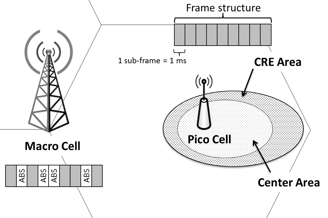
Figure 1: Illustration of Cell Range Extension and Almost Blank Sub-Frames in a HetNet

By setting a nonnegative $\text{CIO}_{dB}$ (CIO in dB) at the small BS we force the macro users to attach to a small cell which is not their best serving cell as shown in Figure 1. We say that these users are in the CRE area. Hence the CRE allows to increase the offloading of the macro cell. However, the CRE users now experience more interference from the macro BS which is their best serving cell. The macro cell interference reduces the SINR (SINR) at the CRE area thus limiting the extent of small cell offloading. The problem of interference mitigation for CRE users has been addressed by 3GPP and the ABS mechanism has been proposed.

II-A2 ABS

The ABS mitigation method consists in a time-domain interference avoidance. The goal is to reduce the interference from an aggressor cell (the cell causing the interference, which in our case is the offloaded macro BS) by almost blanking out some of its sub-frames as shown in Figure 1.

During the ABS, the aggressor cell mutes all of its traffic channels, leaving only certain control channels which are transmitted with reduced power. The ABS allows victim cells (namely the interfered small BS) to serve their users with almost no interference from the aggressor cell. The residual interference caused by the remaining control signals limits the gain from the ABS, and can be further mitigated using additional interference cancelation techniques introduced in 3GPP release 11 [13, Section 16.1.5].

It is advisable to schedule cell edge users during ABS because they are the most affected by interference. However, all the small cell users can benefit from ABS since their strongest interferer is generally a macro BS. The use of ABS decreases the available resources of the macro BS. Hence a trade-off should be found between the capacity gain of the small cells brought about the ABS and the corresponding capacity losses of the macro BS.

One may choose to schedule small cell UE in the CRE area exclusively during the ABS, and schedule the other small cell UE only during non-ABS. Alternatively, one may schedule all small cells’ UE during both ABS and non-ABS. We now discuss these two possible implementations.

II-B Implementation alternatives

II-B1 Protection of offloaded users

The first implementation for eICIC aims at protecting only the offloaded users at the CRE area of the small cells. Users of the small cells are divided into two groups: CRE users who are attached to the small cell due to the CIO, and center cell users who are attached to the small cell even when the CIO is set to $0$dB. The CRE users will be served by the small cell during the macro cell ABS. Note that this means a strictly positive CIO must be accompanied by a strictly positive ABSr, otherwise the users in the CRE area will never be served. We say that the two parameters (CIO and ABSr) are coupled.

Consider a CRE user $u$ and determine the SINR gain when he is offloaded from the macro cell to the small cell and is scheduled during ABS. Denote by the subscript $m$ the macro BS and by $p$ - the small BS. When attached to the macro BS $m$, user $u$ has a SINR equals to

$$S_{u,m}=\frac{h_{m}(u)P_{m}}{h_{p}(u)P_{p}+C_{0}(u)}$$ (2)

where $h_{m}(u)$ and $h_{P}(u)$ are the pathlosses from the macro cell $m$ to user $u$ and from the small cell $p$ to user $u$, respectively. $P_{m}$ and $P_{p}$ are the macro cell and small cell transmit powers, respectively. $C_{0}(u)$ is the total interference generated by the other nodes in the network (other macro BS and small BS) plus the thermal noise at the receiver of user $u$. If user $u$ is offloaded to the small BS and is served only during the ABS of macro cell $m$, then its SINR becomes

$$S_{u,m}=\frac{h_{p}(u)P_{p}(u)}{C_{0}(u)}$$ (3)

The SINR gain for this user can then be written as

$$\begin{split}SG_{u}&=\frac{h_{p}(u)P_{p}(h_{p}(u)P_{p}+C_{0}(u))}{h_{m}(u)P_{m}C_{0}(u)}\\ &=\frac{h_{p}(u)P_{p}}{h_{m}(u)P_{m}}+\frac{(h_{p}(u)P_{p})^{2}}{h_{m}(u)P_{m}C_{0}(u)}\end{split}$$ (4)

From equation (4) we can deduce the following simple condition on the received signals from the different BS at every point in the considered area for obtaining an offloading gain using ABS

$$\frac{(h_{p}(u)P_{p})^{2}}{h_{m}(u)P_{m}-h_{p}(u)P_{p}}>C_{0}(u)$$ (5)

If the condition (5) is not satisfied, offloading will result in performance degradation. Furthermore, there is a maximum CIO above which there is no gain for certain small cell users since as one gets further away from the small BS, $C_{0}(u)$ increases compared to the received signal strength from the small BS.

Condition (5) considers that only one macro cell implements ABS. If $M$ macro cells implement ABS, their interference will be removed from $C_{0}(u)$ so that condition (5) becomes

$$\frac{(h_{p}(u)P_{p})^{2}}{\sum_{m=1}^{M}h_{m}(u)P_{m}-h_{p}(u)P_{p}}>C_{0}(u)$$ (6)

which is verified for a larger number of CRE users.

We now give a simple example in which we can find at which extent a CRE can be performed, i.e. where offloading provides SINR gains. We consider a trisector macro cell site with one small BS in the coverage area of one of the macro sectors. To take into account neighbours’ interference, we add a tier of trisector macro sites to this cluster.

We focus on the SINR gains for users in the CRE area. By varying the number of macro BS applying ABS for the small cell users, we can see the evolution of the maximum CIO above which there is a SINR degradation at the edge of the small cells. The macros considered for muting are the most interfering ones.

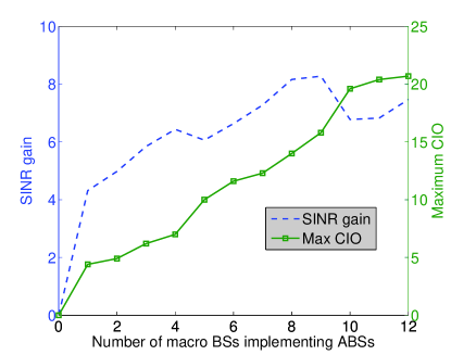
Figure 2: Maximum CIO for SINR improvement and SINR gain as a function of the number of macro BS applying ABS

Figure 2 presents the maximum CIO as a function of the number of macro BS providing ABS (red line with squares). It also shows the mean SINR gain obtained by the CRE users when setting the CIO to its maximum value (blue dashed line). The Figure illustrates condition (6), namely that muting more macro BS allows us to further increase the CIO. We can also see that the SINR gain obtained by muting more and more macro BS eventually saturates. Hence an optimal number of macro BS applying ABS can be found while keeping complexity low.

It is noted that if the small cells’ load is low, an offloading is still possible without applying the ABS which reduces the resources available for the macro cell. We present in the next section an implementation that allows to achieve this case.

II-B2 Protection of all small cell users

Instead of allowing only the CRE users to profit from ABS, in this implementation all the small cells’ users can benefit from the ABS, namely they can be scheduled during ABS or during normal sub-frames. In this case, offloading by increasing the CIO of the small cells without applying ABS is also allowed. We can say that the two parameters (CIO and ABSr) are decoupled. However if needed, the macro cell can provide ABS in order to enhance the offloading capability of the small cells. The SINR during ABS period is the same as that in the previous implementation. Only now, a small cell user will benefit part of the time from ABS and the rest of the time will experience normal SINR. The mean throughput of a macro user can then be written as

$$\bar{T}_{u,m}=(1-\theta)\bar{R}_{u,m}$$ (7)

where $\theta$ is the ABSr of macro $m$ and $\bar{R}_{u,m}$ - the mean data rate of user $u$ when it is served by macro cell $m$. The mean throughput of a small cell user is

$$\bar{T}_{u,p}=(1-\theta)\bar{R}_{u,p}^{\text{no ABS}}+\theta\bar{R}_{u,p}^{\text{ABS}}$$ (8)

where $\theta$ is the ABSr available to small cell $p$, $\bar{R}_{u,p}^{\text{no ABS}}$ and $\bar{R}_{u,p}^{\text{ABS}}$ are the average data rates of user $u$ over time when served by small cell $p$ outside and during the ABS respectively.

An efficient setting of the ABSr is needed to optimize a function of the users’ throughputs. A condition for achieving an offloading gain using ABS could be the increase of the total throughput of the considered cluster (macro cells and small cells)

$$\begin{split}&\sum_{m\in\mathcal{M}}\sum_{u\in m}(1-\theta)\bar{R}_{u,m}\\ &+\sum_{p\in\mathcal{P}}\sum_{u\in p}(1-\theta)\bar{R}_{u,p}^{\text{no ABS}}+\theta\bar{R}_{u,p}^{\text{ABS}}\\ &\geq\sum_{m\in\mathcal{M}}\sum_{u\in m}\bar{R}_{u,m}+\sum_{p\in\mathcal{P}}\sum_{u\in p}\bar{R}_{u,p}^{\text{no ABS}}\end{split}$$ (9)

where $\mathcal{M}$ and $\mathcal{P}$ are the set of all macro and small BS involved in the mechanisms (CRE and ABS).

Condition (9) may be too restrictive as we may want to increase the CET (CET) at the expense of a decrease in total throughput. In the next section, we propose self-optimization algorithms based on the two implementations described in this section, using a PF utility of UE throughputs as objective function.

III SON Algorithms

III-A Load Balancing SON

LB (LB) SON adjusts the small BS CIO in order to balance the loads between a macro BS and the small BS. The idea is to increase the small cell whenever its load is lower than that of the macro BS in the coverage area of which it is located (and vice versa). If we consider traffic offloading from macro $m$ to a small cell $s$, the ODE defining the LB SON mechanism at the small BS is defined by

$$\dot{CIO}_{{\text{dB}}_{s}}=\rho_{m}({\text{dB}}_{s})-\rho_{s}({\text{dB}}_{s})$$ (10)

where ${CIO_{\text{dB}}}_{s}$ is the CIO of small BS $s$ in decibels, $\rho_{m}$ - the load of the macro BS $m$, and $\rho_{s}$ - the load of the small BS $s$. The SA update equation defining the SON algorithm for (10) reads

$$CIO_{s}(k+1)=CIO_{s}(k)+\epsilon(\hat{\rho}_{m}(k)-\hat{\rho}_{s}(k))$$ (11)

where $\hat{\rho}_{m}$ and $\hat{\rho}_{s}$ are the estimators of $\rho_{m}$ and $\rho_{s}$ obtained by averaging the resource utilization of the respective BS over a certain time period. This SON converges to a set on which all loads are equal as shown in [12, Theorem 4].

In practice, a projected SA algorithm will be used instead of (11) because the CIO are restricted to a maximum value. The restriction is mainly due to the fact that offloaded users suffer from residual interference caused by remaining control channels during ABS. However, the convergence of the SA remains valid even in this case (see [11, §5.4]).

III-B ABS ratio optimization

We choose to implement the ABSrO (ABSrO) algorithm at the small BS which then requests appropriate ABSr from its interfering macro BS. The macro BS receives ABSr requests from the small cells it interferes and then applies the maximum ABSr among these requests. The ABSr optimization algorithm should then take into account load or traffic conditions (i.e. number of users present in the cell) of all the macro cells from which the considered small cell will be requesting ABS.

The cluster of BS considered for a single ABSrO algorithm comprises a small cell $p$ on which the algorithm is implemented, and the most interfering $M$ macro cells with small cell $p$. Typically $M=1$ is sufficient if the small cell is in the center of the macro cell, namely by periodically muting only one macro cell, we increase significantly the SINR of the small cell users. When the small cell is located at the cell edge, choosing $M=3$ provides better results.

III-B1 Only CRE users are protected

Using CRE, the small BS are able to offload traffic of the macro BS. The offloaded users at the small cell edge are highly interfered by the macro that previously served them. ABS are used to mitigate the interference enabling the small cells to offload even more the macro cell traffic.

The objective function considered in this implementation is the PF defined as follows

$$\begin{split}U_{PF1}(\theta)=&\sum_{m=1}^{M}\sum_{u\in m}\log((1-\theta)\bar{R}_{u,m})\\ +&\sum_{u\in\text{center of }p}\log((1-\theta)\bar{R}_{u,p}^{\text{no ABS}})\\ +&\sum_{u\in\text{CRE of }p}\log(\theta\bar{R}_{u,p}^{\text{ABS}})\end{split}$$ (12)

where we considered the $M$ most interfering macro BS users throughputs, the small cell center user throughputs and the small cell CRE area users throughputs. The PF utility enables us to maximize the users throughput and to enforce fairness among them. The SON algorithm applied to optimize this PF utility is given in the following theorem

Theorem 1.

Given some positive step sizes $\epsilon_{k}$ non-summable ($\sum_{k=0}^{\infty}\epsilon_{k}=\infty$) but square-summable ($\sum_{k=0}^{\infty}\epsilon_{k}^{2}<\infty$) and the update equation

$$\theta_{k+1}=\theta_{k}+\epsilon_{k}\left(\frac{N_{p,\textit{CRE}}}{\theta}-\frac{N_{p,\textit{CEN}}+\sum_{m=1}^{M}N_{m}}{1-\theta}\right)$$ (13)

where $N_{m}$, $N_{p,\textit{CEN}}$ and $N_{p,\textit{CRE}}$ are the mean numbers of active users in cell $m$, the center of cell $p$ and the CRE area of cell $p$, respectively,

then $\theta_{k}$ converges to a set on which $U_{PF1}()$ is maximal.

Proof.

See Appendix B. ∎

Note that the optimal $\theta$ can be directly derived in this case using (25) [7, Eq. 8], and is equal to

$$\theta^{*}=\frac{N_{p,\textit{CRE}}}{N_{p,\textit{CRE}}+N_{p,\textit{CEN}}+\sum_{m=1}^{M}N_{m}}$$ (14)

The reason we use a SA algorithm instead of setting optimal $\theta$ is to keep a certain stability in the parameter configuration which can be quite critical in real networks. Figure 3 illustrates this statement. Setting optimal ABSr at each event in the network (arrival or departure of a user) yields an extremely fluctuating parameter whereas the SA approach allows us to freeze the parameter at convergence when the traffic is stationary giving the same performance results.

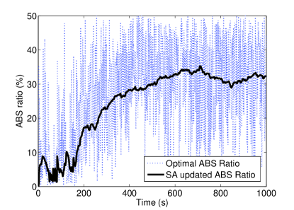
Figure 3: Time evolution of ABS ratio using stochastic approximation (solid line) and optimal solution (dashed line)

Performance results obtained using equation (13) are presented in Section IV. We now proceed with the second implementation for eICIC.

III-B2 All small cell users benefit from ABS

In this case, the user throughputs are modified according to equations (7) and (8).

The PF utility of the user throughputs is redefined as

$$\begin{split}U_{\text{PF2\_exact}}&(\theta)=\sum_{m=1}^{M}\sum_{u\in m}\log((1-\theta)\bar{R}_{u,m})\\ &+\sum_{u\in p}\log((1-\theta)\bar{R}_{u,p}^{\text{no ABS}}+\theta\bar{R}_{u,p}^{\text{ABS}})\end{split}$$ (15)

since we make no distinction between CRE users of the small cell and its normal users. The SON algorithm for optimizing the utility function (15) is presented in the following theorem.

Theorem 2.

Given some positive step sizes $\epsilon_{k}$ non-summable ($\sum_{k=0}^{\infty}\epsilon_{k}=\infty$) but square-summable ($\sum_{k=0}^{\infty}\epsilon_{k}^{2}<\infty$) and the update equation

$$\theta_{k+1}=\theta_{k}+\epsilon_{k}\left(\sum_{u\in p}\frac{1}{\theta_{k}+\frac{\bar{R}_{u,p}^{\text{no ABS}}}{\bar{R}_{u,p}^{\text{ABS}}-\bar{R}_{u,p}^{\text{no ABS}}}}-\frac{\sum_{m=1}^{M}N_{m}}{1-\theta_{k}}\right)$$ (16)

where $N_{m}$ is the mean number of active users in cell $m$,

then $\theta_{k}$ converges to a set on which $U_{\text{PF2\_exact}}()$ is maximal.

Proof.

See Appendix C. ∎

The update equation (16), requires the knowledge of the average data rates of all pico users, rendering practical implementation of the algorithm more complex. To simplify (16), we choose to maximize a lower bound of (15) instead. The new objective function is written as

$$\begin{split}U_{PF2}(\theta)=&\sum_{m=1}^{M}\sum_{u\in m}\log((1-\theta)\bar{R}_{u,m})\\ +&\sum_{u\in p}\frac{1}{2}\log(2(1-\theta)\bar{R}_{u,p}^{\text{no ABS}})\\ +&\sum_{u\in p}\frac{1}{2}\log(2\theta\bar{R}_{u,p}^{\text{ABS}})\end{split}$$ (17)

Lemma 1.

Let us consider $M$ macro cells and one small cell indexed $p$.

Then $\forall\theta\in]0,1[$ we have

$$U_{PF2}(\theta)\leq U_{\text{PF2\_exact}}(\theta)$$ (18)

Proof.

For the proof it suffices to show that for a small cell user $u$,

$$\begin{split}\log(2(1-\theta)\bar{R}_{u,p}^{\text{no ABS}})+\log(2\theta\bar{R}_{u,p}^{\text{ABS}})\\ \leq 2\log((1-\theta)\bar{R}_{u,p}^{\text{no ABS}}+\theta\bar{R}_{u,p}^{\text{ABS}})\end{split}$$ (19)

For ease of notation, denote $a=(1-\theta)\bar{R}_{u,p}^{\text{no ABS}}$ and $b=\theta\bar{R}_{u,p}^{\text{ABS}}$. We want to show that $\log 2a+\log 2b\leq 2\log(a+b)$. Using Jensen’s inequality [14] for the function $-\log$ which is convex we have

$$-\log\left(\frac{1}{2}(2a)+\frac{1}{2}(2b)\right)\leq-\frac{1}{2}\log(2a)-\frac{1}{2}\log(2b)$$ (20)

By taking the negative of (20), we obtain the desired result. ∎

The SON algorithm optimizing (17) is presented in the following theorem.

Theorem 3.

Given some positive step sizes $\epsilon_{k}$ non-summable ($\sum_{k=0}^{\infty}\epsilon_{k}=\infty$) but square-summable ($\sum_{k=0}^{\infty}\epsilon_{k}^{2}<\infty$) and the update equation

$$\theta_{k+1}=\theta_{k}+\epsilon_{k}\left(\frac{N_{p}}{2\theta_{k}}-\frac{\frac{N_{p}}{2}+\sum_{m=1}^{M}N_{m}}{1-\theta_{k}}\right)$$ (21)

where $N_{m}$ and $N_{p}$ are the mean numbers of active users in cells $m$ and $p$ respectively,

then $\theta_{k}$ converges to a set on which $U_{PF2}()$ is maximal.

Proof.

See Appendix D. ∎

The reasons for implementing a SA algorithm instead of setting the optimal ABS ratio (which can be easily derived) are the same as those stated in the previous section.

The SON algorithm (21) presents certain advantages over the one in (13). The first one is that we do not need to keep two counters for the numbers of active users of the small BS, but only one for the total number of users. The second one is that if the small BS has a very low load compared to those of its surrounding macro BS, the ABSr provided by those macro BS can be also low, thus preserving the resources of the macro BS. Furthermore, (21) is completely decoupled from the load balancing SON, whereas in (13), a positive CIO requires a corresponding ABSr. In the next section, we compare the performance results of the different SON algorithms.

IV Simulation Results

IV-A Simulation scenario

Consider a trisector BS surrounded by 6 interfering macro sites. In each macro sector 4 small BS are deployed close to the cell edge (see Figure 4). We consider elastic traffic where users arrive in the network according to a Poisson process, download a file and leave the network as soon as their download is complete. The considered area $A$ is the initial area covered by the macro - and the small BS. Two layers of traffic are superposed: the first one has a uniform arrival rate of $\lambda$ users/s all over $A$, and the second - a uniform arrival rate of $\lambda_{h}$ users/s in the initial area covered by the small cells (with all CIO set to 0dB). This is close to a realistic scenario where small cells are deployed in hotspot areas.

Following the SINR gain results presented in Figure 2, we choose three macro BS for ABSrO ($M=3$). Each small BS requests ABS from its three most interfering macro BS and take their load conditions (number of users to serve) into account in the ABSrO algorithms. To avoid truncation effects of the computational area in the simulations, we suppose that the surrounding macro BS serve 5 active users on the average.

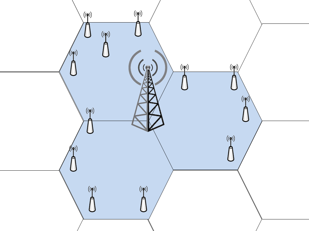
Figure 4: Network layout scenario

We use the propagation models for macro - and small BS (following [15, Page 61]) presented in Table I which also summarizes all the simulation parameters.

TABLE I: Network and Traffic characteristics

Network parameters
Number of macro BSs	3
Number of small BSs	12
Number of interfering macros	6 $\times$ 3 sectors
Macro Cell layout	hexagonal trisector
Small Cell layout	hexagonal omni
Intersite distance	500 m
Bandwidth	10MHz
Channel characteristics
Thermal noise	-174 dBm/Hz
Macro Path loss (d in km)	128.1 + 37.6 $\log_{10}(d)$ dB
small cell Path loss (d in km)	140.7 + 36.7 $\log_{10}(d)$ dB
Traffic characteristics
Traffic spatial distribution	uniform
$\lambda$	$\text{14 users/s/km}^{2}$
$\lambda_{h}$	$\text{6 users/s/km}^{2}$
Service type	FTP
Average file size	10 Mbits

IV-B Performance Evaluation

We first compare the performance using the exact PF utility function (16) and the approximate PF utility (21) for the second implementation (namely all small cell users can benefit from ABS). The results are presented in Figure 5 in terms of the Cumulative Distribution Function (CDF) of user throughputs. We can see that the exact utility (dashed blue line) gives slightly better MUT than the approximated PF utility (red stars curve), although the difference is not significant. We therefore consider in the following only the approximated algorithm (21), motivated by its much lower implementation complexity.

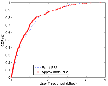
Figure 5: Comparison of user throughput CDF using the exact PF2 (21) - and the approximated PF2 (16) utility functions

We next compare the performance results for the following four cases:

1. Case 1: The initial network with no SON enabled, denoted hereafter as ’NoSON’. This case serves as a reference.

2. Case 2: The load balancing SON only, using algorithm (11), and denoted as ’LBonly’.

3. Case 3: The load balancing and ABSrO algorithms are enabled under implementation 1 of eICIC with ABSrO algorithm (13) using the PF utility function. This case is denoted as ’PF1’.

4. Case 4: The load balancing and ABSrO algorithms are enabled under implementation 2 of eICIC with ABSrO algorithm (21) using the approximated PF utility function. This case will be denoted as ’PF2approx’.

The chosen performance indicators are the global CET (Figure 7), the global MUT (Figure 8) and the maximum loads among the macro - and the small cells (Figure 6). The performance indicators are calculated over the coverage area of the 3 macro cells implementing the eICIC, which includes the 12 small cells.

Figure 6 shows that in all cases where SON is implemented, the loads are more or less balanced between macro cells (brown bars) and small cells (white bars). Interestingly, the ’LBonly’ case completely balances the loads since it is the only objective pursued in this case and the operating point where all the loads are balanced is feasible (the maximum CIO is not limiting). It is noted that in the ’PF1’ case, the increase of CIO is accompanied by the increase of ABSr of the interfering macro cells, resulting in higher loads than in the ’PF2approx’ case.

Figure 7 shows that eICIC in case ’PF1’ benefits the most to users with the worst SINR, namely provides the best CET, although the difference with case ’PF2approx’ is very small. The good CET performance of case ’PF1’ comes at the expense of a lower MUT, as shown in Figure 8. The highest MUT is provided by the ’LBonly’ case which better preserves macro cells’ resources (see Figure 8). However this comes at the expense of fairness, i.e. lower CET as shown in Figure 7.

The ’PF2approx’ case provides the best compromise between overall network capacity and fairness, namely between MUT and CET. All three cases implementing SON algorithms perform much better than the reference case with no SON and provide better QoS (QoS). Gain in CET is of 50%, 103% and 94% for ’LBonly’, ’PF1’ and ’PF2approx’ solutions respectively with respect to the reference ’NoSON’ solution. The gain in MUT is of 140%, 51% and 101% for ’LBonly’, ’PF1’ and ’PF2approx’ solutions, respectively, with respect to the reference ’NoSON’ solution. It is noted that only cases 3 and 4 (’PF1’ and ’PF2approx’) that implement each two SON functions can be considered as eICIC.

It is noticed that the performance gain of all algorithms presented in this paper depends on traffic density. For low traffic density, only the CET is enhanced while at high traffic density, all the KPI are improved by the SON functions. Hence in practice, a threshold related to traffic demand, e.g. the cell load, can be set to decide when to trigger the SON. Finally, it is noted that all SA based SON algorithms developed in the paper have fast convergence time, of the order of 20 minutes for stationary traffic.

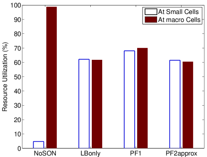
Figure 6: Comparison of the maximum loads among the macro - and small cells for cases 1–4

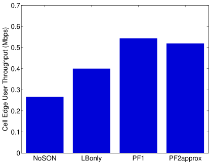
Figure 7: Cell Edge Throughput improvement for cases 1–4

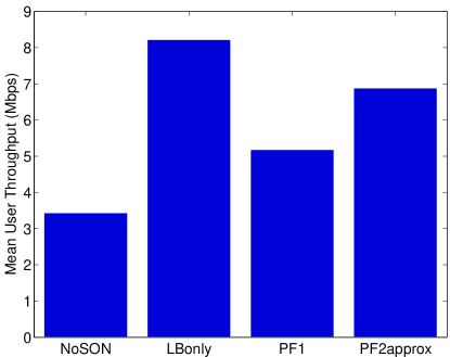
Figure 8: Mean User Throughput improvement for cases 1–4

V Conclusion and Remarks

In this paper we have investigated the problem of self-optimizing eICIC parameters, namely CRE and ABSr in LTE-Advanced heterogeneous networks. To this end, we have used results from SA which provide a powerful tool for designing simple and efficient SON algorithms. Fast convergence time is obtained for all the studied algorithms. The proposed eICIC SON comprizes two self-optimizing mechanisms. The first is a load balancing SON algorithm which adapts the CRE parameter of the small cells, and the second adapts the ABSr to maximize a PF utility of the user throughputs. Two possible implementations of the eICIC mechanism have been considered. The first implementation protects users in the cell edge of the small cells (CRE users) by scheduling them only during ABS of the neighboring macro BS. The second implementation allows all small cell users to benefit from the ABS mechanism. In each case, the appropriate ABSrO algorithm is provided. Performance results for a heterogeneous network with elastic traffic show that the second implementation of the eICIC mechanism provide better global results than the first one which only slightly outperforms in CET. So we can say that it is globally better to let all pico UE profit from ABS. In practice, an opportunistic scheduler such as PF can be used along with the second implementation of eICIC. Such implementation gives even more weight to the ’PF2approx’ algorithm which is expected to provide the best performance.

Appendix A Reminder on Stochastic Approximation

Let us consider a stochastic algorithm of the type

$$x_{k+1}=x_{k}+\epsilon_{k}(\nabla_{x}f(x_{k})+M_{k})$$ (22)

where $x\in\mathbb{R}$, $\epsilon_{k}\in\mathbb{R}^{+}_{*}$, $M_{k}$ is a noise value and $f()$ - a function we want to maximize. SA ([11, Theorem 2 P16]) says that if

• The series $\epsilon_{k}$ is non-summable; $\sum_{k=0}^{\infty}\epsilon_{k}=\infty$

• The series $\epsilon_{k}$ square summable; $\sum_{k=0}^{\infty}\epsilon_{k}^{2}<\infty$

• $M_{k}$ is a Martingale difference sequence with respect to the family of $\sigma$-fields $\Sigma_{k}=\sigma(x_{n},M_{n},n\leq k)$

• $\sup_{k}\|x_{k}\|<\infty$ almost surely

then $x_{k}$ converges to a compact connected internally chain transitive invariant set of

$$\dot{x}=\nabla f(x)$$ (23)

namely that the mean behavior of (22) is described by (23).

Appendix B Proof of Theorem 1

Suppose that the ABSr $\theta$ is bounded away from 0 and 1 ($\theta\in]0,1[$). Firstly, we can note that $U_{PF1}$ is differentiable on $]0,1[$ and let us evaluate its derivative. Using the properties of the log function ($\log(ab)=\log a+\log b$), we can rewrite $U_{PF1}(\theta)$ as

$$\begin{split}U_{PF1}(\theta)=&\sum_{m=1}^{M}N_{m}\log(1-\theta)+N_{p,\textit{CEN}}\log(1-\theta)\\ +&N_{p,\textit{CRE}}\log(\theta)+C_{1}\end{split}$$ (24)

where

$$\begin{split}C_{1}=&\sum_{m=1}^{M}\sum_{u\in m}\log(\bar{R}_{u,m})+\sum_{u\in\text{center of }p}\log(\bar{R}_{u,p}^{\text{no ABS}})\\ +&\sum_{u\in\text{CRE of }p}\log(\bar{R}_{u,p}^{\text{ABS}})\end{split}$$

is independent of $\theta$. From (24), we can easily derive

$$\frac{\partial U_{PF1}(\theta)}{\partial\theta}=\frac{N_{p,\textit{CRE}}}{\theta}-\frac{N_{p,\textit{CEN}}+\sum_{m=1}^{M}N_{m}}{1-\theta}$$ (25)

Using SA results (see Appendix A), we can see that the equivalent ODE to (13) is

$$\dot{\theta}=\frac{\partial U_{PF1}(\theta)}{\partial\theta}$$ (26)

Since $U_{PF1}(\theta)$ is the sum of the log of concave positive functions, it is concave. So (26) converges toward the maximum of $U_{PF1}(\theta)$.

Appendix C Proof of Theorem 2

The proof is similar to that of Theorem 1. Except now $U_{\text{PF2\_exact}}(\theta)$ is be rewritten as

$$\begin{split}U_{\text{PF2\_exact}}(\theta)=&\sum_{u\in p}\log((1-\theta)\bar{R}_{u,p}^{\text{no ABS}}+\theta\bar{R}_{u,p}^{\text{ABS}})\\ +&\sum_{m=1}^{M}N_{m}\log(1-\theta)+C_{2}\end{split}$$ (27)

where $C_{2}=\sum_{m=1}^{M}\sum_{u\in m}\log(\bar{R}_{u,m})$ is independent of $\theta$.

Function (27) is also a concave function of $\theta$ and its derivative reads

$$\frac{\partial U_{\text{PF2\_exact}}(\theta)}{\partial\theta}=\sum_{u\in p}\frac{1}{\theta+\frac{\bar{R}_{u,p}^{\text{no ABS}}}{\bar{R}_{u,p}^{\text{ABS}}-\bar{R}_{u,p}^{\text{no ABS}}}}-\frac{\sum_{m=1}^{M}N_{m}}{1-\theta}$$ (28)

The rest of the proof follows from Appendix B.

Appendix D Proof of Theorem 3

The proof is also similar to that of Theorem 1, except that $U_{PF2}(\theta)$ is written as

$$\begin{split}U_{PF2}(\theta)=&\sum_{m=1}^{M}N_{m}\log(1-\theta)+\frac{N_{p}}{2}\log(1-\theta)\\ +&\frac{N_{p}}{2}\log(\theta)+C_{3}\end{split}$$ (29)

where

$$\begin{split}C_{3}=&\sum_{m=1}^{M}\sum_{u\in m}\log(\bar{R}_{u,m})+\sum_{u\in p}\frac{1}{2}\log(\bar{R}_{u,p}^{\text{no ABS}})\\ +&\sum_{u\in p}\frac{1}{2}\log(\bar{R}_{u,p}^{\text{ABS}})+N_{p}\log(2)\end{split}$$

is independent of $\theta$.

Function (29) is also concave and its derivative will then be

$$\frac{\partial U_{PF2}(\theta)}{\partial\theta}=\frac{N_{p}}{2\theta}-\frac{\frac{N_{p}}{2}+\sum_{m=1}^{M}N_{m}}{1-\theta}$$ (30)

The rest of the proof follows from Appendix B.

References

- [1] 3GPP, “Evolved Universal Terrestrial Radio Access (E-UTRA) and Evolved Universal Terrestrial Radio Access (E-UTRAN); Overall description; Stage 2,” 3rd Generation Partnership Project (3GPP), TS 36.300 v10.11.0, Sep. 2013.
- [2] Y. Wang and K. I. Pedersen, “Performance analysis of enhanced inter-cell interference coordination in LTE-Advanced heterogeneous networks,” in Vehicular Technology Conference (VTC Spring), 2012 IEEE 75th. IEEE, 2012, pp. 1–5.
- [3] K. I. Pedersen, Y. Wang, B. Soret, and F. Frederiksen, “eICIC Functionality and Performance for LTE HetNet Co-Channel Deployments,” in Vehicular Technology Conference (VTC Fall), 2012 IEEE. IEEE, 2012, pp. 1–5.
- [4] M. Shirakabe, A. Morimoto, and N. Miki, “Performance evaluation of inter-cell interference coordination and cell range expansion in heterogeneous networks for LTE-Advanced downlink,” in Wireless Communication Systems (ISWCS), 2011 8th International Symposium on. IEEE, 2011, pp. 844–848.
- [5] J. Pang, J. Wang, D. Wang, G. Shen, Q. Jiang, and J. Liu, “Optimized time-domain resource partitioning for enhanced inter-cell interference coordination in heterogeneous networks,” in Wireless Communications and Networking Conference (WCNC), 2012 IEEE. IEEE, 2012, pp. 1613–1617.
- [6] A. Bedekar and R. Agrawal, “Optimal muting and load balancing for eICIC,” in Modeling & Optimization in Mobile, Ad Hoc & Wireless Networks (WiOpt), 2013 11th International Symposium on. IEEE, 2013, pp. 280–287.
- [7] S. Vasudevan, R. Pupala, and K. Sivanesan, “Dynamic eICIC—A Proactive Strategy for Improving Spectral Efficiencies of Heterogeneous LTE Cellular Networks by Leveraging User Mobility and Traffic Dynamics,” IEEE Transactions on Wireless Communications,, vol. 12, no. 10, pp. 4956–4969, 2013.
- [8] S. Deb, P. Monogioudis, J. Miernik, and J. P. Seymour, “Algorithms for Enhanced Inter-Cell Interference Coordination (eICIC) in LTE HetNets,” IEEE/ACM Transactions on Networking,, 2013.
- [9] Y. Khan, B. Sayrac, and E. Moulines, “Surrogate based centralized son: Application to interference mitigation in lte-a hetnets,” in IEEE 77th Vehicular Technology Conference (VTC Spring), 2013, pp. 1–5.
- [10] H. J. Kushner and G. G. Yin, Stochastic Approximation and Recursive Algorithms and Applications 2nd edition. Springer Stochastic Modeling and Applied Probability, 2003.
- [11] V. S. Borkar, Stochastic Approximation: A Dynamical Systems Viewpoint. Cambridge University Press, 2008.
- [12] R. Combes, Z. Altman, and E. Altman, “Self-organization in wireless networks: a flow-level perspective,” in Proceedings of IEEE INFOCOM, 2012.
- [13] 3GPP, “Evolved Universal Terrestrial Radio Access (E-UTRA) and Evolved Universal Terrestrial Radio Access (E-UTRAN); Overall description; Stage 2,” 3rd Generation Partnership Project (3GPP), TS 36.300 v11.7.0, Sep. 2013.
- [14] J. L. W. V. Jensen, “Sur les fonctions convexes et les inégalités entre les valeurs moyennes,” Acta Mathematica, vol. 30, no. 1, pp. 175–193, 1906.
- [15] 3GPP, “Evolved Universal Terrestrial Radio Access (E-UTRA); Further advancements for E-UTRA physical layer aspects,” 3rd Generation Partnership Project (3GPP), TS 36.814 v9.0.0, Mar. 2010.