SN 2011hs: a Fast and Faint Type IIb Supernova from a Supergiant Progenitor

Abstract

Observations spanning a large wavelength range, from X-ray to radio, of the Type IIb supernova 2011hs are presented, covering its evolution during the first year after explosion. The optical light curve presents a narrower shape and a fainter luminosity at peak than previously observed for Type IIb SNe. High expansion velocities are measured from the broad absorption H I and He I lines. From the comparison of the bolometric light curve and the time evolution of the photospheric velocities with hydrodynamical models, we found that SN 2011hs is consistent with the explosion of a 3–4 M_⊙ He-core progenitor star, corresponding to a main sequence mass of 12–15 M_⊙, that ejected a mass of ⁵⁶Ni of about 0.04 M _⊙, with an energy of $E=8.5\times 10^{50}$ erg. Such a low-mass progenitor scenario is in full agreement with the modelling of the nebular spectrum taken at $\sim$215 days from maximum. From the modelling of the adiabatic cooling phase, we infer a progenitor radius of $\approx$500–600 $R_{\odot}$, clearly pointing to an extended progenitor star. The radio light curve of SN 2011hs yields a peak luminosity similar to that of SN 1993J, but with a higher mass loss rate and a wind density possibly more similar to that of SN 2001ig. Although no significant deviations from a smooth decline have been found in the radio light curves, we cannot rule out the presence of a binary companion star.

1 Introduction

Core collapse supernovae (CC SNe) represent the final stage of the evolution of zero main sequence (ZAMS) massive stars $\ga 8M_{\odot}$ (Heger et al., 2003). SNe are generally classified on the basis of their early spectral appearance, which gives an indication on the nature of the evolutionary phase of the progenitor stars at the time of their explosion. The main division is defined by the presence or absence of hydrogen (H) lines, which splits CC SNe in Type II and Type Ib/c, respectively, and reveals whether or not the progenitor retained its H envelope before the explosion. An interesting group of CC SNe undergoes a peculiar spectral metamorphosis during their evolution: their spectra present at early phases broad H I absorption lines like a Type II SNe, which later disappear while He I features become predominant like in stripped envelope (SE) SN Type Ib spectra. For this reason, they are called Type IIb SNe.
The mechanism that explains how the progenitors of Type IIb SNe could shed most of the H layer at the time of explosion, while retaining enough mass ($\la$1 M_⊙; Nomoto et al. 1993) to show H signatures in their spectra is still under debate. The proposed scenario points to the explosion of a relatively high mass star ($\sim$ 25–30 M_⊙), which lost its H envelope by radiatively driven winds (Weiler et al. 2007; Stockdale et al. 2007; Smith & Conti 2008), or, alternatively, by mass transfer to a binary companion star (Yoon, Woosley, & Langer, 2010). A close binary companion could strip most of the external envelope also of a less massive star, allowing stars with a larger radius (like supergiant stars) to explode as Type IIb SNe (Eldridge, Izzard, & Tout 2008; Smith et al. 2011; Benvenuto, Bersten, & Nomoto 2013). In the extreme case of such a mass transfer, the companion could even spiral into the primary star and remove a large fraction of the envelope to form a single star progenitor of a Type IIb SN (Nomoto, Iwamoto, & Suzuki, 1995). Recently, it has been argued that a single star with an initial mass of 12–15 M_⊙ could explode as a Type IIb SN, if a much higher mass loss wind (up to 10 times) than the standard one (de Jager, Nieuwenhuijzen, & van der Hucht 1988; Mauron & Josselin 2011) is assumed, but the possible physical mechanism powering such a strong wind is still unidentified (Georgy 2012). So far, the wide variety in the observational properties of the small number of well-observed Type IIb SNe has made it impossible to favor a particular scenario among the possible ones.
SN 1987K was the first SN showing the Type II-Ib transition (Filippenko, 1988), although the most known and best studied Type IIb is SN 1993J (Filippenko, Matheson, & Ho 1993, Barbon et al. 1995, Richmond et al. 1996), considered the prototype of this class. The progenitor star of SN 1993J has been identified in pre-explosion images as a K-type supergiant in a binary system (Aldering, Humphreys, & Richmond 1994, Maund et al. 2004). Interestingly, a yellow supergiant (YSG) star was identified in pre-explosion images as the progenitor star of another well-studied Type IIb, SN 2011dh (Maund et al. 2011; Van Dyk et al. 2011; Arcavi et al. 2011; Marion et al. 2013; Sahu, Anupama, & Chakradhari 2013; Ergon et al. 2013), fully consistent with the numerical modelling of its bolometric light curve (Bersten et al. 2012), and definitely confirmed by the disappearance of the YSG candidate in post-explosion images taken almost two years after its explosion (Ergon et al. 2013; Van Dyk et al. 2013). Evidence of a binary companion has also been claimed for the Type IIb SN 2001ig (Ryder et al. 2004, 2006).
On the other hand, for the Type IIb SN 2008ax pre-explosion colours favour a bright stripped-envelope massive star with initial mass between 20–25 M_⊙, although the possibility of an interacting binary in a low-mass cluster could not be ruled out (Crockett et al. 2008; Chornock et al. 2011; Pastorello et al. 2008; Taubenberger et al. 2011).
Extensive data sets have been published for only a handful of Type IIb SNe, mainly due to the limited number of Type IIb SNe discoveries. This is the consequence of the intrinsic low rate (Type IIb SNe represent just 12% of the observed CC SNe; Li et al. 2011) and of possible misclassifications as Type Ib SNe, due to the strong dependence of the H lines strength on its mass/distribution and on the phase at which the SN is discovered (see Chornock et al. 2011; Stritzinger et al. 2009; Milisavljevic et al. 2013).
In this paper, we present the results obtained from the analysis of the data collected during the multi-wavelength followup campaign of the Type IIb SN 2011hs, located at R.A.=22^h57^m11$\aas@@fstack{s}{77}$ and Decl.=$-$43^∘23^′04$\aas@@fstack{\prime\prime}$08 (equinox 2000.0) at 20^′′ west and 41^′′north of the nucleus of the galaxy IC 5267. SN 2011hs was discovered on Nov. 12.5 (UT dates are used throughout the paper) with a 35-cm Celestron C14 reflector (+ ST10 CCD camera), at an unfiltered magnitude of 15.5 (Milisavljevic et al., 2011). Our observational campaign started immediately after the announcement of the discovery, sampling the SN evolution in a wide wavelength range, spanning from the X-ray to the radio domain. The first optical spectrum obtained on Nov. 14.9 with the 10-m SALT telescope (+RSS), revealed that SN 2011hs was a Type IIb SN, with a H$\alpha$ expansion velocity resembling the fast expanding Type IIb SN 2003bg (Milisavljevic et al., 2011).
X-ray and ultraviolet (UV) observations of SN 2011hs were secured with the Swift (Gehrels et al., 2004) satellite from Nov. 15 until the SN faded below the detection threshold.
We intensively monitored the optical and near-infrared (NIR) spectrophotometric evolution of SN 2011hs out to $\sim 65$ days past the discovery, when the campaign was suspended because of the SN conjunction with the Sun, and then restarted in April 2012 and continued until 2012 Oct. 22, the epoch of the last observation published here. The presented optical/NIR dataset is the outcome of the coordination of various observing programs at different telescopes in different observatories located in Chile [Las Campanas Observatory (LCO), ESO La Silla Observatory and Cerro Tololo Interamerican Observatory (CTIO)] and South Africa (Southern African Astronomical Observatory).
Radio monitoring of SN  2011hs with the Australia Telescope Compact Array (ATCA) began within a week from its discovery, collecting multi-frequency radio flux data for the first 6  months at frequencies between 1 and 20  GHz.
The paper is organized as follows: the photometric and spectroscopic observations are presented in Section 2, where the observational campaign and methods for data reduction for each wavelength range are described. In Section 3, we define the host galaxy properties, i.e. distance and dust extinction, while in Section 4 and Section 5 we analyze the photometric and spectroscopic evolution of the SN. In Section 6, we present the hydrodynamical modelling performed to estimate physical parameters of the SN progenitor and its explosion. Section 7 deals with the radio data modelling and, finally, in Section 8 we summarize the results and present our conclusions.

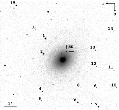
Figure 1: SN 2011hs in IC 5267 and the sequence of local reference stars (cf. Table 2 and 3). The image is a $V$ frame taken with PROMPT on 2011 Nov 19.

2 Observations

2.1 X-Ray Observations

Swift-XRT (Burrows et al., 2005) observations were acquired starting from Nov. 15.3 to Nov. 26.3, for a total of 31.3 ks. HEASOFT (v. 6.12) package has been used to calibrate and analyze Swift-XRT data. Standard filtering and screening criteria have been applied. We find evidence for X-ray emission originating from the host galaxy nucleus at the level of $\sim(2.2\pm 0.2)\times 10^{-13}\,\rm{erg\,s^{-1}cm^{-2}}$ (unabsorbed flux in the 0.3-10 keV energy band). As reported in Margutti, Soderberg, & Milisavljevic (2011), no significant X-ray emission is detected at the SN position, with a 3 sigma upper limit of $1.3\times 10^{-3}\,\rm{c\,s^{-1}}$ (0.3-10 keV band). The Galactic neutral hydrogen column density in the direction of the SN is $1.22\times 10^{20}\,\rm{cm^{-2}}$ (Kalberla et al., 2005). Assuming a spectral photon index $\Gamma=2$, this translates into an unabsorbed upper limit flux $F<6.4\times 10^{-14}\,\rm{erg\,s^{-1}cm^{-2}}$, corresponding to a luminosity $L<5.2\times 10^{39}\,\rm{erg\,s^{-1}}$ at the assumed distance of 26.4 Mpc (see Sect. 3). The presence of an extended X-ray emission from the host galaxy nucleus and the proximity of SN 2011hs to the nucleus (compared with the Swift-XRT PSF) prevents us from providing a deeper limit. In any case, considering the X-ray luminosities observed in previous studied Type IIb SNe, we can conclude that a SN like SN 2011dh, with a $L_{X[0.3-8keV]}\approx 1.5\times 10^{38}\,\rm{erg\,s^{-1}}$ (Soderberg et al., 2012) would not have been detected, whilst SN 1993J, with a luminosity of $L_{X[0.3-8keV]}\approx 8\times 10^{39}\,\rm{erg\,s^{-1}}$, would stand out on the background.

2.2 UVOT Observations

Swift-UVOT (Roming et al., 2005) data were acquired using the 6 broad-band filters (w2, w1,m2, u, b and v), spanning a wavelength range from $\lambda_{c}=1928$ Å (w2 filter) to $\lambda_{c}=5468$ Å (v filter). Data have been analyzed following the prescriptions of Brown et al. (2009). In particular, a 3^′′ aperture has been used to maximize the signal-to-noise ratio and limit the contamination from host galaxy light. We removed the residual contamination from host galaxy light selecting a number of background regions close to the SN site (unfortunately, no UVOT pre-explosion images of SN 2011hs are available). Swift UV and optical photometry, based on the UVOT photometric system of Poole et al. (2008), is reported in Tabs. 1 and 4.

2.3 Optical and NIR Photometry

The optical photometric follow up of SN 2011hs was almost entirely obtained with the 0.41m Panchromatic Robotic Optical Monitoring and Polarimetry Telescope (PROMPT; Reichart et al. 2005) and the 50cm CATA500 Telescope, both located at the CTIO, which offered BVRI+u^′g^′r^′i^′z^′ and BV+u^′g^′r^′i^′ coverage, respectively. Additional optical (UBVRI) data were acquired at the du Pont Telescope, a 2.5m-class telescope at LCO, using the Wide Field Reimaging CCD Camera (WFCCD), and at the 3.6m ESO New Technology Telescope (NTT), mounted with the ESO Faint Object Spectrograph and Camera 2 (EFOSC2). The last nebular $BVRI$ epoch was acquired at the ESO Paranal Observatory with the Very Large Telescope Unit 1 (VLT/UT1) equipped with the FOcal Reducer/low dispersion Spectrograph 2 (FORS2). For optical images, standard reductions were performed using IRAF tasks, including bias and flat-field corrections. A point-spread-function (PSF) fitting method was applied to measure the SN magnitudes. Since the background at the SN position is fairly regular, we did not need to perform a template subtraction, and thus we removed its contribution to the SN flux evaluating it by means of a two-dimensional low-order polynomial fit of the region surrounding the SN. SN 2011hs instrumental magnitudes were calibrated to the standard Johnson–Cousins and Sloan photometric systems using the relative colour equations, obtained for each instrument observing Landolt (2007) and Smith et al. (2002) standard star fields over the course of photometric nights. We also measured and calibrated the magnitudes of a local sequence of stars, whose positions in the field are shown in Fig.1. Magnitudes were computed via a weighted average of the measurements made during the photometric nights (3 nights for $UBg^{\prime}$ bands and 6 nights for the remaining ones) and reported in Tables 2 and 3. We used the magnitudes of the local stars sequence to obtain the photometric zero-points for non-photometric nights. Because of the small field of view and of the faintness of the local field stars, only one star was available for the calibration of the U-filter images.
During the very early phases unfiltered images were collected by amateur astronomers of the Backyard Observatory Supernova Search (BOSS) project. We included BOSS observations performed on Nov. 12.5 (used for the discovery; Milisavljevic et al. 2011) and Nov 14.15 and 14.16 in our analysis. Since the quantum efficiency of the employed CCD peaks around 6500 Å, we calibrated the unfiltered magnitudes as Johnson-Bessell $R$ band images. In addition, by using the local stars sequence we estimated a color correction, which turned out to be quite small ($<$20% of the ($V-R$) colour) and corresponding to a negligible correction for the SN $R$ band magnitudes ($\sim 0.02-0.03$ mag).
NIR photometry was acquired, using a variety of facilities, including JHK images with the SOFI camera mounted at NTT; JH images with the NIR camera of the robotic 60-cm telescope REM in LaSilla; and finally, JH images with the RetroCam at the DuPont telescope. The images from each instrument were calibrated using field stars from the Two Micron All-Sky Survey (2MASS). SN 2011hs magnitudes are tabulated in Tables 4, 5 and 6, where the uncertainties are a quadratic sum of the errors of the instrumental SN magnitude measurement and the photometric calibration.

2.4 Optical and NIR Spectroscopy

The log of the 24 spectroscopic epochs we obtained is reported in Table 7. In addition to the telescope/instruments used also for the photometry (and described in Sect. 2.3), optical spectra were taken at: the Southern African Large Telescope (SALT) with the Robert Stobie Spectrograph (RSS); the Magellan Telescope (+ LDSS3) at LCO; and the SOAR(+Goodman Spectrograph) Telescope on Cerro Pachon. NIR spectra were obtained at NTT+SOFI and at the Magellan Telescope + FIRE spectrograph.
Spectra were reduced using IRAF tasks, within noao.onedspec and ctioslit package. Spectrophotometric (Hamuy et al. 1992, 1994) and telluric standard-star exposures taken on the same night as the SN 2011hs observations were used to flux-calibrate the extracted spectra and to remove telluric absorption features, respectively. We checked the flux calibration of the spectra against the simultaneous broad-band photometry and, if required, the spectrum was rigidly scaled to match the photometry. The simultaneous spectra obtained at Magellan(+IMACS) and at the du Pont Telescope (+WFCCD) on Nov. 18th (see Table 7) were combined and presented as a single spectrum.

2.5 Radio Observations

SN 2011hs follow-up at the radio wavelength range (2.0-18.0 GHz) was performed at the Australia Telescope Compact Array (ATCA) and started from Nov 17.4 UT. The total time on-source ranged from 1 to 3 hours, yielding sufficient $uv$-coverage to comfortably resolve SN  2011hs from the nucleus of IC  5267 ($45\arcsec$ to the south-east). Table 8 contains the complete log of observations and radio flux measurements from the ATCA, where epochs are given as days elapsed since the discovery. The Compact Array Broad-band Backend (CABB; Wilson et al. 2011) provides $2\times 2$  GHz IF bands, each of which has $2\times 2048$ channels of 1  MHz each. The first 2 epochs covered the frequency bands of 4.5–6.5  GHz and 8.0–10.0  GHz; the next 5 epochs also included the bands 16.0-18.0  GHz and 18.0–20.0  GHz; while the final 3 epochs replaced these highest frequency bands (where the SN was no longer detectable) with both IFs now covering 1.1–3.1  GHz.
The ATCA primary flux calibrator, PKS  B1934-638 was observed once per run at each frequency to set the absolute flux scale. It also defined the bandpass calibration in each band, except for 18  GHz where the brighter source PKS  B1921-293 was used instead. Frequent observations of the nearby source PKS  B2311-452 allowed us to monitor and correct for variations in gain and phase during each run, and to update the antenna pointing model at 18  GHz.

The data for each observation and separate IF band have been edited and calibrated using tasks in the miriad software package (Sault et al., 1995). The large fractional bandwidths used enable “multi-frequency synthesis”, in which $uv$-plane coverage is improved by gridding each channel individually, followed by multi-frequency deconvolution of the dirty image to account for the spectral index of each source. Despite this the factor of 3 change in beam size over the 1.1–3.1 GHz band, coupled with the significant amount of interference wiping out the lower 512 MHz of this band, required its splitting into two sub-bands of 768 MHz, centered on 2.0 GHz and 2.7 GHz.

Robust weighting was employed in the imaging to give the best compromise between the minimal sidelobes produced by uniform weighting, and the minimal noise achieved with natural weighting. While Gaussian fitting of the clean beam to an unresolved source is a standard way of determining the flux of a radio point source, at low flux levels fitting to the calibrated visibilities in the $uv$-dataset can be more reliable. The UVFIT task has been used to fit simultaneously a point source at the known location of SN 2011hs, as well as the nearby nucleus of the host galaxy IC 5267, which was of comparable but more stable luminosity than SN 2011hs. Following Weiler et al. (2011) the uncertainties in Table 8 are the quadrature sum of the image rms and a fractional error on the absolute flux scale in each band.

3 Distance and dust extinction

The adopted distance for SN 2011hs is based on the recession velocity value obtained from the accurate folding of the stellar velocity rotation curve (Morelli et al., 2008). We derived a recession heliocentric velocity of 1710 $\pm$ 20  km s^-1, in excellent agreement with the tabulated value in the NED catalog (Koribalski et al., 2004). Corrected for the peculiar solar motion (Kerr & Lynden-Bell, 1986), this corresponds to a redshift equal to z = 0.0057 $\pm$ 0.0001 and a distance modulus $\mu=31.85\pm 0.15$ mag (where Hubble constant H₀= 73   km s^-1 Mpc^-1, $\Omega_{\Lambda}$=0.73 and $\Omega_{M}$=0.27). On the other hand, from the early time SN 2011hs spectra, we measured an average shift of the H$\alpha$ central wavelength corresponding to a recession heliocentric velocity of 1910 $\pm$ 40 km s^-1, 200 km s^-1 higher than the galaxy nucleus. This is consistent with the values obtained from the velocity rotation curve of the gas ([N II] line) component at a radius of 45 arcsec along the major axis of the galaxy. The data reduction and analysis used to extract the gas kinematic are described in Morelli et al. (2008) and Morelli et al. (2012). The gas and stellar kinematic for this S0 galaxy unveiled a very peculiar and interesting structure, with the inner (r$<$ 5 arcsec) region of the galaxy rotating in the opposite direction with respect to its external region (as seen in e.g. NGC 4826, Rubin 1994). The kinematics of the stellar and gas components show the same radial trend, although the values of the stellar and gas velocity do not match in the disk dominated region, being $<$30 km s^-1 and $>$100 km s^-1, respectively. This suggests that the face on stellar component is not aligned with the gas components, probably due to a strong warp in the radial structure of the gas disk or to a different inclination of stellar and gas disks. It is not obvious how to associate the SN to either the stellar or the gaseus component and decide which velocity correction to apply to our spectra. Nevertheless, considering that the $\Delta$v$\sim$200 km s^-1 with respect to the nucleus value would result in a wavelength offset of $\sim$4 Å (which is much greater than the $\sim$1–2 Å  uncertainty affecting the spectral wavelength calibration), we found that by applying the shift found from the H$\alpha$ emission, the maxima of the forbidden emission lines in the nebular spectra (see Sect. 5.3) fall at the proper rest-frame wavelengths. Thus a recession velocity of $v$=1910 $\pm$ 40 km s^-1 will be employed for the analysis in this paper.
For the Milky Way extinction we used the IR maps by Schlafly & Finkbeiner (2011), that give for our observing direction an $E(B-V)_{\rm MW}=0.011\pm 0.002$ mag. On the other hand, the estimation of the extinction due to the host galaxy dust is a tricky issue, and is a considerable source of systematic uncertainty in SN studies. A proxy for host galaxy reddening is given by a correlation that links the column density of neutral sodium (Na) with the absorption and scattering properties of dust, using the equivalent width (EW) of the interstellar Na I D absorption doublet ($\lambda\lambda$5890, 5896 Å; Turatto, Benetti, & Cappellaro 2003; Poznanski, Prochaska, & Bloom 2012). We estimated EW(Na I D) from the first spectrum ($-$5 days) to 10 days after the $B$-maximum light (hereafter $t(B)_{max}$), when He I lines started to dominate the spectrum (cf. Sec. 5). We observed a high scatter of the EW(Na I D) measurements, although it did not show any trend. Thus we adopt an average value EW(Na I D)= 0.90$\pm$0.19 Å (with the error given by the rms of the distribution). Applying the relation by Poznanski, Prochaska, & Bloom (2012), $log(E(B-V))=1.17\times{\rm EW(Na\,I\,D)}-1.85\pm 0.08$, we obtain an $E(B-V)_{\rm host}=0.16\pm 0.07$ mag. As a comparison, applying the relation by Turatto, Benetti, & Cappellaro (2003), ${\rm E(B-V)=0.16\times EW(Na\,I\,D)}$, an E(B-V)=0.14$\pm$0.03 mag is obtained, in agreement with the previous value. Thus the total (Milky Way + host galaxy) color excess value adopted throughout this work is $E(B-V)_{tot}=0.17\pm 0.08$ mag.

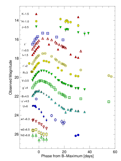
Figure 2: Early-phase light curves of SN 2011hs extending from the UV to the NIR wavelengths. Observed magnitudes are not corrected for reddening and vertically shifted for clarity of the plot. The epochs are computed with respect to the $t(B)_{max}$, i.e. Nov. 20 (2,455,885.5 $\pm$ 1.0 JD). The filter name corresponding to each light curve is reported on the left side. Swift/UVOT u, b and v magnitudes are reported with small symbols.

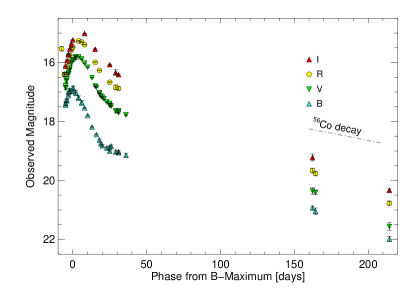
Figure 3: Time evolution of SN 2011hs in BVRI bands through the nebular phases.

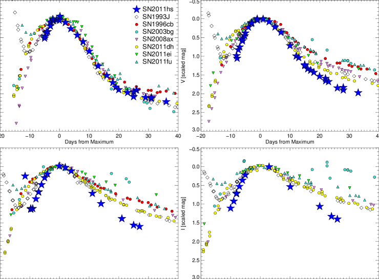
Figure 4: Comparison of SN 2011hs BVRI light curve shapes with those of SNe 1993J (Barbon et al. 1995; Richmond et al. 1996); 1996cb (Qiu et al., 1999); 2003bg (Hamuy et al., 2009); 2008ax (Pastorello et al. 2008; Taubenberger et al. 2011); 2011dh (Ergon et al., 2013); 2011ei (Milisavljevic et al., 2013); 2011fu (Kumar et al., 2013). The phase is computed with respect to the relative maximum light.

4 the Light curves

Light curves of SN 2011hs obtained in the different bands from UV to the NIR wavelength range are shown in Figs. 2 and 3. The follow up spans epochs from 2011 Nov. 14.5 to 2012 Jan. 16.1 for most of the filters, with the exception of BVRI bands for which it was extended to 2012 Jun. 20.4 UT. As described also in Section 6, Type IIb SN light curves are expected to be characterized by an initial decline, as a consequence of the adiabatic cooling of the ejecta after the shock breakout (see e.g. Woosley et al. 1994; Blinnikov et al. 1998; Bersten et al. 2012). Such a cooling phase has been observed in very few Type IIb SN cases: i.e. SNe 1993J (Barbon et al. 1995; Richmond et al. 1996), 2011dh (Arcavi et al., 2011) and, recently, 2011fu (Kumar et al., 2013). The cooling branch is followed by a rising to a peak, powered by the radioactive decay of the ⁵⁶Ni, produced during the explosion, and its daughter ⁵⁶Co. Assuming that SN 2011hs followed the same path, it appears that the observational campaign started when the SN was already in the post-cooling rising phase (Fig. 2). Indeed early photometry based on the amateur discovery image shows that SN 2011hs initially decreases by 0.88 mag ($R$ band) in 1.9 days. Such a first point, as shown in Sect. 6, aids us in constraining the light curve modelling and, thus, determining the progenitor star radius at the time of the explosion.
For the bands with a more detailed sampled light curve, we estimated the epoch of the peaks and their magnitude using low order polynomial fits. These are reported in Table 9, along with the pre- and post-maximum light curve slope estimations obtained using least-squares fits.
SN 2011hs reached $t(B)_{max}$ on 2011 Nov. 20 (corresponding to 2,455,885.5 JD), while light curves in redder filters peak some days later. As shown in Fig. 4, SN 2011hs has the steepest rise to the peak among the Type IIb SN sample we found in literature (i.e. SNe 1993J, Barbon et al. 1995, Richmond et al. 1996; 1996cb, Qiu et al. 1999; 2003bg, Hamuy et al. 2009; 2008ax, Pastorello et al. 2008, Taubenberger et al. 2011; 2011dh, Ergon et al. 2013; 2011ei, Milisavljevic et al. 2013; 2011fu, Kumar et al. 2013).
This is true also for its post-maximum decline in the $VRI$ bands (e.g. for the I band SN  2011hs has a rate of 0.07$\pm$0.01 mag d^-1, while it is 0.05$\pm$0.01 mag d^-1 and 0.02$\pm$0.01 mag d^-1 for SN 1993J and SN 2011fu, respectively; see Table 5 in Kumar et al. 2013), while in the $B$ band (0.09$\pm$0.01 mag d^-1) it is similar to that of the other Type IIb SNe (e.g. 0.11$\pm$0.01 mag d^-1 and 0.10$\pm$0.01 mag d^-1 for SN 1993J and SN 2011fu, respectively, from Table 5 in Kumar et al. 2013).
Adopting the distance modulus and reddening discussed in Section 3, we find a B and V absolute peak magnitude of $-15.63$ mag and $-16.59$ mag, respectively. A comparison among a sample of Type IIb SN absolute light curves is shown in Fig.  5. SN 2011hs appers to be the faintest Type IIb SN in the B band, while in the $V$ band turns out to be as bright as SN 1996cb. This results in a high $(B-V)$ colour value as shown in the next section (Sect. 4.1).
SN 2011hs nebular photometry was obtained only in the BVRI bands, as shown in Fig. 3. From it, we measured a slope of $2.31\pm 0.28$ mag (100d)^-1 in the $V$ band, which is steeper than the rate expected for ⁵⁶Co decay in the case of complete $\gamma$-ray trapping (0.98 mag/100d). This is commonly found in SE SNe at nebular phase (100-300 days after maximum) and it is attributed to rather low ejecta masses with respect to SNe IIP (Clocchiatti & Wheeler, 1997).

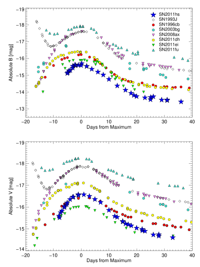
Figure 5: Comparison of the $B$ (upper panel) and $V$ band (lower panel) absolute magnitude light curves of SN 2011hs compared with those of the sample of SNe Type IIb presented in Figure 4.

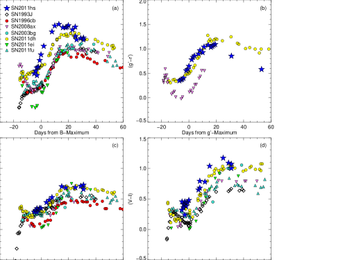
Figure 6: Comparison of SN 2011hs colour curves with those of the sample of SNe Type IIb presented in Figure 4. All the colour curves are corrected for the relative reddening value.

4.1 Colour Evolution

In Fig. 6, we show the evolution of ($B-V$), ($g^{\prime}$-$r^{\prime}$), ($V-R$) and ($V-I$) intrinsic colour of SN 2011hs (colour excess used $E(B-V)=0.17$ mag; see Sect. 3) and compare them with those of the same Type IIb SNe sample, corrected for the relative reddening value. In general, SN 2011hs shows redder colours and more rapid evolution than the comparison SNe. In particular, the ($B-V$) colour evolution of most of the Type IIb SNe follow that of SN 2008ax, that after an initial move to blue colour, starts getting redder with an initial rise of $\sim$0.03 mag d^-1 from -5 days to 5 days, which then becomes steeper (with a rate of 0.056$\pm$0.004 mag d^-1) until about two weeks after maximum. Only few SNe differ from this behaviour: i.e. SNe 1993J and 2011fu, which start with bluer colours at very early phases post-explosion, evolve monotonically to red colours, but already after $-$10 days from maximum follow the average trend, and SN 2011ei, whose initial rise to red colours has a steeper slope. The SN 2011hs ($B-V$) colour curve (which at maximum light has an offset $\Delta(B-V)\sim$0.6 mag from SN 2008ax) displays a peculiar evolution: it shows an initial increase with a rate of 0.061$\pm$0.003 mag d^-1 between -5 days and 15 days, similar only to SN 2011ei ($\Delta(B-V)/\Delta$t = 0.061$\pm$0.004 mag d^-1 in the same time interval); later, during the decline to bluer color, at about one month from $t(B)_{max}$, the colour undergoes a drop of $\sim$0.2 mag in one day. Following this, the SN 2011hs colours become similar to those of the other Type IIb SNe. In contrast, the $(V-R)$ and $(V-I)$ colour evolution of SN 2011hs do not differ significantly from those of the other Type IIb SNe. Similarly to SN 2011dh, SN 2011hs ($g^{\prime}-r^{\prime}$) colour is characterized at maximum light by a $\Delta(g^{\prime}-r^{\prime})\sim$0.5 mag with respect to SN 2008ax, but it has a much steeper slope to bluer colours during the late stages of its evolution.
The redder colours showed by SN 2011hs could point to an underestimation of the reddening effect. It is common practice in SN studies to estimate the host galaxy extinction through the colour excess measured by comparing the colour curve of the SN to a “template” curve, which is basically obtained by averaging the colour curves of SNe belonging to the same SN class. This method is based on two assumptions: firstly that there is a similarity among the intrinsic colour evolutions of SNe of the same class and, secondly, that those SNe used to construct the template curve are affected by a negligible reddening. SN 2003bg is the only object in the well studied Type IIb SN sample that is assumed to have a no significant extinction from the host galaxy, since its spectra do not show Na I D absorption lines (Hamuy et al., 2009). Unfortunately, we lack of a photometric coverage from about the maximum light epoch to 20 days later. This prevents us to use it as a template, since we cannot ensure that its colour curve shape was similar to that of SN 2011hs. Nevertheless, we found a good agreement between the two SNe at the common epochs, which makes us confident of the reddening correction adopted. As we reported here, SN 2011ei had a colour evolution similar to SN 2011hs, so it could be considered a good template. However, it shows to be much bluer that the other Type IIb SNe (see Fig. 6) and, most importantly, its reddening was estimated through the Na I D method too. Therefore, by using it, we actually could introduce an additional source of uncertainty in our reddening estimation. Thus this method cannot be applied in order to disentangle the possible effects of the reddening from those of a different intrinsic SN colour (due to e.g. a different SN temperature) at least until a sample of unreddened Type IIb SNe will be assembled.

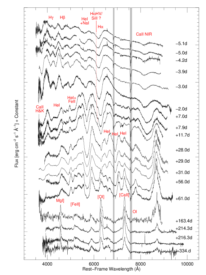
Figure 7: Spectroscopic sequence of SN 2011hs ranging from $-5.1$ to +334.0 days after $t(B)_{max}$. Each spectrum has been reported to the host galaxy rest frame, corrected for Milky Way and host galaxy reddening and, finally, shifted by an arbitrary amount for presentation. On the right, the phase from $t(B)_{max}$ are labeled. Grey bands indicate the telluric bands position.

5 Spectral Evolution

Fig. 7 contains the spectral sequence of SN 2011hs, ranging from about 5 days before $t(B)_{max}$ to about one year later (334 days). At the earliest phases, the spectra are dominated by the H Balmer series lines, with the typical P-Cygni profile. From the minimum of the absorption components, we measured an expansion velocity around 17,000 km s^-1 for H$\alpha$, and 14,000 km s^-1 for H$\beta$ and H$\gamma$, with the latter being slower because of a higher optical transparency of the ejecta at these wavelengths. Absorption features at $\sim$4300 Å and $\sim$5600 Å are identified as He I lines $\lambda\lambda$4472 and 5876, respectively, with the latest likely blended with Na I. The broad absorption feature at $\sim$8200 Å  is due to the Ca II NIR triplet. Ca II H&K absorption at around 3750 Å is also present. Evolving through maximum, the strength of H$\alpha$ changes, as well as its profile, with the emergence of a shoulder in the blue-wing, clearly detectable around one week after maximum. As recently discussed by Hachinger et al. (2012), this line (see Figures 7 and 8) could be identified as Si II, moving at early phases at about 12,000 km s^-1 in SN 2011hs case, or as H$\alpha$ emission from a high velocity H bubble with a velocity of $\sim$20,000 km s^-1. In the latter case, we would expect to detect such high velocity components also in the H$\beta$ and H$\gamma$. Indeed, while near H$\gamma$ the S/N is too low for a detailed analysis, H$\beta$ seems to show a hint of a double minimum profile in the spectra between -4 and -3 days from maximum with a possible high velocity component at $\sim$14,500 km s^-1. However, we cannot discard the identification of these features with other ions, i.e. Co II or Fe II, as modeled by Mazzali et al. (2009) and, recently, by Hachinger et al. (2012).
A week after maximum, the spectrum is dominated by strong absorptions of He I, with the features at around 6550, 6900 and 7200 Å becoming more conspicuous and identified as He I $\lambda\lambda$6678, 7065 and 7281, respectively. These lines become dominant within one month after the maximum, whilst in the blue part of the spectrum, Fe II lines emerge.
We followed the spectral evolution of the SN until its Sun conjunction, two months after $t(B)_{max}$. When the SN became visible again, we obtained a nebular phase spectrum (+163 day), which displays the typical emission features of a SE SN, i.e. prominent Mg I] $\lambda$4570, [O I] $\lambda$5577, [O I] $\lambda$$\lambda$6300, 6363 and [Ca II] $\lambda$$\lambda$7291,7324 emission lines. The [Fe II] emission at $\sim$5200 Å appears faint, suggesting that a small amount of ⁵⁶Ni is produced in the explosion. Finally a boxy feature redwards of the [O I] line at $\sim$6600 Å  is present and strengthens with time. Nebular line profiles are discussed in Sects. 5.3 and 5.2.

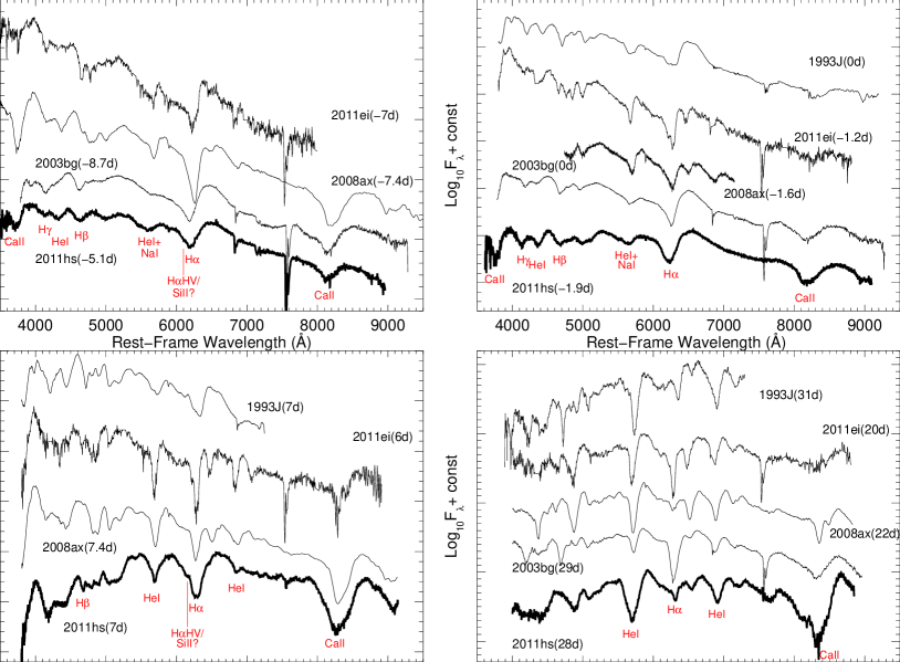
Figure 8: Comparison of SN 2011hs spectra with those of Type IIb SNe 1993J (Barbon et al. 1995; Richmond et al. 1996), 2008ax (Pastorello et al. 2008; Taubenberger et al. 2011), 2011ei (Milisavljevic et al., 2013) and 2003bg (Hamuy et al., 2009), at similar phases after $t(B)_{max}$, namely around $-$7 days (upper left panel), 0 days (upper right panel), 7 days (lower left panel) and 30 days (lower right panel). Spectra have been corrected for total (Milky Way + host galaxy) reddening and shifted to the host galaxy rest frame.

5.1 Spectral Comparison

In Fig. 8, we compare SN 2011hs with other Type IIb SNe, namely SNe 1993J (Barbon et al. 1995; Richmond et al. 1996), 2008ax (Pastorello et al. 2008; Taubenberger et al. 2011), 2011ei (Milisavljevic et al., 2013) and the fast expanding SN 2003bg (Hamuy et al., 2009), at similar phases after $t(B)_{max}$ (around $-7$ days, 0 days, 7 days and 30 days, respectively). As discussed in the previous section, SN 2011hs shows spectral features typical of Type IIb SNe but, as clearly stands out from the comparison, they have broader profiles and larger blue-shifts of the absorption minima, revealing higher expansion velocities. We determined the line velocities by fitting a Gaussian profile to their absorption features in the rest-frame spectra and measuring the blueshift of the minimum.
In Fig. 9, we compare the time evolution of the expansion velocity of the most prominent lines (H$\alpha$, He I $\lambda$5876, Fe II $\lambda$5169 and Ca II NIR) of the same SN sample as Fig. 8. In general, at similar epochs from $t(B)_{max}$, SN 2011hs shows higher velocities, similar only to those of SN 2011ei. Although having similar velocities, SNe 2011hs and 2011ei have very different line profiles, with the EWs of the H and He features in the spectra of SN 2011ei being among the narrowest ones for Type IIb SNe (Milisavljevic et al., 2013). The spectral shape of SN 2011hs resembles more that of SN 2003bg: the two SNe show strong similarity in most of the epochs in Fig. 8, with only one significant difference, namely the evolution of the H I lines that in SN 2011hs almost disappear a month after the maximum, while in SN 2003bg they remain conspicuous. This suggests a smaller H mass ejected by SN2011hs. At the same epoch He I lines are more prominent in SN 2011hs than in 2003bg, pointing to a different distribution of the H and He in the ejecta or to a different degree of mixing (see Taubenberger et al. 2006; Hachinger et al. 2012). In particular, the SN 2011hs H$\alpha$ expansion velocity declines more rapidly with time than SN 2003bg, suggesting a faster recession of the line forming region, possibly due to a lower density. Most importantly, SN 2011hs shows slightly higher Fe II velocity, where this ion is usually assumed as the best tracer of the photospheric expansion velocity. Thus the spectral comparison reveals a very fast expanding SN ejecta, i.e. a high explosion energy per unit mass. The spectral similarity with SN 2003bg (Hamuy et al. 2009, Mazzali et al. 2009) might suggest that SN 2011hs is a Hypernova (Hamuy et al., 2009), but its fainter luminosity and narrower light curve (as shown in Sec. 4) does not favor this interpretation. Finally, it is apparent from the different panels of Fig. 8, that there is an evolution of the continuum shape of SN 2011hs: initially similar to the other SNe (at -7 days), it becomes redder at 0 and 7 days past maximum, then returns to a similar colour after one month. Such behaviour is in agreement with the colour evolution found in Sect. 4.1.

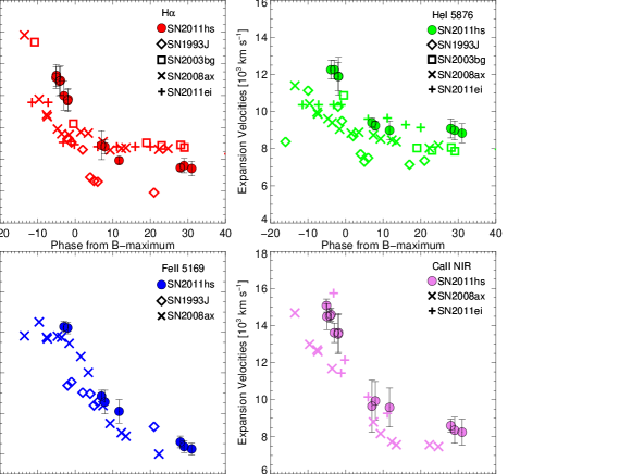
Figure 9: Expansion velocities measured from the minimum of the absorption lines of the main ions in SN 2011hs spectra. Velocities of the same ions in the spectra of the same SN sample of Figure 8. Uncertainties affecting each line velocity have been taken equal to three times the standard deviation from the minimum position average.

5.2 NIR Spectroscoopy

In Fig.10, we show the four spectra we obtained in the NIR wavelength range. They basically cover two epochs of the SN spectral evolution, pre-maximum and 1-month after maximum phase. The spectra obtained are precious, as only a few NIR spectroscopic data have been published to date of this class of SNe.
The $-2$ days spectrum is almost featureless, with exception of strong features at $\sim 1.03\mu$ m and $\sim 1.22\mu$ m. The former may be associated to He I $\lambda 1.083\mu$m with an expansion velocity of $\sim$13,800  km s^-1. Such a velocity is higher than those measured in the optical spectra taken at similar epochs, that may suggest a contamination by other ions, e.g. Mg II and/or C I. The presence of C I can be probably excluded because then we would expect other strong lines from the same ion. In general, He lines occur in spectral regions strongly affected by different metal absorptions (Lucy, 1991), with exception of the He I $\lambda 2.058\,\mu$m line, which has been claimed as the only direct evidence of the presence of this ion (Hamuy et al. 2002; Valenti et al. 2008; Modjaz et al. 2009; Stritzinger et al. 2009). For SN 2011hs, there is a clear detection of the He I line at $\lambda 2.058\,\mu$m: marginally detected at $-2$d, a strong P-Cygni emerges one month after maximum (see Fig.10).
It is possible that Pa$\gamma$ absorption contaminates the $\sim 1.03\mu$m feature in the $-2$ days spectrum, supported by the identification of the minimum at $\sim 1.22\,\mu$m as Pa$\beta$, with an expansion velocity of $\sim$13,900  km s^-1, similar to that measured for the optical H$\beta$ and H$\gamma$ at the same epoch (Fig. 9). Unfortunately, Pa$\alpha$ lies in a region where the Earth s atmosphere is opaque, so it cannot be detected.
In Fig.10, we compare SN 2011hs to SN 2008ax (Taubenberger et al., 2011) at similar epochs. For SN 2008ax, a significant contribution of the H I Paschen lines to the He I $\lambda 1.083\,\mu$m absorption feature has been excluded, because of the weakness of the Pa$\beta$ line already in the pre-maximum spectrum. At later phases, we can recognize in SN 2011hs the emergence of an emission band at $\sim 1.19\,\mu$m likely attributed to Si I $\lambda\lambda 1.198,1.203\,\mu$m blended with Mg I $\lambda 1.183\,\mu$m. The latter contributes also to the emissions at $\sim 1.50\,\mu$m and at $\sim 1.58\,\mu$m. The O I $\lambda 0.926\,\mu$m and O I $\lambda 1.315\,\mu$m are responsible for the emission bands at $\sim 0.93\mu$m and 1.31$\mu$m, respectively.

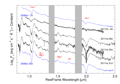
Figure 10: NIR spectra of SN 2011hs, compared with those of SN 2008ax (Taubenberger et al., 2011) in pre-maximum and one month post-maximum phases. The spectra have been corrected for redshift and reddening with the same values as adopted for the optical data. Grey bands indicate the telluric bands position.

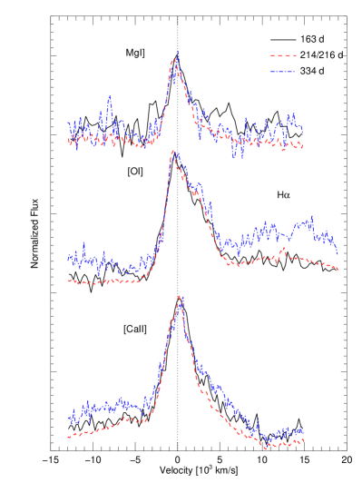
Figure 11: Nebular emission line profiles of SN 2011hs from 163 days, 214/216 days and 334 days spectra.

5.3 Nebular Spectral Line Profile

The profiles and velocities of nebular lines can provide valuable information concerning the geometry of SN explosion and the distribution of the emitting material (Fransson & Chevalier 1987, 1989; Mazzali et al. 2005; Maeda et al. 2008). Plotted in Fig. 11 are the emission line profiles, in velocity space, of the predominant ions Mg I] $\lambda$4570, [O I] $\lambda$$\lambda$6300, 6363 and [Ca II] $\lambda$$\lambda$7291,7324, from spectra taken at 163, 214, 216 and 334 days after $t(B)_{max}$ (see Tab. 7). Since no major evolution is detectable between them, the two spectra taken at +214d and +216d have been combined to improve the signal-to-noise (indicated as 214/216 days). The nebular line profiles reveal similar widths and no evidence for asymmetries, suggesting a fairly symmetric expanding ejecta. A strong box-like emission profile red-ward of the [O I] doublet line is also present and identified as H$\alpha$ emission line. Such feature has been detected in previous SE SNe, e.g. SN1993J (Patat, Chugai, & Mazzali, 1995), SN 2007Y (Stritzinger et al., 2009) and SN 2008ax (Taubenberger et al., 2011), and claimed to be the product of the interaction between a fast expanding shell of H from the SN and the dense CSM (Chevalier & Fransson, 1994). This explanation raised some inconsistencies between the shock interaction scenario and the low H$\alpha$ velocity observed in e.g. SN 2008ax (Taubenberger et al., 2011).
An alternative interpretation, given by Maurer et al. (2010), explains such late phase H$\alpha$ emission as the result of mixed and strongly clumped H and He. In this case, radioactive energy deposition can power H$\alpha$ completely without any need for an additional source of energy. Clumpiness can significantly increase the relative strength of H$\alpha$, and combined with the mass of He or H in such mixed fraction, makes possible to reproduce the spectra in several combinations (see Maurer et al. 2010). Although this prevents us from determining the H/He mass involved, it can explain the different observed shapes in late H$\alpha$ emission profiles: strong and box-shaped, like in SNe1993J , 2007Y and 2008ax; or weak emissions, like for SNe 2001ig and 2003bg (Maurer et al., 2010). Most importantly, it solves the contradictions with the X-ray observations, when the shock interaction is assumed to be responsible for the H$\alpha$ emission (see e.g. Chevalier & Soderberg 2010). In SN 2011hs the H$\alpha$ emission has a velocity of $\sim$6,000$-$8,000 km s^-1 measured at the edge of the observed feature, similar to that found by Taubenberger et al. (2011) for SN 2008ax and lower than that found for SN 2007Y (around 9,000$-$11,000  km s^-1; Stritzinger et al. 2009).
Finally, a bump blue-ward of the [Ca II] line is also visible, as previously seen in the nebular spectra of SNe 2008ax (Taubenberger et al., 2011) and 2011ei (Milisavljevic et al., 2013) and probably due to a blended emission from He I $\lambda$7065 and [Fe II] $\lambda 7155$.
Fransson & Chevalier (1987, 1989) have shown that the [Ca II]/[O I] ratio is a sensitive tracer of the core mass, giving useful insight into the main sequence progenitor mass. Staying relatively constant at late phases, the ratio decreases for more massive cores. In SN 2011hs, the strength of [Ca II] $\lambda$$\lambda$7291,7324 is comparable to that of [O I] $\lambda$$\lambda$6300, 6364, with a mean ratio $\sim$1.2 measured from the three nebular spectra. As a reference, such ratio was about 0.5 in SN 1998bw, which was found to have a progenitor with a mass $\approx$40 M_⊙ (Iwamoto et al., 1998). For SNe 2007Y and 1993J a ratio $>$0.5 was measured, suggesting a progenitor star with a main sequence mass much lower than the progenitor of SN 1998bw, i.e. $\loa$ 20 M_⊙ (Stritzinger et al. 2009; Nomoto et al. 1993; Podsiadlowski et al. 1993). For SN 2008ax, Taubenberger et al. (2011), measuring a [Ca II]/[O I] $\sim$0.9, claimed a low-mass progenitor in a binary system, rather than a single massive WR star. Thus having a line flux ratio slightly higher than that of SN 2008ax, a low-mass progenitor star can be proposed for SN 2011hs, too.

5.4 Nebular Spectrum Modelling

In order to establish the properties of the inner ejecta with higher accuracy, we have modelled the 214/216d nebular spectrum. Unfortunately due to the lack of simultaneous photometric observations (or at least close in time), the flux calibration of the 334d nebular spectrum is uncertain, thus it cannot be used for modelling. We used our non-local thermodynamic equilibrium (NLTE) code (e.g. Mazzali et al. 2007). The code computes the emission of gamma-rays and positrons from the decay of ⁵⁶Ni into ⁵⁶Co and hence ⁵⁶Fe. These are then allowed to propagate in the SN ejecta, and their deposition is followed with a MonteCarlo scheme as outlined in Cappellaro et al. (1997). Energy deposited heats the gas, which is a mixture of various elements seen in the SN ejecta, through collisional processes. Heating is balanced by cooling via line emission. The balance of these two processes is computed consistently with the occupation of the atomic energy levels, in NLTE. Emission is mostly in forbidden lines, although some permitted transitions are also effective in cooling the ejecta. Although the code is available in both a one-zone and a stratified version, here we use the one-zone approach, because we do not have a viable explosion model available for SN 2011hs. Observed and synthetic spectrum are plotted in Fig. 12. We can establish from the line profiles a typical line width of 3500 km s^-1. This matches the width of most emission features, except for H$\alpha$, which is caused by a different mechanism and is broader, reflecting the distribution of H. Interestingly, H$\alpha$ does not develop a boxy profile, possibly indicating some mixing of H down to low velocities. We find that a reasonable fit to the spectrum (shown in Fig. 12), excluding H emission and the He zone, requires a small ⁵⁶Ni mass, 0.04 M_⊙. The ejecta mass included within the boundary velocity is also quite small, 0.23 M_⊙, as expected given the rapid evolution of the SN light curve. These values are reasonably consistent with a He core of 3-4 M_⊙ found with the modeling of the bolometric light curve (cf. Sect. 6.2). The most abundant element in the inner ejecta is Oxygen, as usual, with a quite small mass of 0.13 M_⊙, consistent with a low-mass star core-collapse scenario (Limongi & Chieffi, 2003) and what we found in Sections 5.3 and 6.2. Other elements that are seen in emission are C, Mg, Ca, Fe and Na.

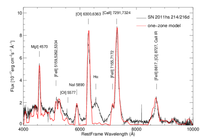
Figure 12: The nebular spectrum of SN 2011hs taken at 214/216 d compared with the synthetic spectrum.

6 SN 2011hs physical parameters

When no pre-explosion images are available, one of the most direct ways to estimate the physical parameters of a SN progenitor is by comparing the observations with the models of the light curve and the photospheric velocity evolution of the SN. The observed quantities adopted in the present work are a) the bolometric light curve (see Sect. 6.1), derived from the broad band photometry and b) the photospheric velocity measured from Fe II lines. For the models, we used a one-dimensional, Lagrangian code described in Bersten, Benvenuto, & Hamuy (2011).

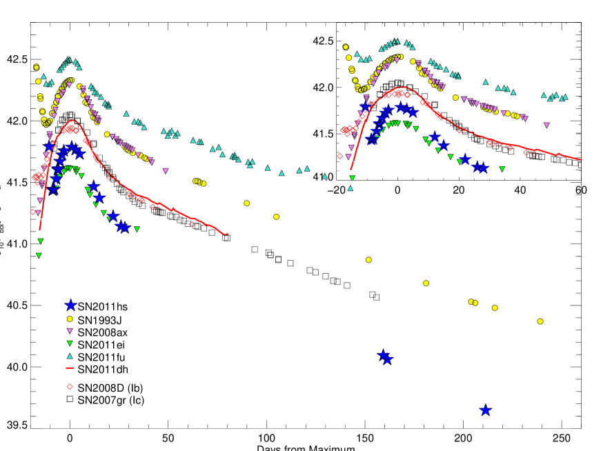
Figure 13: BVRI pseudo-bolometric light curve of SN 2011hs compared to those of the Type IIb SNe  1993J (Barbon et al. 1995; Richmond et al. 1996), 2008ax (Pastorello et al. 2008, Taubenberger et al. 2011), 2011dh (Ergon et al., 2013); 2011ei, (Milisavljevic et al., 2013) and 2011fu, (Kumar et al., 2013), and the Type Ib SN 2008D (Mazzali et al. 2008, Tanaka et al. 2009) and Type Ic SN 2007gr (Valenti et al., 2008). A zoom-in on the early photospheric evolution is given in the upper-right corner.

6.1 Bolometric Light Curve

To construct the bolometric light curve, we first corrected the magnitudes for extinction and converted them to flux densities at the effective wavelength of the corresponding bandpass. The total flux was then obtained by integrating over the UV-opt-NIR wavelength range and, next, the integrated bolometric flux was converted into luminosity using the adopted distance (Section 3). The bolometric luminosity was computed for all the epochs by keeping the $R$ band light curve as reference and extrapolating the missing data in other bands by assuming a constant colour.
We estimated the UV contribution to the bolometric emission to be around 20 per cent at very early phases and below 5% after maximum light. On the other hand, the NIR contribution did not exceed 30% before maximum, while increasing to 50% after. Since a comparison of SN 2011hs with previously studied SE SNe would require making strong assumptions on the UV and NIR contributions to the bolometric flux for those missing data at these wavelengths, in order to be conservative, we compare their pseudo-bolometric flux, obtained by integrating only the BVRI light curves. Thus, we compiled and compared the pseudo-bolometric curve of SN 2011hs with those of the Type IIb SNe  1993J (Barbon et al. 1995; Richmond et al. 1996), 2008ax ( Pastorello et al. 2008, Taubenberger et al. 2011), 2011dh (Ergon et al., 2013); 2011ei (Milisavljevic et al., 2013) and 2011fu, (Kumar et al., 2013), the Type Ib SN 2008D (Mazzali et al. 2008, Tanaka et al. 2009) and Type Ic SN 2007gr (Valenti et al., 2008). The comparison is displayed in Fig. 13. After SN 2011ei, SN 2011hs has one of the faintest bolometric luminosities at peak, with L_BVRI= 6.1$\times$10⁴¹ erg s^-1. This indicates a smaller amount of ⁵⁶Ni ejected with respect to the previous SE SNe: indicatively we can expect a total ⁵⁶Ni mass between 0.03 M${}_{\odot}<$ M${}_{Ni}<$ 0.09 M_⊙, corresponding to the masses ejected by SN 2011ei (Milisavljevic et al., 2013) and SN 2008D (Mazzali et al., 2008), respectively. The ⁵⁶Ni mass is not the only factor that determines the light curve shape; the explosion energy and the ejected mass play an important role, too. SN 2011hs has a narrower light curve than the other SE SNe. Considering Arnett’s relation (Arnett 1982, 1996) for which $\tau_{\rm peak}\propto M_{\rm ej}^{3/4}E^{-1/4}$ and assuming a similar explosion energy, such narrow light curve width points to a smaller ejected mass, and, therefore, a smaller progenitor mass.

6.2 The Light Curve modelling

To calculate models for the bolometric light curve and the photospheric velocity evolution of SN 2011hs, we used a code that solves the hydrodynamics and radiation transport in an expanding ejecta including the gamma-ray transfer in grey approximation (Bersten, Benvenuto, & Hamuy, 2011). He-core stars with different masses calculated from a single stellar evolutionary code (Nomoto & Hashimoto, 1988) are used as the initial configurations to explode (Tanaka et al., 2009). The initial density structures are artificially modified by attaching a thin H-rich layer to the He core as required for a Type IIb classification. The method used to attach the envelope to the core was recently presented in the modelling of SN 2011dh (Bersten et al., 2012). In this way it is possible to artificially modify the progenitor radius and test it against observations. As mentioned in Section 4, the light curve of a SE SN has two characteristic phases: (a) the early UV/optical emission or “cooling phase” powered by the energy deposited by the shock wave and (b) a re-brightening to a broad maximum due to the decay of radioactive material synthesized during the explosion. Before rising to the light curve maximum, a minimum or “valley” can be distinguished. While the global properties of a SN such as explosion energy ($E$), ejected mass ($M_{\mathrm{ej}}$), and the ⁵⁶Ni mass can be obtained by modelling the light curve around maximum, observations of the early emission provide unique information about the progenitor radius. In the case of SN 2011hs, there is a single data point during the cooling phase that we used to place constraints on the possible progenitor radius.
Firstly we compared the observables and the theoretical bolometric light curves and velocities focusing on the evolution around the maximum light to obtain the general properties. An important point required to reliably determine physical parameters is the knowledge of the explosion time (t_exp). Unfortunately, for SN 2011hs there is no pre-explosion information available to help us determine t_exp, i.e. non-detection images taken shortly before the explosion (see Milisavljevic et al. 2011), hence, our estimate must rely on comparisons with other Type IIb SNe. One possibility is to match the valley point of the light curve of SN 2011hs with that of SN 1993J, for which the explosion date and thus, the cooling duration is well known. In this case, in order to have an 8-day long cooling branch, t_exp should occur $\sim$6 days before the SN discovery, $\Delta$t = t${}_{\mathrm{discovery}}-$ t_exp= 6 days. On the other hand, comparing the cooling in the $R$ band, we find a declining rate for SN 2011hs ($\Delta R$=0.46 mag d^-1), which is more than twice that of SN 1993J ($\Delta R$=0.21 mag d^-1, Richmond et al. 1996), implying a 4-day long branch (similar to that of SN 2011dh) and a $\Delta$t = 2 days. The latter case implies a rise time to maximum light ($t(V)_{max}$) for SN 2011hs of $\approx$13 days, which is far from the observed typical value of $t(V)_{max}\approx$20 days (Richardson, Branch, & Baron 2006; Drout et al. 2012).

Alternatively, in order to have a $t(V)_{max}\sim$20 days after the explosion SN 2011hs should have exploded with a $\Delta$t = 9 days. Such a t_exp would imply an extremely large radius for a Type IIb SN progenitor star (Bersten et al., 2012), therefore we discard this scenario.
Thus, in the following analysis, we adopt a $\Delta t=6$ days, assuming that SN 2011hs exploded at $t_{\mathrm{exp}}=2,455,872\pm 4$ JD, with a $t_{\mathrm{valley}}\sim 8$ days and $t_{\mathrm{max},V}\sim 16$ days. This is in agreement with the explosion epoch obtained through the radio light curve modelling (see Section 7). Nevertheless, later in this section we further discuss the possibility of an earlier t_exp.

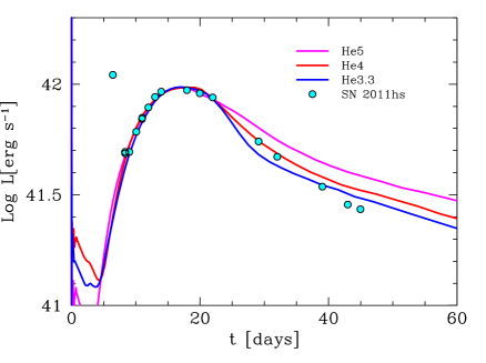
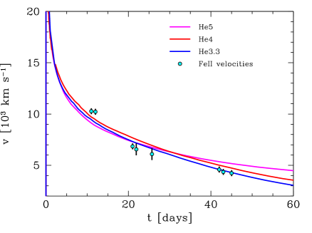
Figure 14: (Upper panel) Observed bolometric light curve of SN 2011hs (points) compared with the results of the light curve calculations for models He$3.3$ (blue line), He4 (red line) and He5 (purple line). (Lower panel) Evolution of the photospheric velocity for models He$3.3$ ( blue line), He4 (red line) and He5 (purple line) compared with measured Fe II line velocities of SN 2011hs.

We have calculated a set of models with different values of $E$, He-core mass and mixing of ⁵⁶Ni to try to reproduce the bolometric light curve around the main peak along with the photospheric velocity evolution. Specifically, we use three different pre-SN models with He cores of $3.3$ $M_{\odot}$ (He$3.3$), 4 $M_{\odot}$ (He4) and 5 $M_{\odot}$ (He5), which correspond to the stellar evolution of single stars with main-sequence masses of 12 $M_{\odot}$, 15 $M_{\odot}$ and 18 $M_{\odot}$, respectively. Fig. 14 shows the best results of such models (He$3.3$ in blue, He4 in red and He5 in purple solid lines) for the bolometric light curve (upper panel) and for the photospheric velocities (lower panel) compared with the observations. Assuming $M_{\mathrm{ej}}$= $M_{\mathrm{total}}-M_{\mathrm{cut}}$ (where $M_{\mathrm{cut}}$ is the mass of the compact remnant assumed to be $1.5$ $M_{\odot}$), the parameters used in each calculation are (a) for He$3.3$: $E=8\times 10^{50}$ erg, $M_{\mathrm{ej}}=1.8$ $M_{\odot}$ and a ⁵⁶Ni mass of $0.037$ $M_{\odot}$; (b) for He4: $E=9\times 10^{50}$ erg, $M_{\mathrm{ej}}=2.5$ $M_{\odot}$ and ⁵⁶Ni mass of $0.038$ $M_{\odot}$; and (c) for He5: $E=1\times 10^{51}$ erg, $M_{\mathrm{ej}}=3.5$ $M_{\odot}$ and ⁵⁶Ni mass of $0.040$ $M_{\odot}$. In all cases the degree of ⁵⁶Ni mixing assumed was $\approx$ 80% of the initial mass. From Fig. 14, we see that He$3.3$ and He4 models give a reasonably good match to the observations, while He5 model, which can also reproduce the light curve for $t<$ 20 days, clearly fails at later epochs. Since changing the physical parameters for such initial mass does not improve the agreement with the observed data, we discarded models with He core mass $\geq$5 $M_{\odot}$. The models He$3.3$ and He4 can be considered at the same level of agreement with the data.

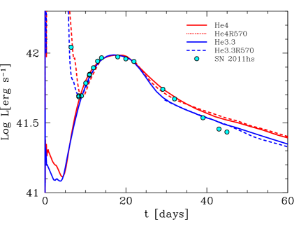
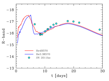
Figure 15: (Upper panel) Observed bolometric light curve of SN 2011hs (points) compared with the results of the light curve calculations for models He$3.3$ (blue line) and He4 (red line). Two models with larger progenitor radii, He$3.3$R570 (blue dot line), He4R570 (red dot line), are also shown (see text for details). Only with extended structures of $R>500R_{\odot}$ it is possible to reproduce the earliest data point and the light curve valley. (Lower panel) $R$-band light curve for extended models He3R570 (blue line), He4R70 (red line) compared with the observations.

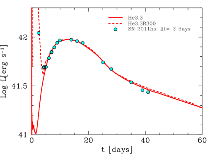
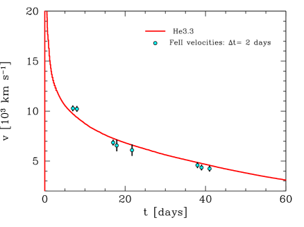
Figure 16: (Upper panel) Observed bolometric light curve of SN 2011hs assuming the explosion occured two days before the SN discovery ($\Delta t=2$; cyan points) compared with the results of the light curve calculations for the He$3.3$ model with (dashed line) and without (solid line) an attached H-rich envelope. (Lower panel) Evolution of the photospheric velocity for models He$3.3$ compared with measured line velocities of Fe II.

Both models, He3.3 and He4, have a compact structure with a radius $\approx$2 R_⊙ and clearly cannot reproduce the earliest data point as well as the luminosity of the valley observed in SN 2011hs. To improve the fit during the cooling phase, we have attached several envelopes to He3.3 and He4 with different radii. The best models we found were a model with a radius of 570 R_⊙ attached to He3.3 (He3.3R570) and to He4 (He4R570). The mass of the envelope we assumed for both models was $M_{\mathrm{env}}<0.5M_{\odot}$. Models are shown in Fig. 15 (upper panel). Since we have no information on the colour evolution of SN 2011hs along the cooling decline, we could introduce an uncertainty in the bolometric flux estimation with the adopted assumption of constant color (see Sect. 6.1). Thus, we also compare SN 2011hs $R$ band light curve with the same models found using the bolometric one. Fig. 15 (lower panel) confirms the good agreement of the models (especially for the He4 model) with the observations. However, we stress that in order to calculate the theoretical $R$ band light curve, we assumed a black body emission which may not necessarily be the case, especially at late epochs.
Given the uncertainties affecting the observional data (extinction, t_exp, etc) and the models (simple prescription of the radiation transfer, one dimensional calculations, differences in the initial model from different stellar evolutionary calculation, etc), the models indicate a range of validity for the physical parameters of SN 2011hs rather than robust estimations. Our analysis suggests a progenitor star composed of a He core of 3–4 $M_{\odot}$ and a thin H-rich envelope of $<0.5M_{\odot}$, for a main sequence mass estimated to be in the range of 12–15 $M_{\odot}$ (based on our stellar initial model). To reproduce the early light curve of SN 2011hs, a progenitor radius in the range of 500–600 R_⊙ is required. An explosion energy of $E\sim 8.5\times 10^{50}$ erg, a ⁵⁶Ni mass of about 0.04 M_⊙ and a mixing of 80 $\%$ of the initial mass reproduce well the observations around the light curve maximum. Finally, note that our modelling rules out progenitors with He core mass $>5M_{\odot}$, which excludes main sequence masses above $20$ $M_{\odot}$. For comparison, in the case of SN 2011dh initial masses above 25 $M_{\odot}$ were ruled out (Bersten et al. 2012), thus this possibly implies that the progenitor of SN 2011hs was less massive than that of SN 2011dh.

Short rise time

We analyze the possibility of $\Delta t=2$ days, although this value would imply a rise time to the peak for SN 2011hs of $\approx$13 days, which is lower than the typical values for SE SNe and in disagreement with the result of radio data modeling. We have tested the same initial models as in the previous section, i.e. He core masses of $3.3$ M_⊙ (He$3.3$), 4 M_⊙ (He4) and 5 M_⊙ (He5). For models He4 and He5, we could not find a set of parameters that can reproduce simultaneously the light curve and the photospheric velocities. However, for the least massive model, He$3.3$, we found a very good agreement with the observations. Fig. 16 shows this model with and without an attached envelope, compared with the observations. The physical parameters used in this simulation are $E=6\times 10^{50}$ erg, ⁵⁶Ni mass of 0.037 $M_{\odot}$, an H-rich envelope with a radius of $\approx$ 300 $R_{\odot}$ and a mass of $0.1$ M_⊙ (He$3.3$R300). However, we had to assume almost complete mixing of ⁵⁶Ni ($\approx$ 98% of the initial mass) to fit the rising part of the light curve. Note that the ⁵⁶Ni mass is the same as that found in the previous section, but in this case a less energetic explosion and a less extended progenitor were needed. This analysis shows that the two parameters that change most dramatically with the assumed explosion time are the mixing and the progenitor radius. Therefore, it is important to know $t_{\mathrm{exp}}$ as best as possible if one wants to predict these parameters accurately. We believe that there is no reason to assume such extreme ⁵⁶Ni mixing as there is no strong evidence of large asymmetries in the explosion of SN 2011hs. Therefore we consider this fast rise-time scenario as less likely than the one presented previously. However, note that even with this $t_{\mathrm{exp}}$ we had to assume an extended object (300 $R_{\odot}$) to reproduce the earliest data point.

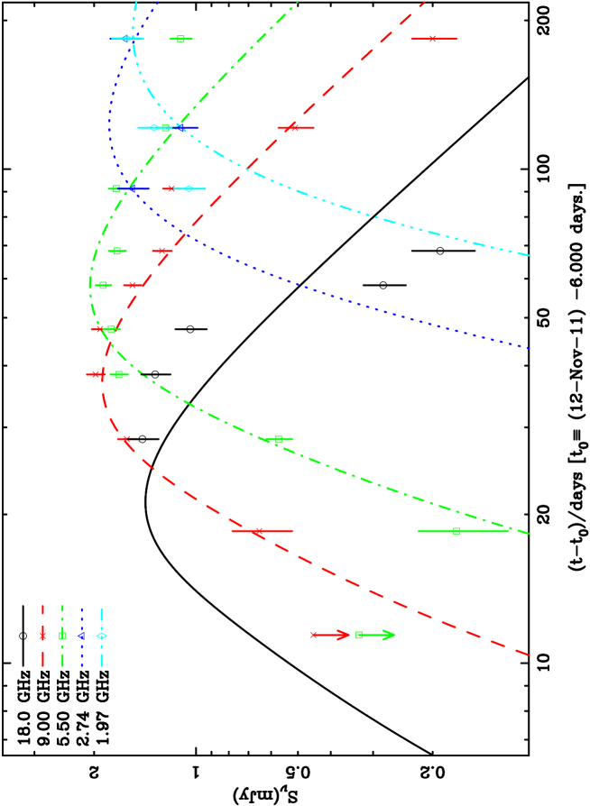
Figure 17: Radio light curves of SN 2011hs at frequencies of 18.0 GHz (black circles, solid line), 9.0 GHz (red crosses, dashed line), 5.5 GHz (green squares, dash-dotted line), 2.7 GHz (blue triangles, dotted line), and 2.0 GHz (cyan diamonds, dash-triple dotted line). The curves are a model fit to the data, as described in the text.

7 Radio data analysis

Radio studies of SNe (RSNe) can provide valuable information about the density structure of the circumstellar medium, the late stages of stellar mass-loss, and clues to the nature of the progenitor object (Weiler et al., 2002). Radio emission has only been detected from core-collapse SNe, and observed among these to date only from 12 Type IIb SNe: SN 1993J (Weiler et al., 2007), SN 1996cb (Weiler et al., 1998), SN 2001gd (Stockdale et al., 2007), SN 2001ig (Ryder et al., 2004), SN 2003bg (Soderberg et al., 2006), SN 2008ax (Stockdale et al., 2008a; Roming et al., 2009), SN 2008bo (Stockdale et al., 2008b), SN 2010P (Herrero-Illana et al. 2012; Romero-Cañizales et al. 2013), SN 2011dh (Horesh et al., 2012; Krauss et al., 2012; Soderberg et al., 2012), SN 2011hs (Ryder et al., 2011), PTF 12os (Stockdale et al., 2012) and the recent SN 2013ak (Chakraborti et al., 2013).
It has been found that the radio “light curve” of a core-collapse supernova can be broadly divided into three phases. First, there is a rapid turn-on with a steep spectral index ($\alpha>2$, so the SN is brightest at higher frequencies) due to a decrease in the line-of-sight absorption. After some weeks or months have elapsed, the flux reaches a peak, turning over first at the highest frequencies. Eventually, the SN begins to fade steadily, and at the same rate at all frequencies, in the optically-thin phase.

Figure 18: Evolution of spectral index $\alpha$ for SN 2011hs, plotted linearly as a function of time, between 5.5 and 9.0 GHz. The curve is a model fit to the data, as described in the text.

The ATCA radio light curve of SN 2011hs is plotted in Figure 17, while the time evolution of the spectral index $\alpha$ (where flux $S\propto\nu^{+\alpha}$) between simultaneous positive detections at 5.5 and 9.0 GHz is plotted in Fig. 18.
As can be seen in Fig. 17, the radio light curves for SN 2011hs are broadly consistent with the typical scenario described above. The emission had already peaked at 18 GHz prior to the first observation at that frequency; the peak at 9 GHz occurred about a month after discovery; the peak at 5.5 GHz almost a month later; and the SN may just have peaked at 2 GHz by the time observations ended. There are a few points at each frequency which appear to exhibit significant departures from a smooth evolution, but none are as achromatic or periodic as that displayed by SN 2001ig or SN 2003bg. On the other hand SN 2011hs never rose above a flux of 2 mJy at any frequency, which was about where monitoring of SN 2001ig had to be suspended with the much less sensitive ATCA$+2\times 128$ MHz bandwidths.

The general properties of supernova radio light curves as outlined above are quite well represented by a modified version of the “minishell” model of Chevalier (1982), and have been successfully parameterised for more than a dozen RSNe (see Table 2 of Weiler et al. 2002). Radio synchrotron emission is produced when the SN shock wave ploughs into an unusually dense circumstellar medium (CSM). Following the notation of Weiler et al. (2002) and Sramek & Weiler (2003), we model the multi-frequency evolution as:

$$S{\rm(mJy)}=K_{1}{\left({\nu}\over{\rm 5~{}GHz}\right)^{\alpha}}{\left({t-t_{0}}\over{\rm 1~{}day}\right)^{\beta}}e^{-{\tau_{\rm external}}}$$

$$\times{\left({1-e^{-{\tau_{\rm CSM_{clumps}}}}\over{\tau_{\rm CSM_{clumps}}}}\right)}{\left({1-e^{-{\tau_{\rm internal}}}}\over{\tau_{\rm internal}}\right)}$$ (1)

with

$$\tau_{\rm external}=\tau_{\rm CSM_{homog}}+\tau_{\rm distant}$$ (2)

where

$$\tau_{\rm CSM_{homog}}=K_{2}{\left({\nu}\over{\rm 5~{}GHz}\right)^{-2.1}}{\left({t-t_{0}}\over{\rm 1~{}day}\right)^{\delta}},$$ (3)

$$\tau_{\rm distant}=K_{4}{\left({\nu}\over{\rm 5~{}GHz}\right)^{-2.1}},$$ (4)

and

$$\tau_{\rm CSM_{clumps}}=K_{3}{\left({\nu}\over{\rm 5~{}GHz}\right)^{-2.1}}{\left({t-t_{0}}\over{\rm 1~{}day}\right)^{\delta^{\prime}}},$$ (5)

with the various $K$ terms representing the flux density ($K_{1}$), the attenuation by a homogeneous absorbing medium ($K_{2}$, $K_{4}$), and by a clumpy/filamentary medium ($K_{3}$), at a frequency of 5 GHz one day after the explosion date $t_{0}$. The $\tau_{\rm CSM_{homog}}$ and $\tau_{\rm CSM_{clumps}}$ absorption arises in the circumstellar medium external to the blast wave, while $\tau_{\rm distant}$ is a time-independent absorption produced by e.g., a foreground H ii region or more distant parts of the CSM unaffected by the shock wave. The spectral index is $\alpha$, $\beta$ gives the rate of decline in the optically-thin phase; and $\delta$ and $\delta^{\prime}$ describe the time dependence of the optical depths in the local homogeneous, and clumpy/filamentary CSM, respectively (see Weiler et al. (2002) and Sramek & Weiler (2003) for a detailed account of how these parameters are related). For lack of sufficient high-frequency data prior to the turnover to constrain it, we adopt ${\tau_{\rm internal}}=0$.

In order to assess the gross properties of SN 2011hs, we have fit this standard model to all the data points plus upper limits in Table 8. The actual date of explosion $t_{0}$ is found to be at least 5 days prior to discovery in agreement with the hydrodynamical modeling results (see Sect.6.2); slightly better fits are possible for later dates, but only if the value of $\alpha$ approaches non-physical values. The full set of model parameters which yields the minimum reduced $\chi^{2}$ is given in Table 10, and the model curves are plotted in Fig. 17. For comparison, we show in Table 10 the equivalent parameters for three other well-sampled Type IIb RSNe that were fitted using the parametrization we used here: SN 2001ig (Ryder et al., 2004) in NGC 74724, SN 1993J (Weiler et al., 2007) in M81, and SN 2001gd (Stockdale et al., 2003) in NGC 5033. Fixing the value of $\delta$ to be $(\alpha-\beta-3)$, as in the Chevalier (1982) model for expansion into a CSM with density decreasing as $r^{-2}$, also resulted in a slightly better fit overall but a much steeper rise to maximum that misses the earliest data at 5.5 and 9.0 GHz.

Both the optically-thin spectral index $\alpha$, and the rate of decline $\beta$ are much steeper in SN 2011hs than in any of the other Type IIb SNe, and the time to reach peak flux at 5 GHz is also much shorter.
Using the methodology outlined in Weiler et al. (2002) and Sramek & Weiler (2003), we can derive an estimate of the progenitor’s mass-loss rate, based on its radio absorption properties. Substituting our model fit results above into their equations 11 and 13 we find that

$$\frac{\rm\dot{M}/(M_{\odot}\ {\rm yr}^{-1})}{w/{\rm(10\,km\ s^{-1})}}=(2.0\pm 0.6)\times 10^{-5}$$

where $w$ is the mass-loss wind velocity, and the ejecta velocity measured from the optical spectra (Fig. 7) is in the range $8,000-12,000$ km s^-1. The deceleration parameter $m$ is given by $m=-\delta/3$ (equation 6 of Weiler et al. 2002) leading to $R\propto t^{0.44}$ which is consistent with the rapid deceleration in expansion velocity seen in Fig.  9. Despite similar light curve fitting parameters, the derived mass-loss rates for the progenitors of SN 2011hs and SN 1993J are rather different, while those of SN 2001ig, and SN 2001gd are all remarkably similar (see Table. 10). In many respects SN 2011hs has behaved more like a Type Ib/c SN than most “normal” Type II SNe. The peak luminosity at 5 GHz was similar to that attained by SN 1993J, but only half as much as SN 2001ig or SN 2001gd. Recently, assuming the synchrotron self absorption (SSA) as the dominant absorption mechanism, Chevalier & Soderberg (2010) estimated the radio shell velocity at the time of the peak radio luminosity (as in Chevalier 1998) for a sample of SE SNe, and found that some of the Type IIb SNe show rapid radio evolutions for a given luminosity, indicating high shell velocities (e.g. around 30,000$-$50,000 km s^-1) similar to Type Ib/c SNe. Based on this, they propose dividing Type IIb SNe in the (L_peak vs $t_{peak}$) plane (see their Fig.1, here adapted in Fig. 19) into two groups, eIIb and cIIb SNe, with Type eIIb SNe (like SNe 1993J and 2001gd) having more extended progenitor, a denser wind and a slower shock velocity, than those of Type cIIb (e.g. SNe 2008ax, 2003bg and 2001ig), supposed to come from a more compact progenitor star.
Nevertheless, SN 2011dh was found to have compact radio properties (Soderberg et al., 2012), while, as already discussed, there are strong evidences for an extended progenitor star (YSG; Bersten et al. 2012; Ergon et al. 2013; Van Dyk et al. 2013). Note that the position of SN  2001gd changes if, instead of Stockdale et al. (2003), we adopt the results from Stockdale et al. (2007), where a contribution from the SSA mechanism in the modeling of the data was included. This assumption moves the position of SN 2001gd close to SN 2001ig, in the eIIb SNe “region”, making the separation even less definitive. Similarly, SN 2011hs seems to do not follow the proposed Type eIIb/cIIb separation: indeed, its position in the (L_peak vs $t_{peak}$) plot is close to that of SN 2011dh in the compact velocity contour, while the modeling of the optical emission here presented, points to an extended progenitor.
These findings seem to suggest that the radio emission is not a good indicator of the progenitor size, although a larger sample of Type IIb SNe observed at these wavelengths is needed to reach a firmer conclusion.

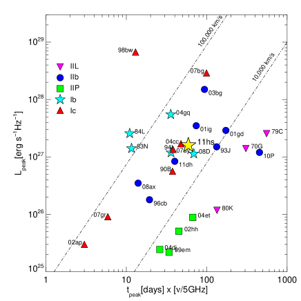
Figure 19: Peak spectral radio luminosity at 5 GHz plotted versus the time of the peak at the same frequency measured for supernovae of Types Ib/c, IIb and IIL/P. The observed supernovae are designated by the last two digits of the year and letters. The references for the peak values used in this plot are in Romero-Cañizales et al. (2013), where the radio observations towards SN 2010P are also presented. Point-dashed lines show the mean velocity of the radio shell, with the assumption of the SSA as responsible for the flux peak (for details see Chevalier 1998).

8 Conclusions

We have presented detailed spectrophotometric observations of SN 2011hs taken from a few days after the explosion up to the nebular phase. The reported follow-up collects data from the X-ray to radio wavelengths, turning this object into one of the most comprehensively studied Type IIb SNe.
We found that SN 2011hs was a relatively faint (M_B = -15.6 mag) and red Type IIb SN, characterized by a narrow light curve shape, indicating a rapid evolution. Its spectral evolution showed the metamorphosis typical of this class of SN, from spectra dominated by H I lines to spectra where He I features dominate. The spectra are characterized by relatively broad absorption profiles from which we measured high expansion velocities, similar to those of the fast expanding SN 2003bg. This points to a high explosion energy per unit mass, although the narrowness of the light curve and the faintness of the peak luminosity exclude the possibility of a hypernova explosion. The light curve shape could suggest a low mass progenitor star, or more specifically a low ejecta density. This could also explain the rapid evolution observed for the H I expansion velocity, with the outer region in which the H lines form, receding faster than in previously studied SNe, probably because of a lower density.
Modelling the light curve of SN 2011hs and its velocity evolution with hydrodynamical calculations, we estimated that the SN is consistent with the explosion of a 3–4 M_⊙ He-core star, from a main sequence mass of 12–15 M_⊙, ejecting a ⁵⁶Ni mass equal to 0.04 M_⊙ and characterized by an explosion energy of $E\approx 8.5\times 10^{50}$ erg. Such a scenario is also fully consistent with the results found by modeling the nebular spectrum taken at $\sim$215 days from maximum. Based on different considerations on the light curve evolution, we assumed that the explosion epoch occurred 6 days before the discovery (2,455,872 $\pm$ 4 JD). Such an explosion epoch, supported by the modelling of the radio light curve (from which we found an explosion occurred at $\ga$5 days before the discovery), assumes an adiabatic cooling phase lasting 8 days, similar to that of SN 1993J. Since the duration and the decreasing rate of the cooling branch depends mainly on the progenitor size, we could infer from it a progenitor radius of $\approx$500–600 $R_{\odot}$.
We also analyze the possibility of a short rise time (with a 4-day long cooling phase), giving an explosion scenario with the same He core mass (He3.3), slightly lower energy ($E=6\times 10^{50}$ erg) and the same ⁵⁶Ni mass ejected ($\sim$0.04 $M_{\odot}$). In contrast to the longer rise time models, we needed an extreme mixing (98%) and a smaller radius ($\approx$ 300 $R_{\odot}$ ). Although this case indicates the importance of an accurate estimation of the explosion time, the results point again to a supergiant progenitor for SN 2011hs. Finally, our modelling rules out pre-explosion stars with He core mass $>5M_{\odot}$, which implies excluding main sequence masses above $20$ $M_{\odot}$. Such a lower limit for the progenitor mass could indicate the possibility of a binary origin, although the radio light curve does not show strong deviations [as previously observed in e.g. SN 2001ig (Ryder et al., 2004) or SN 2003bg (Soderberg et al., 2006)] as a signature of the presence of a companion star. In summary, despite the fact that uncertainties in both the observational data (extinction, t_exp, bolometric corrections for the early amateurs’ points) and the modelling prevent us from reaching definitive conclusions, it stands out clearly that the SN 2011hs progenitor was a supergiant star with ZAMS mass $<$20 M_⊙, as found for SN 1993J, and most recently, for SN 2011dh.

Table 1: UVOT UV Observed Magnitudes of SN 2011hs.

UT	JD	w1	w2	m2
yyyy/mm/dd	+2,400,000	mag	mag	mag
2011 Nov 15	55880.77	18.24 (0.10)	19.07 (0.15)	19.32 (0.26)
2011 Nov 15	55881.17	18.18 (0.09)	19.09 (0.14)	$\cdots$
2011 Nov 18	55883.33	18.33 (0.10)	19.01 (0.14)	19.31 (0.19)
2011 Nov 20	55885.75	18.55 (0.12)	19.29 (0.17)	19.80 (0.29)
2011 Nov 22	55887.59	18.68 (0.15)	19.44 (0.25)	19.51 (0.30)
2011 Nov 23	55889.39	18.93 (0.15)	19.49 (0.19)	19.71 (0.29)
2011 Nov 26	55891.60	19.08 (0.17)	19.50 (0.19)	19.72 (0.27)

Table 2: UBVRI photometric sequence in SN 2011hs field as in Fig. 1.

Star ID	R.A.	Dec.	U	B	V	R	I
	h:m:s	∘:′:′′	mag	mag	mag	mag	mag
1	22:57:21.390	-43:21:59.51	15.460 (0.022)	15.039(0.012)	14.188(0.025)	13.715(0.030)	13.290(0.025)
2	22:57:22.294	-43:23:16.01	$\cdots$	15.928(0.018)	14.549(0.024)	13.677(0.034)	12.916(0.016)
3	22:57:25.878	-43:21:14.95	$\cdots$	18.449(0.032)	17.935(0.033)	17.592(0.018)	17.216(0.059)
4	22:57:22.824	-43:26:23.77	$\cdots$	17.236(0.029)	16.804(0.020)	16.532(0.032)	16.229(0.020)
5	22:57:23.152	-43:27:11.07	$\cdots$	17.289(0.062)	16.521(0.030)	16.067(0.036)	15.637(0.019)
6	22:57:06.581	-43:27:18.94	$\cdots$	15.832(0.026)	14.985(0.030)	14.518(0.037)	14.119(0.019)
7	22:56:57.117	-43:27:41.50	$\cdots$	16.047(0.028)	15.038(0.036)	14.431(0.032)	13.910(0.016)
8	22:57:05.222	-43:26:03.28	$\cdots$	19.514(0.062)	18.338(0.061)	17.583(0.040)	16.939(0.031)
9	22:56:58.012	-43:26:04.85	$\cdots$	18.738(0.020)	18.119(0.040)	17.732(0.049)	17.326(0.054)
10	22:56:48.801	-43:26:06.01	$\cdots$	17.657(0.081)	17.077(0.033)	16.711(0.049)	16.357(0.030)
11	22:56:50.025	-43:24:37.72	$\cdots$	17.930(0.066)	17.198(0.034)	16.797(0.036)	16.386(0.027)
12	22:56:57.970	-43:24:18.20	$\cdots$	17.941(0.035)	17.468(0.042)	17.156(0.039)	16.837(0.023)
13	22:56:58.428	-43:22:57.74	$\cdots$	17.868(0.071)	16.753(0.025)	16.076(0.043)	15.522(0.026)
14	22:56:50.207	-43:21:21.37	$\cdots$	19.200(0.087)	18.049(0.058)	17.391(0.040)	16.694(0.020)
15	22:57:34.719	-43:19:12.85	$\cdots$	15.953(0.055)	15.415(0.023)	15.078(0.028)	14.729(0.026)

Table 3: u^′g^′r^′i^′z^′ photometric sequence in SN 2011hs field as in Fig. 1.

Star ID	R.A.	Dec.	u′	g′	r′	i′	z′
	h:m:s	∘:′:′′	mag	mag	mag	mag	mag
1	22:57:21.390	-43:21:59.51	16.359 (0.016)	14.570 (0.017)	13.951 (0.029)	13.731 (0.025)	13.613 (0.045)
2	22:57:22.294	-43:23:16.01	18.063 (0.042)	15.253 (0.014)	13.989 (0.032)	13.410 (0.025)	13.119 (0.034)
3	22:57:25.878	-43:21:14.95	$\cdots$	18.121 (0.032)	17.789 (0.021)	17.641 (0.033)	17.582 (0.079)
4	22:57:22.824	-43:26:23.77	17.779 (0.029)	16.963 (0.012)	16.712 (0.035)	16.633 (0.022)	16.574 (0.048)
5	22:57:23.152	-43:27:11.07	18.380 (0.104)	16.853 (0.021)	16.275 (0.026)	16.068 (0.022)	15.949 (0.030)
6	22:57:06.581	-43:27:18.94	17.264 (0.016)	15.355 (0.018)	14.733 (0.028)	14.555 (0.024)	14.477 (0.031)
7	22:56:57.117	-43:27:41.50	17.760 (0.019)	15.505 (0.010)	14.659 (0.031)	14.355 (0.023)	14.221 (0.046)
8	22:57:05.222	-43:26:03.28	16.351 (0.010)	18.903 (0.020)	17.864 (0.042)	17.408 (0.065)	17.145 (0.015)
9	22:56:58.012	-43:26:04.85	19.817 (0.224)	18.352 (0.018)	17.946 (0.037)	17.757 (0.044)	17.678 (0.037)
10	22:56:48.801	-43:26:06.01	18.332 (0.022)	17.303 (0.014)	16.905 (0.036)	16.787 (0.027)	16.714 (0.053)
11	22:56:50.025	-43:24:37.72	18.866 (0.034)	17.495 (0.018)	16.994 (0.034)	16.811 (0.035)	16.720 (0.056)
12	22:56:57.970	-43:24:18.20	18.465 (0.025)	17.671 (0.015)	17.364 (0.031)	17.245 (0.042)	17.190 (0.026)
13	22:56:58.428	-43:22:57.74	19.932 (0.017)	17.280 (0.011)	16.334 (0.035)	15.981 (0.035)	15.798 (0.043)
14	22:57:34.719	-43:19:12.85	$\cdots$	$\cdots$	$\cdots$	$\cdots$	$\cdots$
15	22:56:50.207	-43:21:21.37	16.664 (0.018)	15.597 (0.013)	15.227 (0.029)	15.095 (0.02)7	15.088 (0.081)

Table 4: UBVRI Observed Magnitudes of SN 2011hs.

UT	JD	U	B	V	R	I	Instrument
yyyy/mm/dd	+2,400,000	mag	mag	mag	mag	mag
2011 Nov 12	55878.00	$\cdots$	$\cdots$	$\cdots$	15.53 (0.08)	$\cdots$	BOSS
2011 Nov 14	55879.90	$\cdots$	$\cdots$	$\cdots$	16.40 (0.07)	$\cdots$	BOSS
2011 Nov 14	55879.92	$\cdots$	$\cdots$	$\cdots$	16.42 (0.06)	$\cdots$	BOSS
2011 Nov 15	55880.57	$\cdots$	17.44 (0.02)	16.78 (0.01)	16.40 (0.01)	16.12 (0.01)	PROMPT
2011 Nov 15	55880.77	17.01 (0.07)	17.40 (0.07)	16.85 (0.08)	$\cdots$	$\cdots$	UVOT
2011 Nov 15	55881.17	16.98 (0.07)	17.29 (0.06)	16.63 (0.07)	$\cdots$	$\cdots$	UVOT
2011 Nov 16	55881.64	$\cdots$	17.27 (0.02)	16.55 (0.01)	16.14 (0.01)	15.93 (0.01)	PROMPT
2011 Nov 17	55882.53	$\cdots$	17.12 (0.02)	16.34 (0.01)	15.96 (0.01)	15.73 (0.01)	PROMPT
2011 Nov 17	55882.58	17.02 (0.03)	17.01 (0.02)	16.39 (0.02)	15.95 (0.02)	15.72 (0.02)	EFOSC2
2011 Nov 18	55883.33	17.15 (0.08)	16.94 (0.06)	16.25 (0.06)	$\cdots$	$\cdots$	UVOT
2011 Nov 18	55883.53	$\cdots$	16.98 (0.02)	16.18 (0.01)	15.76 (0.01)	15.54 (0.01)	PROMPT
2011 Nov 18	55883.54	$\cdots$	16.97 (0.01)	16.18 (0.01)	$\cdots$	$\cdots$	CATA500
2011 Nov 19	55884.57	$\cdots$	16.96 (0.05)	16.02 (0.03)	15.58 (0.01)	15.37 (0.01)	PROMPT
2011 Nov 20	55885.53	$\cdots$	16.97 (0.01)	15.92 (0.01)	15.48 (0.01)	15.23 (0.01)	PROMPT
2011 Nov 20	55885.75	17.34 (0.08)	16.86 (0.06)	15.91 (0.06)	$\cdots$	$\cdots$	UVOT
2011 Nov 22	55887.54	$\cdots$	17.02 (0.01)	15.80 (0.01)	$\cdots$	$\cdots$	PROMPT
2011 Nov 22	55887.59	17.67 (0.14)	17.03 (0.08)	15.83 (0.07)	$\cdots$	$\cdots$	UVOT
2011 Nov 23	55889.35	18.12 (0.13)	17.19 (0.06)	$\cdots$	$\cdots$	$\cdots$	UVOT
2011 Nov 24	55889.53	$\cdots$	$\cdots$	15.80 (0.01)	15.26 (0.01)	$\cdots$	PROMPT
2011 Nov 26	55891.53	$\cdots$	$\cdots$	15.88 (0.01)	15.30 (0.01)	$\cdots$	PROMPT
2011 Nov 26	55891.60	18.51 (0.16)	17.37 (0.07)	$\cdots$	$\cdots$	$\cdots$	UVOT
2011 Nov 28	55893.53	$\cdots$	17.54 (0.02)	16.02 (0.01)	15.39 (0.01)	15.01 (0.01)	PROMPT
2011 Nov 30	55895.58	$\cdots$	17.80 (0.01)	16.16 (0.01)	$\cdots$	$\cdots$	CATA500
2011 Dec 03	55898.58	$\cdots$	18.19 (0.02)	16.52 (0.01)	$\cdots$	$\cdots$	CATA500
2011 Dec 05	55900.68	$\cdots$	$\cdots$	16.79 (0.01)	15.99 (0.01)	15.55 (0.01)	PROMPT
2011 Dec 06	55901.53	$\cdots$	18.44 (0.02)	16.84 (0.01)	$\cdots$	$\cdots$	CATA500
2011 Dec 08	55903.54	$\cdots$	18.63 (0.03)	17.03 (0.01)	$\cdots$	$\cdots$	CATA500
2011 Dec 08	55903.58	$\cdots$	$\cdots$	17.05 (0.01)	16.27 (0.01)	$\cdots$	PROMPT
2011 Dec 09	55904.54	$\cdots$	18.75 (0.04)	17.14 (0.01)	$\cdots$	$\cdots$	CATA500
2011 Dec 10	55905.54	$\cdots$	18.82 (0.04)	17.17 (0.02)	$\cdots$	$\cdots$	CATA500
2011 Dec 11	55906.62	$\cdots$	$\cdots$	17.23 (0.03)	$\cdots$	$\cdots$	CATA500
2011 Dec 13	55908.54	$\cdots$	18.90 (0.04)	17.34 (0.02)	$\cdots$	$\cdots$	CATA500
2011 Dec 15	55910.54	$\cdots$	19.01 (0.03)	17.39 (0.01)	$\cdots$	$\cdots$	CATA500
2011 Dec 15	55910.60	$\cdots$	18.88 (0.04)	17.45 (0.02)	16.67 (0.02)	16.07 (0.01)	PROMPT
2011 Dec 16	55911.56	$\cdots$	18.83 (0.04)	17.48 (0.02)	$\cdots$	$\cdots$	CATA500
2011 Dec 19	55914.56	20.16 (0.06)	19.03 (0.06)	17.64 (0.06)	16.84 (0.09)	16.34 (0.10)	EFOSC2
2011 Dec 21	55916.54	20.07 (0.05)	19.06 (0.02)	17.70 (0.02)	16.88 (0.05)	16.41 (0.03)	EFOSC2
2011 Dec 21	55916.54	$\cdots$	19.03 (0.05)	17.63 (0.05)	$\cdots$	$\cdots$	CATA500
2011 Dec 26	55921.55	$\cdots$	19.14 (0.06)	17.77 (0.02)	$\cdots$	$\cdots$	CATA500
2012 Apr 30	56047.89	$\cdots$	20.93 (0.07)	20.36 (0.11)	19.67 (0.08)	19.22 (0.12)	WFCCD
2012 May 02	56049.89	$\cdots$	21.04 (0.11)	20.41 (0.06)	19.77 (0.07)	$\cdots$	WFCCD
2012 Jun 20	56099.90	$\cdots$	21.98 (0.09)	21.56 (0.13)	20.77 (0.06)	20.33 (0.05)	FORS2

Table 5: u^′g^′r^′i^′z^′ Observed Magnitudes of SN 2011hs.

UT	JD	u′	g′	r′	i′	z′	Instrument
yyyy/mm/dd	+2,400,000	mag	mag	mag	mag	mag
2011 Nov 15	55880.56	$\cdots$	17.11 (0.02)	16.58 (0.02)	16.54 (0.02)	16.50 (0.02)	PROMPT
2011 Nov 16	55881.66	$\cdots$	16.90 (0.02)	16.35 (0.02)	16.31 (0.02)	16.30 (0.02)	PROMPT
2011 Nov 17	55882.55	$\cdots$	16.70 (0.02)	16.14 (0.01)	16.12 (0.02)	16.04 (0.02)	PROMPT
2011 Nov 17	55883.56	17.78 (0.04)	16.53 (0.01)	15.95 (0.01)	15.92 (0.02)	$\cdots$	CATA500
2011 Nov 18	55883.59	$\cdots$	$\cdots$	15.95 (0.02)	15.92 (0.02)	15.87 (0.02)	PROMPT
2011 Nov 19	55884.64	$\cdots$	$\cdots$	15.79 (0.01)	15.79 (0.02)	15.70 (0.02)	PROMPT
2011 Nov 20	55885.54	$\cdots$	16.41 (0.01)	15.67 (0.01)	15.63 (0.02)	$\cdots$	PROMPT
2011 Nov 21	55886.53	$\cdots$	16.35 (0.01)	$\cdots$	$\cdots$	$\cdots$	PROMPT
2011 Nov 22	55887.54	$\cdots$	16.35 (0.02)	$\cdots$	$\cdots$	$\cdots$	PROMPT
2011 Nov 23	55888.59	$\cdots$	$\cdots$	15.49 (0.01)	15.40 (0.01)	15.33 (0.02)	PROMPT
2011 Nov 24	55889.53	$\cdots$	16.42 (0.01)	$\cdots$	$\cdots$	$\cdots$	PROMPT
2011 Nov 25	55890.54	$\cdots$	16.48 (0.02)	15.47 (0.01)	$\cdots$	$\cdots$	PROMPT
2011 Nov 26	55891.54	$\cdots$	16.54 (0.01)	$\cdots$	$\cdots$	$\cdots$	PROMPT
2011 Nov 27	55892.56	$\cdots$	$\cdots$	$\cdots$	15.42 (0.03)	15.36 (0.02)	PROMPT
2011 Nov 28	55893.54	$\cdots$	16.65 (0.02)	$\cdots$	$\cdots$	$\cdots$	PROMPT
2011 Nov 29	55894.53	$\cdots$	16.77 (0.01)	$\cdots$	$\cdots$	$\cdots$	PROMPT
2011 Nov 29	55895.62	19.53 (0.14)	16.93 (0.01)	15.78 (0.01)	15.55 (0.01)	$\cdots$	CATA500
2011 Dec 02	55897.54	$\cdots$	17.08 (0.01)	$\cdots$	$\cdots$	$\cdots$	PROMPT
2011 Dec 02	55898.58	19.98 (0.14)	17.29 (0.01)	16.07 (0.01)	15.77 (0.01)	$\cdots$	CATA500
2011 Dec 04	55899.57	$\cdots$	$\cdots$	16.18 (0.02)	15.92 (0.02)	15.75 (0.02)	PROMPT
2011 Dec 05	55901.57	$\cdots$	17.64 (0.02)	16.38 (0.02)	16.05 (0.02)	$\cdots$	CATA500
2011 Dec 07	55903.58	20.16 (0.21)	17.77 (0.02)	16.55 (0.01)	16.16 (0.01)	$\cdots$	CATA500
2011 Dec 08	55904.58	20.35 (0.26)	17.83 (0.02)	16.59 (0.01)	16.24 (0.02)	$\cdots$	CATA500
2011 Dec 09	55904.58	$\cdots$	$\cdots$	$\cdots$	16.30 (0.02)	16.04 (0.02)	PROMPT
2011 Dec 09	55905.58	20.24 (0.27)	17.92 (0.02)	16.66 (0.01)	16.30 (0.02)	$\cdots$	CATA500
2011 Dec 10	55906.66	$\cdots$	18.05 (0.04)	16.78 (0.02)	16.39 (0.02)	$\cdots$	CATA500
2011 Dec 14	55909.61	$\cdots$	18.13 (0.07)	$\cdots$	$\cdots$	$\cdots$	PROMPT
2011 Dec 22	55918.55	$\cdots$	18.26 (0.04)	17.22 (0.03)	16.73 (0.08)	$\cdots$	CATA500
2012 Jan 14	55940.57	$\cdots$	18.57 (0.09)	17.81 (0.05)	$\cdots$	$\cdots$	PROMPT
2012 Jan 16	55942.56	$\cdots$	$\cdots$	17.91 (0.02)	$\cdots$	$\cdots$	PROMPT

Table 6: NIR Observed Magnitudes of SN 2011hs.

UT	JD	J	H	K	Instrument
yyyy/mm/dd	+2,400,000	mag	mag	mag
2011 Nov 18	55883.57	15.14 (0.06)	15.08 (0.04)	14.81 (0.05)	SOFI
2011 Dec 07	55902.61	15.22 (0.04)	14.85 (0.09)	$\cdots$	RetroCam
2011 Dec 11	55906.55	15.50 (0.17)	15.10 (0.18)	$\cdots$	REM
2011 Dec 12	55907.58	15.42 (0.11)	14.99 (0.05)	$\cdots$	RetroCam
2011 Dec 13	55908.58	15.46 (0.09)	15.16 (0.17)	$\cdots$	RetroCam
2011 Dec 15	55910.58	$\cdots$	15.18 (0.09)	$\cdots$	RetroCam
2011 Dec 20	55916.56	15.76 (0.05)	15.53 (0.14)	15.13 (0.06)	SOFI
2011 Dec 25	55921.56	15.92 (0.22)	$\cdots$	$\cdots$	REM
2011 Dec 28	55924.56	15.85 (0.13)	$\cdots$	$\cdots$	REM

Table 7: Journal of Optical and NIR Spectroscopic Observations of SN 2011hs.

Date	JD	Phase	Instrumental	Spectral Range
yyyy/mm/dd	+2,400,000	days	set up	Å
2011 Nov 14	55880.4	-5.1	SALT+RSS+p0900	3500-9000
2011 Nov 15	55880.5	-5.0	Magellan+LDSS3+VPH-All	3700-9000
2011 Nov 15	55881.3	-4.2	SALT+RSS+p0900	3900-8900
2011 Nov 16	55881.6	-3.9	SOAR+Goodman+300 l/mm	3900-8900
2011 Nov 17	55882.5	-3.0	NTT+EFOSC2+Gr#13	3650-9250
2011 Nov 18	55883.5	-2.0	NTT+SOFI+BG+RG	9400-23000
2011 Nov 18	55883.5	-2.0	du Pont+WFCCD+GrismBlue	3650-9250
2011 Nov 18	55883.5	-2.0	Magellan+IMACS+300 l/mm	4200-9300
2011 Nov 27	55892.5	+7.0	du Pont+WFCCD+GrismBlue	3650-9200
2011 Nov 28	55893.4	+7.9	du Pont+WFCCD+GrismBlue	3650-9200
2011 Dec 01	55897.3	+11.7	SALT+RSS+p0900	3600-9000
2011 Dec 18	55913.5	+28.0	Magellan+FIRE+LongSlit	8050-25000
2011 Dec 18	55913.5	+28.0	SOAR+Goodman+300 l/mm	3900-8900
2011 Dec 19	55914.5	+29.0	NTT+EFOSC2+Gr#13	3650-9250
2011 Dec 20	55915.5	+30.0	NTT+SOFI+BG+RG	9700-23000
2011 Dec 21	55916.5	+31.0	NTT+EFOSC2+Gr#13	3650-9250
2011 Dec 21	55916.5	+31.0	Magellan+FIRE+LongSlit	8050-25000
2012 Jan 15	55941.5	+56.0	SOAR+Goodman+300 l/mm	4000-8900
2012 Jan 20	55946.5	+61.0	Magellan+LDSS3+VPH-All	3650-9400
2012 May 01	56048.9	+163.4	NTT+EFOSC2+Gr#13	3650-9000
2012 Jun 21	56099.9	+214.4	VLT+FORS2+V300	3950-9600
2012 Jun 23	56101.8	+216.3	Magellan+LDSS3+VPH-All	3850-9800
2012 Oct 22	56222.5	+337	VLT+FORS2+V300	3950-9600

Table 8: SN  2011hs radio flux measurements with the ATCA.

Date	Days since	$S$(18.0  GHz)	$S$(9.0 GHz)	$S$(5.5 GHz)	$S$(2.7 GHz)	$S$(2.0 GHz)
yyyy/mm/dd	discovery	mJy	mJy	mJy	mJy	mJy
2011 Nov 17	5	$\cdots$	$<0.15$	$<0.15$	$\cdots$	$\cdots$
2011 Dec 24	12	$\cdots$	$0.65\pm 0.13$	$0.17\pm 0.05$	$\cdots$	$\cdots$
2011 Dec 04	22	$1.44\pm 0.15$	$1.60\pm 0.10$	$0.57\pm 0.05$	$\cdots$	$\cdots$
2011 Dec 14	32	$1.32\pm 0.13$	$1.98\pm 0.12$	$1.69\pm 0.10$	$\cdots$	$\cdots$
2011 Dec 23	41	$1.04\pm 0.11$	$1.92\pm 0.11$	$1.78\pm 0.10$	$\cdots$	$\cdots$
2012 Jan 03	52	$0.28\pm 0.04$	$1.54\pm 0.09$	$1.88\pm 0.10$	$\cdots$	$\cdots$
2012 Jan 11	62	$0.19\pm 0.04$	$1.26\pm 0.08$	$1.71\pm 0.10$	$\cdots$	$\cdots$
2012 Feb 03	85	$\cdots$	$1.18\pm 0.07$	$1.72\pm 0.09$	$1.54\pm 0.16$	$1.05\pm 0.11$
2012 Mar 04	115	$\cdots$	$0.51\pm 0.06$	$1.23\pm 0.08$	$1.11\pm 0.12$	$1.33\pm 0.20$
2012 May 05	177	$\cdots$	$0.20\pm 0.03$	$1.11\pm 0.08$	$1.62\pm 0.17$	$1.60\pm 0.17$

Table 9: Light-curve parameters of SN 2011hs.

Filter	$t(\lambda)_{max}$	Maximum Mag.	Rise Rate	Decline Rate
	JD+2,400,000	mag	mag/100d	mag/100d
U	55,881.5$\pm$1.0	17.00$\pm$0.02	$\cdots$	16.2$\pm$1.7
B	55,885.5$\pm$1.0	16.93$\pm$0.01	$-9.2\pm$0.4	9.0$\pm$0.1
V	55,888.5$\pm$1.0	15.80$\pm$0.01	$-7.9\pm$0.2	9.0$\pm$0.1
R	55,889.5$\pm$1.0	15.28$\pm$0.01	$-5.9\pm$0.3	7.4$\pm$0.1
I	55,890.5$\pm$1.0	15.01$\pm 0.01$	$-5.4\pm$0.2	7.4$\pm$0.2
g′	55,887.5$\pm$1.0	16.35$\pm$0.01	$-6.8\pm$0.4	9.2$\pm$0.1
r′	55,889.5$\pm$1.0	15.46$\pm$0.01	$-6.3\pm$0.3	8.5$\pm$0.1
i′	55,890.5$\pm$1.0	15.36$\pm$0.01	$-5.1\pm$0.4	7.7$\pm$0.1
z′	55,890.5$\pm$1.0	15.30$\pm$0.02	$\cdots$	5.6$\pm$0.2

Table 10: Comparison of radio light curve model parameters.

Parameter	SN 2011hs	SN 2001ig	SN 1993J	SN 2001gd
$K_{1}$	$5.2\times 10^{3}$	$2.7\times 10^{4}$	$4.8\times 10^{3}$	$1.5\times 10^{3}$
$\alpha$	$-1.90$	$-1.06$	$-0.81$	$-1.38$
$\beta$	$-1.66$	$-1.50$	$-0.73$	$-0.96$
$K_{2}$	$1.5\times 10^{2}$	$1.4\times 10^{3}$	$1.6\times 10^{2}$	$3.3\times 10^{6}$
$\delta$	$-1.31$	$-2.56$	$-1.88$	–
$K_{3}$	$1.9\times 10^{5}$	$1.5\times 10^{5}$	$4.3\times 10^{5}$	$1.1\times 10^{3}$
$\delta^{\prime}$	$-3.06$	$-2.69$	$-2.83$	$-1.27$
$K_{4}$	0.0	0.0	0.0	–
Time to $L_{\rm 5\ GHz\ peak}$ (days)	59	74	133	173
$L_{\rm 5\ GHz\ peak}$ (erg s-1 Hz-1)	$1.6\times 10^{27}$	$3.5\times 10^{27}$	$1.5\times 10^{27}$	$2.9\times 10^{27}$
Mass-loss rate ($w/10$ km s-1) M⊙ yr-1	$(2.0\pm 0.6)\times 10^{-5}$	$(2.2\pm 0.5)\times 10^{-5}$	$0.5-5.9\times 10^{-6}$	$3.0\times 10^{-5}$

References

- Aldering, Humphreys, & Richmond (1994) Aldering G., Humphreys R. M., Richmond M., 1994, AJ, 107, 662
- Arcavi et al. (2011) Arcavi I., et al., 2011, ApJ, 742, L18
- Arnett (1996) Arnett W. D., 1996, SSRv, 78, 559
- Arnett (1982) Arnett W. D., 1982, ApJ, 253, 785
- Barbon et al. (1995) Barbon R., Benetti S., Cappellaro E., Patat F., Turatto M., Iijima T., 1995, A&AS, 110, 513
- Benvenuto, Bersten, & Nomoto (2013) Benvenuto O. G., Bersten M. C., Nomoto K., 2013, ApJ, 762, 74
- Bersten et al. (2012) Bersten M. C., et al., 2012, ApJ, 757, 31
- Bersten, Benvenuto, & Hamuy (2011) Bersten M. C., Benvenuto O., Hamuy M., 2011, ApJ, 729, 61
- Blinnikov et al. (1998) Blinnikov S. I., Eastman R., Bartunov O. S., Popolitov V. A., Woosley S. E., 1998, ApJ, 496, 454
- Brown et al. (2009) Brown P. J., et al., 2009, AJ, 137, 4517
- Burrows et al. (2005) Burrows D. N., et al., 2005, SSRv, 120, 165
- Cappellaro et al. (1997) Cappellaro E., Mazzali P. A., Benetti S., Danziger I. J., Turatto M., della Valle M., Patat F., 1997, A&A, 328, 203
- Chakraborti et al. (2013) Chakraborti S. et al., 2013, ATel 4947
- Chevalier (1982) Chevalier R.,1982, ApJ, 259, 302
- Chevalier (1998) Chevalier R. A., 1998, ApJ, 499, 810
- Chevalier & Fransson (1994) Chevalier R. A., Fransson C., 1994, ApJ, 420, 268
- Chevalier & Soderberg (2010) Chevalier R. A., Soderberg A. M., 2010, ApJ, 711, L40
- Chomiuk et al. (2012) Chomiuk L.et al., 2012, ApJ, 750:164
- Chornock et al. (2011) Chornock R., et al., 2011, ApJ, 739, 41
- Clocchiatti & Wheeler (1997) Clocchiatti A., Wheeler J. C., 1997, ApJ, 491, 375
- Crockett et al. (2008) Crockett R. M., et al., 2008, MNRAS, 391, L5
- de Jager, Nieuwenhuijzen, & van der Hucht (1988) de Jager C., Nieuwenhuijzen H., van der Hucht K. A., 1988, A&AS, 72, 259
- Drout et al. (2012) Drout M. R., et al., 2011, ApJ, 741, 97
- Eldridge, Izzard, & Tout (2008) Eldridge J. J., Izzard R. G., Tout C. A., 2008, MNRAS, 384, 1109
- Ergon et al. (2013) Ergon M., et al., 2013, arXiv, arXiv:1305.1851
- Filippenko (1988) Filippenko A. V., 1988, AJ, 96, 1941
- Filippenko, Matheson, & Ho (1993) Filippenko A. V., Matheson T., Ho L. C., 1993, ApJ, 415, L103