Current dependence of spin torque switching rate based on Fokker-Planck approach

Abstract

The spin torque switching rate of an in-plane magnetized system in the presence of an applied field is derived by solving the Fokker-Planck equation. It is found that three scaling currents are necessary to describe the current dependence of the switching rate in the low-current limit. The dependences of these scaling currents on the applied field strength are also studied.

Spin torque induced magnetization switching of a nanostructured ferromagnet in the thermally activated region is an important phenomenon for spintronics applications because the thermal stability and the spin torque switching current of the magnetic random access memory (MRAM) can be obtained from its switching probability Albert et al. (2002); Myers et al. (2002); Morota et al. (2008); Yakata et al. (2009); Bedau et al. (2010). The experimentally observed switching probability has been analyzed by the formula $P=1-e^{-\nu t}$ Jr (1963); Koch et al. (2004); Li and Zhang (2004); Apalkov and Visscher (2005); Shinjo (2009); Butler et al. (2012); Pinna et al. (2012, 2013); Kalmykov et al. (2013); Taniguchi and Imamura (2011, 2012); Taniguchi et al. (2012, 2013); Taniguchi and Imamura (2013), where the switching rate $\nu=fe^{-\Delta}$ consists of attempt frequency $f$ and switching barrier $\Delta$. It has been often assumed that the attempt frequency $f$ is constant (typically 1 GHz Yakata et al. (2009)), and that the switching barrier is proportional to current as $\Delta=\Delta_{0}(1-I/I_{\rm c}^{*})$, where the thermal stability $\Delta_{0}=MH_{\rm K}V/(2k_{\rm B}T)$ consists of magnetization $M$, uniaxial anisotropy field along the easy axis $H_{\rm K}$, volume of the free layer $V$, and temperature $T$. The current is denoted as $I$ while $I_{\rm c}^{*}$ is the spin torque switching current at zero temperature.

However, our recent works revealed the limitation of the applicability of the previous theories Taniguchi and Imamura (2011); Taniguchi et al. (2012, 2013, 2013). For example, the value of the attempt frequency depends on the current magnitude. Also, the linear scaling of the switching barrier $\Delta$ is valid only for $I<I_{\rm c}$, while $\Delta$ depends on the current nonlinearly for $I_{\rm c}\leq I<I_{\rm c}^{*}$, where $I_{\rm c}(<I_{\rm c}^{*})$ is a characteristic current of the instability of the equilibrium state. The formula in Refs. Taniguchi et al. (2013, 2013) will enable us to evaluate the thermal stability and the switching current with high accuracies. However, Refs. Taniguchi et al. (2013, 2013) consider only the zero applied field case, while in the experiments the applied field has been often used to quickly observe the switching Albert et al. (2002); Myers et al. (2002); Yakata et al. (2009); Bedau et al. (2010).

In this paper, we derive the theoretical formula of the switching rate of an in-plane magnetized system in the presence of the applied field by applying the mean first passage time approach to the Fokker-Planck equation. We find that in the low-current region ($I<I_{\rm c}$), the current dependence of the switching rate is characterized by three scaling currents, $I_{\rm c}$, $\tilde{I}_{\rm c}$, and $I_{\rm c}^{*}$. The applied field dependences of these scaling currents are also studied.

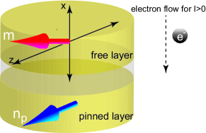
Figure 1: Schematic view of an in-plane magnetized system.

The system we consider is schematically shown in Fig. 1, where the unit vectors pointing in the magnetization directions of the free and the pinned layers are denoted as $\mathbf{m}$ and $\mathbf{n}_{\rm p}=\mathbf{e}_{z}$, respectively. The $z$-axis is parallel to the in-plane easy axis of the free layer while the $x$-axis is normal to the film-plane. The positive current is defined as the electron flow from the free layer to the pinned layer. The energy density of the free layer,

$$E=-MH_{\rm appl}m_{z}-\frac{MH_{\rm K}}{2}m_{z}^{2}+\frac{4\pi M^{2}}{2}m_{x}^{2},$$ (1)

consists of the Zeeman energy, the uniaxial anisotropy energy along the $z$-axis, and the shape anisotropy along the $x$-axis, respectively. The minima of the energy density are $\mp MH_{\rm appl}-(MH_{\rm K}/2)$, corresponding to $\mathbf{m}=\pm\mathbf{e}_{z}$, while the energy density at the saddle point, $\mathbf{m}=(0,\pm\sqrt{1-(H_{\rm appl}/H_{\rm K})^{2}},-H_{\rm appl}/H_{\rm K})$, is $E_{\rm s}=MH_{\rm appl}^{2}/(2H_{\rm K})$. Below, the initial state is taken to be $\mathbf{m}=\mathbf{e}_{z}$. The applied field magnitude $|H_{\rm appl}|$ should be less than $H_{\rm K}$ to guarantee two minima of $E$. The magnetization dynamics is described by the Landau-Lifshitz-Gilbert (LLG) equation,

$$\frac{d\mathbf{m}}{dt}=-\gamma\mathbf{m}\times\mathbf{H}-\gamma H_{\rm s}\mathbf{m}\times\left(\mathbf{n}_{\rm p}\times\mathbf{m}\right)+\alpha\mathbf{m}\times\frac{d\mathbf{m}}{dt},$$ (2)

where $\mathbf{H}=-\partial E/\partial(M\mathbf{m})$. The gyromagnetic ratio and the Gilbert damping constant are denoted as $\gamma$ and $\alpha$, respectively. The spin torque strength,

$$H_{\rm s}=\frac{\hbar\eta I}{2eMV},$$ (3)

includes the spin polarization $\eta$ of the current.

At zero temperature, the initial state becomes unstable when the current magnitude is larger than

$$I_{\rm c}=\frac{2\alpha eMV}{\hbar\eta}\left(H_{\rm appl}+H_{\rm K}+2\pi M\right).$$ (4)

The instability of the initial state does not guarantee the switching. The switching at zero temperature occurs when the current magnitude becomes larger than Hillebrands and Thiaville (2006)

$$I_{\rm c}^{*}=\frac{2\alpha eMV}{\hbar\eta}4\pi M\frac{\mathscr{N}}{\mathscr{D}}.$$ (5)

Here, $\mathscr{N}$ and $\mathscr{D}$ are defined as

$$\begin{split}&\mathscr{N}=\\ &\sqrt{1\!+\!k}[k(1\!+\!k)\!-\!h^{2}]\left\{2(k^{2}\!-\!h^{2})\sqrt{k(1\!+\!k)}\right.\\ &+\left.h\sqrt{k(k^{2}\!-\!h^{2})}\left[\pi+2\sin^{-1}\left(\!\frac{h}{\sqrt{k[k(1+k)\!-\!h^{2}]}}\!\right)\right]\right\},\end{split}$$ (6)

$$\begin{split}&\mathscr{D}=\\ &2h\sqrt{k}(1\!+\!k)(k^{2}\!-\!h^{2})\!+\!k[k(1\!+\!k)\!-\!h^{2}]\sqrt{k(1\!+\!k)(k^{2}\!-\!h^{2})}\\ &\times\!\!\left[\pi+2\sin^{-1}\left(\!\frac{h}{\sqrt{k[k(1+k)\!-\!h^{2}]}}\!\right)\right],\end{split}$$ (7)

where $h=H_{\rm appl}/(4\pi M)$ and $k=H_{\rm K}/(4\pi M)$.

In the thermally activated region $I<I_{\rm c}^{*}$, the magnetization dynamics is described by the Fokker-Planck equation, which can be obtained by adding the stochastic torque, $-\gamma\mathbf{m}\times\mathbf{h}$, to the right hand side of Eq. (2) Jr (1963), and is given by Apalkov and Visscher (2005); Dykman (2012)

$$\frac{\partial\mathcal{P}}{\partial t}+\frac{\partial J}{\partial E}=0,$$ (8)

$$\begin{split}J(E)=&\frac{M}{\gamma}\left(\frac{\mathscr{M}_{\rm s}-\alpha\mathscr{M}_{\alpha}}{\tau}+\frac{MD\mathscr{M}_{\alpha}}{\gamma\tau^{2}}\frac{d\tau}{dE}\right)\mathcal{P}\\ &-D\left(\frac{M}{\gamma}\right)^{2}\frac{\mathscr{M}_{\alpha}}{\tau}\frac{\partial\mathcal{P}}{\partial E},\end{split}$$ (9)

where $\mathcal{P}$ and $J$ are the probability function of the magnetization direction and the probability current, respectively. The diffusion constant $D=\alpha\gamma k_{\rm B}T/(MV)$ relates to the fluctuation-dissipation theorem as $\langle h_{i}(t)h_{j}(t^{\prime})\rangle=(2D/\gamma^{2})\delta_{ij}\delta(t-t^{\prime})$. The functions $\mathscr{M}_{\rm s}(E)=\gamma^{2}H_{\rm s}\oint dt[\mathbf{n}_{\rm p}\cdot\mathbf{H}-(\mathbf{m}\cdot\mathbf{n}_{\rm p})(\mathbf{m}\cdot\mathbf{H})]$ and $\mathscr{M}_{\alpha}(E)=\gamma^{2}\oint dt[\mathbf{H}^{2}-(\mathbf{m}\cdot\mathbf{H})^{2}]$ are proportional to the work done by spin torque and the energy dissipation due to the damping on constant energy line, respectively. The precession period on the constant energy line is denoted as $\tau$. Equation (8) describes the Brownian motion of the magnetization in the effective potential $\mathscr{E}$ defined as

$$\mathscr{E}=\int^{E}dE^{\prime}\left[1-\frac{\mathscr{M}_{\rm s}(E^{\prime})}{\alpha\mathscr{M}_{\alpha}(E^{\prime})}\right].$$ (10)

The steady state solution of Eq. (8) is proportional to $e^{-\mathscr{E}V/(k_{\rm B}T)}$. It should be noted that $I_{\rm c}$ and $I_{\rm c}^{*}$ satisfy $\lim_{E\to-MH_{\rm appl}-(MH_{\rm K}/2)}d\mathscr{E}/dE=1-I/I_{\rm c}$ and $\lim_{E\to E_{\rm s}}d\mathscr{E}/dE=1-I/I_{\rm c}^{*}$, respectively.

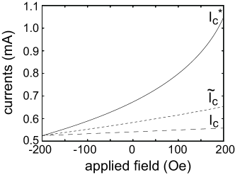
Figure 2: Dependences of $I_{\rm c}$, $\tilde{I}_{\rm c}$, and $I_{\rm c}^{*}$ on the applied field.

The mean first passage time Hänggi et al. (1990), which characterizes how long the magnetization stays in the stable region of the effective potential $\mathscr{E}$, can be introduced as $\mathcal{T}=\int_{0}^{\infty}dt\int_{E^{*}}^{E_{\rm s}}dE_{1}\mathcal{P}(E_{1},t|E^{*},0)$. Here, $E^{*}$ for $I<I_{\rm c}$ is the energy density at the initial state, $-MH_{\rm appl}-(MH_{\rm K}/2)$, while $E^{*}$ for $I_{\rm c}\leq I<I_{\rm c}^{*}$ is determined by the condition $\mathscr{M}_{\rm s}(E^{*})=\alpha\mathscr{M}_{\alpha}(E^{*})$. The solution of the mean first passage time is obtained from Eq. (8), and is given by

$$\begin{split}\mathcal{T}=\frac{\gamma V}{\alpha Mk_{\rm B}T}&\int_{E^{*}}^{E_{\rm s}}dE_{1}\int_{E^{*}}^{E_{1}}dE_{2}\frac{\tau(E_{2})}{\mathscr{M}_{\alpha}(E_{1})}\\ &\times\exp\left\{\frac{[\mathscr{E}(E_{1})-\mathscr{E}(E_{2})]V}{k_{\rm B}T}\right\}.\end{split}$$ (11)

The switching rate from $\mathbf{m}=\mathbf{e}_{z}$ to $\mathbf{m}=-\mathbf{e}_{z}$ is given by $\nu=(1+I/I_{\rm c}^{*})/(2\mathcal{T})$ Taniguchi et al. (2013). In the low-current region $I<I_{\rm c}$ and in the high-barrier limit, the switching rate is

$$\begin{split}\nu=&\frac{\alpha MV\mathscr{M}_{\alpha}(E_{\rm s})}{2\gamma k_{\rm B}T\tau(E^{*})}\left(1-\frac{I}{I_{\rm c}}\right)\left[1-\left(\frac{I}{I_{\rm c}^{*}}\right)^{2}\right]\\ &\times\exp\left[-\Delta_{0}\left(1+\frac{H_{\rm appl}}{H_{\rm K}}\right)^{2}\left(1-\frac{I}{\tilde{I}_{\rm c}}\right)\right],\end{split}$$ (12)

where $\mathscr{M}_{\alpha}(E_{\rm s})=8\pi\gamma M\mathscr{N}/[k^{2}(1+k)^{2}\sqrt{k^{2}-h^{2}}]$ and $\tau(E^{*})=2\pi/[\gamma\sqrt{(H_{\rm appl}+H_{\rm K})(H_{\rm appl}+H_{\rm K}+4\pi M)}]$. The scaling current $\tilde{I}_{\rm c}$ is defined as

$$\tilde{I}_{\rm c}=\frac{2\alpha eMV}{\hbar\eta}\frac{4\pi M}{\mathcal{S}},$$ (13)

where the dimensionless quantity $\mathcal{S}$ is defined as

$$\mathcal{S}=\frac{4\pi M\int_{E^{*}}^{E_{\rm s}}dE^{\prime}\mathscr{M}_{\rm s}(E^{\prime})/\mathscr{M}_{\alpha}(E^{\prime})}{(MH_{\rm K}/2)(1+H_{\rm appl}/H_{\rm K})^{2}H_{\rm s}}.$$ (14)

As mentioned above, Eq. (12) is valid for $I<I_{\rm c}$ and $\Delta=\Delta_{0}(1+H_{\rm appl}/H_{\rm K})^{2}(1-I/\tilde{I}_{\rm c})\gg 1$. The attempt frequency is defined as $f=\nu e^{\Delta}$. On the other hand, in the high-current region $I_{\rm c}\leq I<I_{\rm c}^{*}$, the numerical calculation is necessary to estimate the current dependence of the switching rate $\nu$ Taniguchi et al. (2013).

Figure 2 shows the dependences of $I_{\rm c}$, $\tilde{I}_{\rm c}$, and $I_{\rm c}^{*}$ on the applied field $H_{\rm appl}$. The values of the parameters are $M=1000$ emu/c.c., $H_{\rm K}=200$ Oe, $V=\pi\times 80\times 35\times 2.5$ nm³, $\alpha=0.01$, and $\eta=0.8$, respectively, which are typical values for a magnetic tunnel junction consisting of CoFeB Morota et al. (2008); Yakata et al. (2009); Kubota et al. (2005a, b). The scaling current $\tilde{I}_{\rm c}$ is less than $I_{\rm c}^{*}$, and weakly depends on $H_{\rm appl}$, compared with $I_{\rm c}^{*}$.

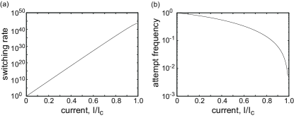
Figure 3: Dependences of (a) the switching rate $\nu$ and (b) the attempt frequency $f$ in the low-current region ($I<I_{\rm c}$) on the current $I$ for $H_{\rm appl}=100$ Oe, where the values of $\nu$ and $f$ are normalized by those at $I=0$ while $I$ is normalized by $I_{\rm c}$

Figures 3 (a) and (b) show the current dependence of the switching rate $\nu$ and the attempt frequency $f$ in the low-current region, $I<I_{\rm c}$. The applied field strength is $H_{\rm appl}=100$ Oe. The current dependence of $\nu$ in the logarithmic scale is approximately linear due to the linear dependence of the switching barrier $\Delta$, although the attempt frequency $f$ also depends on the current. It should be noted that the scaling current of the switching barrier in the low-current region is $\tilde{I}_{\rm c}$, neither $I_{\rm c}$ nor $I_{\rm c}^{*}$ as argued in Refs. Koch et al. (2004); Li and Zhang (2004). This means that the previous analyses of the experiments Morota et al. (2008); Yakata et al. (2009) underestimate the switching current.

In the above formula, the effect of the field like torque Shinjo (2009) is neglected. On the other hand, recently, the effect of the field like torque on the relaxation time, $1/\nu$, was experimentally investigated Rippard et al. (2011), in which the field like torque term is treated as an additional applied field, and is assumed a quadratic function of the bias voltage. From the bias voltage dependence of the relaxation time, the expansion coefficient of the field like torque term was estimated. However, in Ref. Rippard et al. (2011), the attempt frequency ($1/\tau_{0}$ in Ref. Rippard et al. (2011)) is assumed to be independent of the damping constant, temperature, and bias voltage. The combination of our formula developed above with the method in Ref. Rippard et al. (2011) will help the quantitative estimation of the retention time of MRAM with high accuracy.

In summary, the theoretical formula of the spin torque switching rate of an in-plane magnetized system in the presence of an applied field was derived by solving the Fokker-Planck equation. In the low-current region $I<I_{\rm c}$, the current dependence of the switching rate is characterized by three scaling currents, $I_{\rm c}$, $\tilde{I}_{\rm c}$, and $I_{\rm c}^{*}$, where $I_{\rm c}$ and $I_{\rm c}^{*}$ determines the current dependence of the attempt frequency while $\tilde{I}_{\rm c}$ determines that of the switching barrier. The dependences of these scaling currents on the applied field strength were also studied.

The authors would like to acknowledge H. Kubota, H. Maehara, K. Yakushiji, A. Fukushima, K. Ando, and S. Yuasa for the valuable discussions they had with us. This work was supported by JSPS KAKENHI Grant-in-Aid for Young Scientists (B) 25790044.

References

- Albert et al. (2002) F. J. Albert, N. C. Emley, E. B. Myers, D. C. Ralph, and R. A. Buhrman, Phys. Rev. Lett. 89, 226802 (2002).
- Myers et al. (2002) E. B. Myers, F. J. Albert, J. C. Sankey, E. Bonet, R. A. Buhrman, and D. C. Ralph, Phys. Rev. Lett. 89, 196801 (2002).
- Morota et al. (2008) M. Morota, A. Fukushima, H. Kubota, K. Yakushiji, S. Yuasa, and K. Ando, J. Appl. Phys. 103, 07A707 (2008).
- Yakata et al. (2009) S. Yakata, H. Kubota, T. Sugano, T. Seki, K. Yakushiji, A. Fukushima, S. Yuasa, and K. Ando, Appl. Phys. Lett. 95, 242504 (2009).
- Bedau et al. (2010) D. Bedau, H. Liu, J. Z. Sun, J. A. Katine, E. E. Fullerton, S. Mangin, and A. D. Kent, Appl. Phys. Lett. 97, 262502 (2010).
- Jr (1963) W. F. Brown Jr, Phys. Rev. 130, 1677 (1963).
- Koch et al. (2004) R. H. Koch, J. A. Katine, and J. Z. Sun, Phys. Rev. Lett. 92, 088302 (2004).
- Li and Zhang (2004) Z. Li and S. Zhang, Phys. Rev. B 69, 134416 (2004).
- Apalkov and Visscher (2005) D. M. Apalkov and P. B. Visscher, Phys. Rev. B 72, 180405 (2005).
- Shinjo (2009) T. Shinjo, ed., Nanomagnetism and Spintronics (Elsevier, Amsterdam, 2009), chap. 3.
- Butler et al. (2012) W. Butler, T. Mewes, C. Mewes, P. Visscher, W. Rippard, S. Russek, and R. Heindl, IEEE Trans. Mang. 48, 4684 (2012).
- Pinna et al. (2012) D. Pinna, A. Mitra, D. L. Stein, and A. D. Kent, Appl. Phys. Lett. 101, 262401 (2012).
- Pinna et al. (2013) D. Pinna, A. D. Kent, and D. L. Stein, Phys. Rev. B 88, 104405 (2013).
- Kalmykov et al. (2013) Y. P. Kalmykov, W. T. Coffey, S. V. Titov, J. E. Wegrowe, and D. Byrne, Phys. Rev. B 88, 144406 (2013).
- Taniguchi and Imamura (2011) T. Taniguchi and H. Imamura, Phys. Rev. B 83, 054432 (2011).
- Taniguchi and Imamura (2012) T. Taniguchi and H. Imamura, Phys. Rev. B 85, 184403 (2012).
- Taniguchi et al. (2012) T. Taniguchi, M. Shibata, M. Marthaler, Y. Utsumi, and H. Imamura, Appl. Phys. Express 5, 063009 (2012).
- Taniguchi et al. (2013) T. Taniguchi, Y. Utsumi, M. Marthaler, D. S. Golubev, and H. Imamura, Phys. Rev. B 87, 054406 (2013).
- Taniguchi and Imamura (2013) T. Taniguchi and H. Imamura, Appl. Phys. Express 6, 103005 (2013).
- Taniguchi et al. (2013) T. Taniguchi, Y. Utsumi, and H. Imamura, Phys. Rev. B 88, 024414 (2013).
- Hillebrands and Thiaville (2006) B. Hillebrands and A. Thiaville, eds., Spin Dynamics in Confined Magnetic Structures III (Springer, Berlin, 2006), p. 272.
- Dykman (2012) M. Dykman, ed., Fluctuating Nonlinear Oscillators (Oxford University Press, Oxford, 2012), chap. 6.
- Hänggi et al. (1990) P. Hänggi, P. Talkner, and M. Borkovec, Rev. Mod. Phys. 62, 251 (1990).
- Kubota et al. (2005a) H. Kubota, A. Fukushima, Y. Ootani, S. Yuasa, K. Ando, H. Maehara, K. Tsunekawa, D. D. Djayaprawira, N. Watanabe, and Y. Suzuki, Jpn. J. Appl. Phys. 44, L1237 (2005a).
- Kubota et al. (2005b) H. Kubota, A. Fukushima, Y. Ootani, S. Yuasa, K. Ando, H. Maehara, K. Tsunekawa, D. D. Djayaprawira, N. Watanabe, and Y. Suzuki, IEEE Trans. Magn. 41, 2633 (2005b).
- Rippard et al. (2011) W. Rippard, R. Heindl, M. Pufall, S. Russek, and A. Kos, Phys. Rev. B 84, 064439 (2011).