First-order chiral to non-chiral transition in the angular dependence of the upper critical induction of the Scharnberg-Klemm $p$-wave pair state

Abstract

We calculate the temperature $T$ and angular $(\theta,\phi)$ dependence of the upper critical induction $B_{c2}(\theta,\phi,T)$ for parallel-spin superconductors with an axially symmetric $p$-wave pairing interaction pinned to the lattice and a dominant ellipsoidal Fermi surface (FS). For all FS anisotropies, the chiral Scharnberg-Klemm state $B_{c2}(\theta,\phi,T)$ exceeds that of the chiral Anderson-Brinkman-Morel state, and exhibits a kink at $\theta=\theta^{*}(T,\phi)$, indicative of a first-order transition from its chiral, nodal-direction behavior to its non-chiral, antinodal-direction behavior. Applicability to Sr₂RuO₄, UCoGe, and topological superconductors such as Cu_xBi₂Se₃ is discussed.

I Introduction

Recently, there has been a great deal of interest in $p$-wave superconductivityHuy ; deVisser ; HH ; Levy ; Yelland ; Aoki2 ; AokiFlouquet ; SK1985 ; Lorscher ; Mackenzie ; Maeno ; Deguchi ; Machida08 ; Kittaka ; Choi ; Yonezawa ; Suderow ; Machida13 ; FuBerg ; QiZhang ; Kriener ; Bay ; Kirschenbaum ; NLevy . The most likely candidate $p$-wave superconductors are the ferromagnetic superconductors UGe₂, UCoGe, and URhGe, which exhibit long-range ferromagnetism well above the superconducting transition temperature $T_{c}$, and the same electrons participate in the ferromagnetism and the superconductivityHuy ; deVisser ; HH ; Levy ; Yelland ; Aoki2 ; AokiFlouquet . In URhGe, measurements of the temperature $T$ dependence of the upper critical induction $B_{c2}(T)$ in the three crystal axis directions was found to fit the Scharnberg-Klemm theory of the $p$-wave polar state with completely broken symmetry (CBS)HH ; SK1985 , with single-component $p_{z}$-pairing state only along the crystal $a$-axis. Subsequent experiments found a reentrant superconducting phase at much higher magnetic field ${\bm{H}}$ strengths, violating the conventional Pauli limit $B_{P}=1.85T_{c}$ (T/K) by a factor of 20. $B_{c2}$ in UCoGe also violates $B_{P}$ by a factor of 20, but its anisotropy suggests that if the superconductivity were $p$-wave, it would be more likely to have an axial state form, such as do the chiral Anderson-Brinkman-Morel (ABM) and chiral Scharnberg-Klemm (SK) statesAM ; AB ; SK1980 ; Mineev . Second, there has been an even greater interest in Sr₂RuO₄, as the Knight shift measurements for ${\bm{H}}$ parallel and perpendicular to the layers all showed no temperature $T$ dependence below $T_{c}$, suggestive of a parallel-spin stateMackenzie ; Maeno . However, $B_{c2}$ experiments on that material were shown to be strongly Pauli limited for ${\bm{B}}\perp\hat{\bm{c}}$Deguchi ; Machida08 ; Kittaka ; Choi ; Yonezawa ; Machida13 ; Zhang , and scanning tunneling microscopy experiments showed strong evidence for a nodeless gapSuderow , although with cylindrical Fermi surfaces (FSs), this might be consistent with an axial $p$-wave state. Third, there has been a large recent interest in topological insulators, in the hope that they might become chiral $p$-wave superconductors with doping, applied pressure, or proximity couplingFuBerg ; QiZhang ; Kriener ; Bay ; Kirschenbaum ; NLevy . Initial $B_{c2}(T)$ measurements on Cu_xBi₂Se₃ were consistent with a $p$-wave polar state for ${\bm{H}}$ both parallel and perpendicular to the layersBay ; SK1980 . However, scanning tunneling microscopy (STM) experiments established that Cu_xBi₂Se₃ has an isotropic gap strongly suggestive of an $s$-wave order parameter (OP)NLevy , and that isotropic $s$-wave OP was respectively proximity-induced up to 7 K and 50 K into Bi₂Se₃ layers deposited atop the $c$-axes of the layered low-$T_{c}$ and high-$T_{c}$ superconductors, 2$H$-NbSe₂ and Bi₂Sr₂CaCu₂O_8+δShanghai ; Wang , consistent with $s$-wave substrate crystal OPs in the $c$-axis direction of both of those layered superconductorsbook ; Mueller ; Li ; PMReview . However, still undiscovered topological superconductors might have axial $p$-wave OP symmetry.

Previously, we generalized the microscopic calculation of $B_{c2}(T)$ for the $p$-wave polar state pinned to a crystal lattice direction to extend its validity to a superconductor with a dominant ellipsoidal FS and ${\bm{B}}$ in an arbitrary direction, ${\bm{B}}=B(\sin\theta\cos\phi,\sin\theta\sin\phi,\cos\theta)$, with respect to the crystal lattice, in order to provide a sound theoretical basis for a more sensitive probe of the actual OP in orthorhombic materials such as URhGe. Here we use the same technique to construct a theory of the full angular dependence of $B_{c2}(\theta,\phi,T)$ for the ABM and SK states, in order to identify the symmetry of the OP in UCoGe, Sr₂RuO₄, and other candidate materials. Since UCoGe is orthorhombic, the ellipsoidal FS model is the best that can be made without additional features such as magnetic pairing fluctuation effects and ${\bm{B}}$ dependencies of the pairing interactionsHattoriT , or ${\bm{B}}$-dependent interactionsHattoriK , etc. For tetragonal Sr₂RuO₄, the lack of any detectable ferromagnetism strongly suggests weak coupling interactions, but there are three barrel shaped FSs, and the STM experiments strongly suggest nearly equal isotropic gaps on eachSuderow . Although one could envision a scenario in which one FS dominated $B_{c2}(0^{\circ},\phi,T)$ and another dominated $B_{c2}(90^{\circ},\phi,T)$, since the latter is of primary interest, it suffices to consider only one FS. Moreover, as the $k_{z}$ dispersion of those bands is sufficient to avoid dimensional crossover effects in $B_{c2}(90^{\circ},\phi,T)$ measurementsKittaka ; book ; KBL ; KS , an ellipsoid of uniaxial anisotropy is sufficient to examine $B_{c2}$ measurements for all ${\bm{B}}$ directions with high accuracybook . As anticipated earlier, for a parallel-spin pairing interaction of the form $V(\hat{\bm{k}},\hat{\bm{k}}^{\prime})=3V_{0}(\hat{k}_{1}\hat{k}_{1}^{\prime}+\hat{k}_{2}\hat{k}_{2}^{\prime})$, one would expect $B_{c2}(\theta,\phi,T)$ to be given by the SK stateSK1980 ; Lorscher . Although a favorite pair state for Sr₂RuO₄ has the form $\hat{\bm{z}}(\hat{k}_{1}+i\hat{k}_{2})$, where the ${\bm{d}}$-vector $\hat{\bm{z}}$ corresponds to the antiparallel-spin state in the lattice representation, we shall here assume that the spins are parallelSK1980 , and will include Pauli limiting effects subsequentlyZhang . Here we present detailed calculations of the $B_{c2}(\theta,\phi,T)$ for both the ABM and SK states on a single ellipsoidal FS.

We assume weak coupling for a clean homogeneous type-II parallel-spin $p$-wave superconductor with effective Hamiltonian  SK1980 ; Lorscher ,

$$\cal{H} = \sum_{{\bm{k}},\sigma=\pm}a_{{\bm{k}},\sigma}^{{\dagger}}[\epsilon({\bm{k}}-e{\bm{A}})-\mu]a_{{\bm{k}},\sigma}$$ (1)

$$+\frac{1}{2}\sum_{{\bm{k}},{\bm{k}}^{\prime},\sigma}a_{{\bm{k}}^{\prime},\sigma}^{{\dagger}}a_{{\bm{k}},\sigma}^{{\dagger}}V(\hat{\bm{k}},\hat{\bm{k}}^{\prime})a_{{\bm{k}},{\sigma}}a_{{\bm{k}}^{\prime},{\sigma}},$$

$$V(\hat{\bm{k}},\hat{\bm{k}}^{\prime}) = \frac{3}{2}V_{0}\sum_{\sigma^{\prime}=\pm}f_{\sigma^{\prime}}(\hat{\bm{k}})\hat{\bm{d}}_{\sigma^{\prime}}\cdot\hat{\bm{d}}_{\sigma^{\prime}}^{*}f^{*}_{\sigma^{\prime}}(\hat{\bm{k}}^{\prime}),$$ (2)

where we assume parallel-spin pairing with $\hat{\bm{d}}_{\sigma^{\prime}}=\hat{\bm{x}}+i\sigma^{\prime}\hat{\bm{y}}$ and $f_{\sigma^{\prime}}(\hat{\bm{k}})=(\hat{k}_{1}+i\sigma^{\prime}\hat{k}_{2})$ from the degenerate $\Gamma_{3}^{-}$ and $\Gamma_{4}^{-}$ tetragonal point group representationsSigrist , $e$ is the electronic charge, $\mu$ is the chemical potential, the unit wave vectors $\hat{k}_{i}$ were previously defined on an ellipsoidal FSLorscher , and we set $\hbar=k_{B}=1$. For non-ferromagnetic candidate $p$-wave superconductors, the upper critical induction $B_{c2}=\mu_{0}H_{c2}$, where $H_{c2}$ is the upper critical field. After performing the Klemm-Clem (KC) transformationsKC that map the ellipsoidal FS onto a spherical one and then rotate the transformed induction to the new $\tilde{z}$ axis direction, the transformed linear gap equation becomes

$$\overline{\tilde{\Delta}}(\tilde{\bm{R}},\hat{\tilde{\bm{k}}}) = T\sum_{\omega_{n}}\frac{N(0)}{2}\int d\Omega_{\tilde{\bm{k}}^{\prime}}\tilde{V}(\hat{\tilde{\bm{k}}},\hat{\tilde{\bm{k}}^{\prime}})\int_{0}^{\infty}d\xi_{\tilde{\bm{k}}^{\prime}}$$ (3)

$$\times e^{-2\xi_{\tilde{\bm{k}}^{\prime}}|\omega_{n}|}e^{-i\xi_{\tilde{\bm{k}}^{\prime}}v_{F}\hat{\tilde{\bm{k}}^{\prime}}\cdot\tilde{\bm{\Pi}}(\tilde{\bm{R}})}\overline{\tilde{\Delta}}(\tilde{\bm{R}},\hat{\tilde{\bm{k}}^{\prime}}),$$

where $\overline{\tilde{\Delta}}$ is the transformed $\Delta$ amplitude without the gauge phasesLorscher , $N(0)=mk_{F}/(2\pi^{2})$ is the density of states per spin at the chemical potential $\mu$ for an effectively isotropic metal with a geometric mean mass $m=(m_{1}m_{2}m_{3})^{1/3}$, effective Fermi wave vector $k_{F}=\sqrt{2m\mu}$, effective Fermi velocity $v_{F}=k_{F}/m$, and $\tilde{\bm{\Pi}}(\tilde{\bm{R}})=-i\alpha\tilde{\bm{\nabla}}_{\tilde{\bm{R}}}-2e\tilde{\bm{A}}(\tilde{\bm{R}})$, where $\alpha(\theta,\phi)=\sqrt{\overline{m}_{3}}\sqrt{\cos^{2}\theta+\gamma^{-2}(\phi)\sin^{2}\theta}$, $\overline{m}_{i}=m_{i}/m$, and $\gamma^{2}(\phi)=\frac{m_{3}}{m_{1}\cos^{2}\phi+m_{2}\sin^{2}\phi}$ is the ellipsoidal anisotropy functionLorscher . The KC transformations change $V(\hat{\bm{k}},\hat{\bm{k}}^{\prime})$ in Eq. (2) to

$$\tilde{V}(\hat{\tilde{\bm{k}}},\hat{\tilde{\bm{k}}^{\prime}}) = \frac{3}{2}V_{0}\sum_{\sigma=\pm}\tilde{f}_{\sigma}(\hat{\tilde{\bm{k}}})\tilde{f}^{*}_{\sigma}(\hat{\tilde{\bm{k}}}^{\prime})$$ (4)

where $\tilde{f}_{\sigma}(\hat{\tilde{\bm{k}}})=\hat{\tilde{k}}_{1}+i\sigma(\hat{\tilde{k}}_{2}\cos\theta^{\prime}+\hat{\tilde{k}}_{3}\sin\theta^{\prime})$, $\cos\theta^{\prime}=\sqrt{\overline{m}_{3}}\cos\theta/\alpha$, etc.Lorscher From the form of $\tilde{V}(\hat{\tilde{\bm{k}}},\hat{\tilde{\bm{k}}}^{\prime})$, $\overline{\tilde{\Delta}}(\tilde{\bm{R}},\hat{\tilde{\bm{k}}})=\sum_{\sigma=\pm}\overline{\tilde{\Delta}}_{\sigma}(\tilde{\bm{R}})\tilde{f}_{\sigma}(\hat{\tilde{\bm{k}}})$, we expand the $\overline{\tilde{\Delta}}_{\sigma}(\tilde{\bm{R}})$ in terms of the harmonic oscillator eigenfunctions $|n(\tilde{\bm{R}})\rangle$, $\overline{\tilde{\Delta}}_{\sigma}(\tilde{\bm{R}})=\sum_{n=0}^{\infty}a_{n}^{\sigma}|n(\tilde{\bm{R}})\rangle$, perform the integrals over the $\hat{\tilde{k}}_{i}^{\prime}$ variables in the linearized gap equation, and obtain this double recursion relation for the $a^{(\pm)}_{n}$,

$$a_{n}^{(\pm)} = \Bigl{(}\frac{1}{2}(1+\cos^{2}\theta^{\prime})a_{n}^{(\pm)}+\frac{1}{2}\sin^{2}\theta^{\prime}a_{n}^{(\mp)}\Bigr{)}\alpha_{n}^{(a)}$$ (5)

$$+\frac{1}{2}\sin^{2}\theta^{\prime}\Bigl{(}a_{n}^{(\pm)}-a_{n}^{(\mp)}\Bigr{)}\alpha_{n}^{(p)}$$

$$+\Bigl{(}\frac{1}{4}\sin^{2}\theta^{\prime}a_{n+2}^{(\pm)}+\frac{1}{4}(1\pm\cos\theta^{\prime})^{2}a_{n+2}^{(\mp)}\Bigr{)}\beta_{n}$$

$$+\Bigl{(}\frac{1}{4}\sin^{2}\theta^{\prime}a_{n-2}^{(\pm)}+\frac{1}{4}(1\mp\cos\theta^{\prime})^{2}a_{n-2}^{(\mp)}\Bigr{)}\beta_{n-2},$$

where

$$\alpha_{n}^{(p,a)} = \pi T{\sum_{\omega_{n}}}\int_{0}^{\pi}d\theta_{\tilde{\bm{k}}^{\prime}}\sin\theta_{\tilde{\bm{k}}^{\prime}}\left(3\cos^{2}\theta_{\tilde{\bm{k}}^{\prime}},\frac{3}{2}\sin^{2}\theta_{\tilde{\bm{k}}^{\prime}}\right)$$ (6)

$$\times\int_{0}^{\infty}d\xi_{\tilde{\bm{k}}^{\prime}}e^{-2\xi_{\tilde{\bm{k}}^{\prime}}|\omega_{n}|}e^{-\eta_{\tilde{\bm{k}}^{\prime}}/2}L_{n}(\eta_{\tilde{\bm{k}}^{\prime}}),$$

$$\beta_{n} = \pi T\sum_{\omega_{n}}\int_{0}^{\pi}d\theta_{\tilde{\bm{k}}^{\prime}}\frac{3}{2}\mathrm{sin^{3}}\theta_{\tilde{\bm{k}}^{\prime}}\int_{0}^{\infty}d\xi_{\tilde{\bm{k}}^{\prime}}e^{-2\xi_{\tilde{\bm{k}}^{\prime}}|\omega_{n}|}$$ (7)

$$\times e^{-\eta_{\tilde{\bm{k}}^{\prime}}/2}(-\eta_{\tilde{\bm{k}}^{\prime}})L_{n}^{(2)}(\eta_{\tilde{\bm{k}}^{\prime}})[(n+1)(n+2)]^{-1/2},$$

where

$$\eta_{\tilde{\bm{k}}^{\prime}} = eB\alpha(\theta,\phi)v_{F}^{2}\xi^{2}_{\tilde{\bm{k}}^{\prime}}\sin^{2}\theta_{\tilde{\bm{k}}^{\prime}},$$ (8)

$t=T/T_{c}$, $T_{c}=(2e^{C}\omega_{0}/\pi)\exp\left(-1/N(0)V_{0}\right)$, $\omega_{0}$ is a characteristic pairing cutoff frequency, $C\approx 0.5772$ is Euler’s constant, and $L_{n}(z)$ and $L_{n}^{(2)}(z)$ are a Laguerre and an associated Laguerre polynomial, respectivelySK1980 ; Lorscher .

For the chiral ABM state, the decoupled $a_{n}^{(\pm)}$ each satisfy $a_{n}^{(\pm)}D_{n}=\Gamma_{n}a_{n+2}^{(\pm)}+\Gamma_{n-2}a^{(\pm)}_{n-2}$, where $D_{n}=1-\frac{1}{2}(1+\cos^{2}\theta^{\prime})\alpha_{n}^{(a)}-\frac{1}{2}\sin^{2}\theta^{\prime}\alpha_{n}^{(p)}$ and $\Gamma_{n}=\frac{1}{4}\sin^{2}\theta^{\prime}\beta_{n}$. Solving this recursion relation, we obtain the continued fraction expression from which $B_{c2}(\theta,\phi,t)$ for the ABM state is obtained numerically,

$$D_{0}-\frac{\Gamma_{0}^{2}}{D_{2}-\frac{\Gamma_{2}^{2}}{D_{4}-\ldots}} = 0.$$ (9)

As for the polar/CBS stateLorscher , one iteration is accurate to a few percent, but four or five iterations are needed for the accuracy necessary to observe the interesting effects.

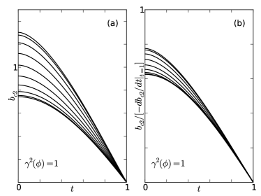
Figure 1: (a) Reduced $b_{c2}$ versus $t=T/T_{c}$ for the chiral ABM state [Eq. (9)] at $\theta$ values from $0^{\circ}$ (${\bm{H}}||\hat{\bm{c}}$, bottom) to $90^{\circ}$ (${\bm{H}}\perp\hat{\bm{c}}$, top), in increments of $10^{\circ}$ for a spherical FS. (b) Same curves normalized to have the same slopes at $T_{c}$.

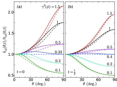
Figure 2: (color online) Reduced $b_{c2}$ versus $\theta$ for the chiral ABM state [Eq. (9)] at the indicated effective mass anisotropy $\gamma^{2}(\phi)$ values (solid) and the effective mass angular fits [Eq. (10), dashed] at $t=0$ (a) and $t=1/2$ (b).

The results for the reduced $b_{c2}(\theta,t)$ for a parallel-spin superconductor in the $p$-wave ABM state with a dominant spherical $\gamma^{2}(\phi)=1$ FS are shown in Fig. 1. In Fig. 1(a), the curves for $\theta=0^{\circ}({\bm{b}}||\hat{\bm{c}})$ (nodal direction) to $90^{\circ}({\bm{b}}\perp\hat{\bm{c}})$ (antinodal direction) are shown in increments of $10^{\circ}$. The result for the nodal direction ($\theta=0^{\circ}$ was obtained previouslySK1980 . Just below $T_{c}$, $b_{c2}(\theta,\phi,t)\propto[m_{3}\cos^{2}\theta+2\gamma^{-2}(\phi)\sin^{2}\theta]^{-1/2}$, where the factor 2 arises from the ABM order parameter (OP) anisotropy. In order to distinguish which part of the overall $b_{c2}(\theta,t)$ anisotropy that is attributable solely to the order parameter anisotropy, in Fig. 1(b), those Fig. 1(a) results scaled to have the same slope at $t=1$ are presented. Nothing unusual is evident from these spherical FS curves, and they are smooth and increase monotonically with increasing $\theta$.

However, we also studied the role of ellipsoidal (or uniaxial) FS anisotropy. In Fig. 2, we chose fixed FS anisotropy values $\gamma^{2}(\phi)$ ranging from 0.1 to 1.5 and plotted in Figs. 1 (a,b) at $t=0$ and $\frac{1}{2}$, respectively. The solid curves are evaluated from Eq. (9). The dashed curves are the conventional “effective mass” anisotropy $b_{\rm eff}(\theta,t)$ forms obtained by fitting the calculated $b_{c2}(0^{\circ},t)$ and $b_{c2}(90^{\circ},t)$,

$$b_{\rm eff}(\theta,t) = [\cos^{2}\theta/b^{2}_{c2}(0^{\circ},t)+\sin^{2}\theta/b^{2}_{c2}(90^{\circ},t)]^{-1/2}.\>\>\>\>\>\>\>$$ (10)

We note that $b_{c2}(\theta,t)$ exhibits an unusual $\theta$ dependence, with a peak in at $\theta^{*}$ for $\gamma^{2}(\phi)<\frac{1}{2}$ that is distinctly different than the conventional $b_{c2}$ maxima at $\theta=0^{\circ}$ or $90^{\circ}$. Such anomalous double peaks at unconventional $\theta$ values satisfying $0<\theta^{*}<90^{\circ}$, and by reflection symmetry about $90^{\circ}$, also for $90^{\circ}<\theta^{*}<180^{\circ}$, were predicted earlier for the polar state pinned to the latticeLorscher . However, in that case, the anomalous double peaks were predicted to occur for $\lambda(t)>\gamma^{2}(\phi)>3$, with maximal $\lambda(t)$ values for finite $t$. Since the anomalous behavior is unlikely to be relevant to either Sr₂RuO₄ or UCoGe, for which $\gamma^{2}\gg 1$, for brevity, the $\lambda^{\prime}(t)$ curve defining the lower limit of the range of $\theta^{*}$ for $\lambda^{\prime}(t)<\gamma^{2}(\phi)<\frac{1}{2}$ will be presented elsewhereZhang .

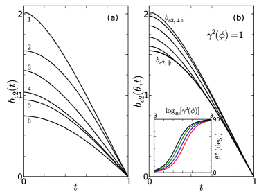
Figure 3: (color online) (a) $b_{c2}(t)$ for the antinodal SK state (1), nodal SK state (2), antinodal ABM state (3), $s$-wave state absent of Pauli limiting (4), planar nodal (CBS) state (5), and nodal ABM state (6) on a spherical FS. (b) Reduced $b_{c2}(t)$ for the chiral SK state at $\theta$ values from $0^{\circ}$ (${\bm{B}}||\hat{\bm{c}}$, bottom) to $90^{\circ}$ (${\bm{B}}\perp\hat{\bm{c}}$, top), in increments of $10^{\circ}$ for a spherical FS. The $\theta=0^{\circ}$, $10^{\circ}$, $20^{\circ}$, $30^{\circ}$ and $40^{\circ}$ are indistinguishable on this scale. Inset: Plots of the kink angle $\theta^{*}$ versus $\log_{10}[\gamma^{2}(\phi)]$ from top to bottom for $t=\frac{3}{4}$ (black), $\frac{1}{2}$ (green), $\frac{1}{4}$ (blue), 0 (red).

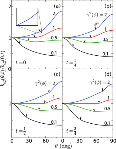
Figure 4: (color online) Reduced upper critical induction $b_{c2}$ versus $\theta$ for the chiral SK state for $\gamma^{2}(\phi)=2$ (blue, top), 1 (red), 0.5 (green), and 0.1 (black) at $t=0$ (a), $\frac{1}{4}$ (b), $\frac{1}{2}$ (c), and $\frac{3}{4}$ (d). The arrows indicate kinks in $b_{c2}(\theta)$ at $\theta^{*}$, signifying first-order transitions from the chiral SK state ($\theta<\theta^{*}$) to the non-chiral antinodal SK (or polar) state $b_{c2}(t)$ curve ($\theta>\theta^{*}$).

The much more interesting chiral axial $p$-wave state is the SK state. We note that it is chiral as long as $\Delta^{(+)}\neq\Delta^{(-)}$, or $a_{n}^{(+)}\neq a_{n}^{(-)}$ for at least one relevant $n$ valueLorscher . It is easy to see that for $\theta^{\prime}=0$, Eq. 5) reduces for $a_{n}^{(+)}\neq 0$ to $[1-\alpha_{n}^{(a)}][1-\alpha_{n+2}^{(a)}]=\beta_{n}^{2}$, which for $a_{n}^{(+)}\neq 0$ is the expression for the SK state with ${\bm{B}}$ in the nodal directionSK1980 , whereas for $\theta^{\prime}=\pi/2$, it reduces for $a_{n}^{(+)}\neq a_{n}^{(-)}$ to $\alpha_{n}^{(p)}=1$, the expression for the SK state with ${\bm{B}}$ in the antinodal (polar state) directionSK1980 .

However, for a general $\theta^{\prime}$, $a_{n}^{(+)}\neq a_{n}^{(-)}$, Eq. (5) is a double recursion relation in the six harmonic oscillator amplitudes, $a_{n}^{(\pm)}$, $a_{n+1}^{(\pm)}$ and $a_{n-2}^{(\pm)}$, which requires further analysis to write the exact solution. We first write $\Psi_{n}^{(\pm)}=\frac{1}{2}(a_{n}^{(+)}\pm a_{n}^{(-)})$, $D_{n}^{(+)}=1-\alpha_{n}^{(a)}$, $D_{n}^{(-)}=1-\alpha_{n}^{(a)}\cos^{2}\theta^{\prime}-\alpha_{n}^{(p)}\sin^{2}\theta^{\prime}$, and construct $\phi_{n}^{(\pm)}=\cos\theta^{\prime}D_{n}^{(+)}\Psi_{n}^{(+)}\pm D_{n}^{(-)}\Psi_{n}^{(-)}$. After letting $n\rightarrow n+2$ in the expression for $\phi^{(-)}_{n}$, we obtain two equations for $\Psi_{n}^{(+)}$ and $\Psi_{n+2}^{(+)}$ in terms of $\Psi_{n}^{(-)}$ and $\Psi_{n+2}^{(-)}$. Using these equations to eliminate $\Psi_{n}^{(+)}$ and $\Psi_{n+2}^{(+)}$ in favor of $\Psi_{n}^{(-)}$ and $\Psi_{n+2}^{(-)}$, letting $n\rightarrow n-2$ in the expression for $\Psi_{n+2}^{(-)}$, and equating that with the other expression for $\Psi_{n}^{(-)}$, we obtain the simple recursion relation for the $\Psi_{n}^{(-)}$, $A_{n}\Psi_{n+2}^{(-)}+B_{n}\Psi_{n}^{(-)}+C_{n}\Psi_{n+2}^{(-)}=0$, the solution of which may be expressed in the continued fraction equation,

$$B_{0}-\frac{A_{0}C_{0}}{B_{2}-\frac{A_{2}C_{2}}{B_{4}-\ldots}} = 0,$$ (11)

where $B_{n}=B_{n}^{(+)}-B_{n}^{(-)}$, $A_{n}=E_{n-2}\beta_{n}[\cos^{2}\theta^{\prime}D_{n+2}^{(+)}-D_{n+2}^{(-)}]$, $B_{n}^{(+)}=D_{n}^{(-)}[E_{n}D_{n-2}^{(+)}+E_{n-2}D^{(+)}_{n+2}]$, $B_{n}^{(-)}=\cos^{2}\theta^{\prime}[\beta^{2}_{n}E_{n-2}+\beta^{2}_{n-2}E_{n}]$, $C_{n}=\beta_{n-2}E_{n}[\beta_{n-2}\cos^{2}\theta^{\prime}D_{n-2}^{(+)}-D_{n-2}^{(-)}]$, and $E_{n}=D_{n}^{(+)}D_{n+2}^{(+)}-\beta_{n}^{2}$. As for the polar/CBS state and the ABM state, one iteration is accurate to a few percent, but four or five iterations are necessary to display the most important features of this work. We also eliminated $\Psi_{n}^{(-)}$ and $\Psi_{n+2}^{(-)}$ in favor of $\Psi_{n}^{(+)}$ and $\Psi_{n+2}^{(+)}$, but the $b_{c2}(\theta,\phi,t)$ values calculated from the resulting continued fraction equation were always lower than those calculated from Eq. (11).

In Fig. 3(a), we plotted the reduced $b_{c2}(t)$ for the nodal and antinodal directions of the ABM, SK, and polar/CBS states, along with that [curve (4)] of a conventional $s$-wave superconductor without any Pauli limiting effects, all for a spherical FS. The antinodal directions of the polar state and SK states both have $b_{c2}(t)$ curves described by curve (1), and the nodal direction of the SK state $b_{c2}(t)$ follows curve (2), as found previouslySK1980 . Curve (3) is the new $b_{c2}(t)$ curve for the antinodal direction of the ABM state. Curves (5) and (6) describe the planar nodal polar/CBS state direction and the nodal direction of the ABM state, as also found previouslySK1985 . We note that the SK state $b_{c2}(\theta,\phi,t)$ is larger for all field directions than is the ABM state $b_{c2}(\theta,\phi,t)$, as the second chiral component of the OP allows for the state to be superconducting at larger applied field strengths. In Fig. 3(b), the $t$ dependence of $b_{c2}(\theta,t)$ is illustrated for $\theta=0^{\circ}({\bm{b}}||\hat{\bm{c}})$ (bottom) to $\theta=90^{\circ}({\bm{b}}\perp\hat{\bm{c}})$ (top), in increments of $10^{\circ}$. Surprisingly, the curves for $\theta=0^{\circ},10^{\circ},20^{\circ},30^{\circ}$ and $40^{\circ}$ are remarkably close to one another, and appear to cross at finite $t$ values! This is an indication of a chiral to non-chiral transition for $\theta\geq 40^{\circ}$ at various $t$ values, as the vortices just below $b_{c2}$ appear to lock onto the nodal direction for $\theta\leq 40^{\circ}$, but for $\theta>40^{\circ}$ unlock from that direction, and favor the non-chiral antinodal (or polar) state direction. Similar behavior was predicted recently for the vortex structure in the mixed state of a chiral ABM state model of Sr₂RuO₄Machida13 .

To investigate this surprising feature in more detail, in Fig. 4 we show the $\theta$ dependence of $b_{c2}(\theta,\phi,t)$ at the effective mass anisotropy values $\gamma^{2}(\phi)=0.1,0.5,1,$ and 2, at $t=0,\frac{1}{4},\frac{1}{2}$, and $\frac{3}{4}$. In every case, there is a kink in $b_{c2}(\theta)$ at $\theta=\theta^{*}$ for fixed $\phi$ and $t$, which we interpret as evidence for a first-order phase transition from a chiral to non-chiral state. Although these kinks are easiest to see for small $\gamma^{2}$ values, and Sr₂RuO₄ has $\gamma^{2}>10^{3}$, our high-accuracy solutions of Eq. (11) allow us to determine $\theta^{*}[\gamma^{2}(\phi),t]$ with great precision. In the inset to Fig. 3(b), we plotted $\theta^{*}$ in degrees versus $\ln_{10}[\gamma^{2}(\phi)]$ from -3 to 3 at the reduced $t$ values 0, $\frac{1}{2},\frac{1}{2}$, and $\frac{3}{4}$. Thus, if Sr₂RuO₄ were a chiral $p$-wave parallel-spin superconductor as often purported, then one ought to observe a first order chiral to non-chiral transition for $\theta\approx 90^{\circ}$, nearly parallel to the layers. It is therefore quite interesting to note that some evidence for this sort of behavior may have already been observed in very recent $H_{c2}(T)$ measurement on Sr₂RuO₄ Yonezawa . However, a cautionary note that is that $b_{c2}(90^{\circ},\phi,t)$ appears to be strongly Pauli limitedKittaka ; Machida08 ; Deguchi ; Choi , and more details of such and other fits using this FS model will soon become availableZhang .

With regards to the ferromagnetic superconductor UCoGe, the ferromagnetism in the $c$-axis direction allows for an axial-type parallel-spin $p$-wave pairing interaction, most likely mediated by ferromagnetic exchange interactions, in the $ab$ plane. However, at large applied fields along the $b$-axis direction, not only does $B_{c2,b}(0)$ exceed the Pauli limit by a factor of at least 20, but the very strange behavior of $B_{c2,b}(T)$, including preliminary evidence for an $S$-shaped curve, strongly suggests something akin to a reentrant superconducting phase overlapping the low-field phase, which would be similar to the two phases of URhGe. Fitting such behavior will require significant modifications to the theory, such as by including ferromagnetic fluctuationsHattoriT , field-dependent interactionsHattoriK , different FS shapes,Youngner ; Rieck , and two ferromagnetically-split FSs, which modifications are currently under studyLorscher2 . Although an axial $p$-wave topological superconductor is presently elusive, this theory could be useful to identify a future candidate material.

In summary, we have studied the two most-common versions of an axially-symmetric $p$-wave pair state, the Anderson-Brinkman-Morel (ABM) and Scharnberg-Klemm (SK) states. For all induction ${\bm{B}}$ directions and temperatures $T$, the reduced (dimensionless) the SK state $B_{c2}(\theta,\phi,t)$ exceeds that of the ABM state. Surprisingly, for $0\leq\theta\leq\theta^{*}$, the only $\theta$-dependence of $B_{c2}(\theta,\phi,t)$ arises from effective mass anisotropy, but then $B_{c2}(\theta)$ exhibits a kink at $\theta^{*}[t,\gamma^{2}(\phi)]$. Hence, it appears that there are two basic states evident in $b_{c2}(\theta,\phi,t)$: the nodal, chiral SK state for $-\theta^{*}\leq\theta\leq\theta^{*}$, and the antinodal, non-chiral polar state for $\theta^{*}\geq\theta\geq-\theta^{*}$.

References

• (1) N. T. Huy et al., Phys. Rev. Lett. 99, 067006 (2007).
• (2) A. de Visser et al., Phys. Rev. Lett. 102, 167003 (2009).
• (3) F. Hardy and A. D. Huxley, Phys. Rev. Lett.94, 247006 (2005).
• (4) F. LΓ©vy, I. Sheikin, and A. Huxley, Nature Phys. 3, 460 (2007).
• (5) E. A. Yelland et al., Nature Phys. 7, 890 (2011).
• (6) D. Aoki et al., J. Phys. Soc. Jpn. 80, 013705 (2011).
• (7) D. Aoki and J. Flouquet, J. Phys. Soc. Jpn. 81, 011003 (2012).
• (8) K. Scharnberg and R. A. Klemm, Phys. Rev. Lett. 54, 2445 (1985).
• (9) C. LΓΆrscher et al., Phys. Rev. B 88, 024504 (2013).
• (10) T. M. Rice and M. Sigrist, J. Phys.: Condens. Matter 7, L643 (1995).
• (11) A. P. Mackenzie and Y. Maeno, Rev. Mod. Phys. 75, 657 (2003).
• (12) Y. Maeno et al., J. Phys. Soc. Jpn. 81, 011009 (2012)
• (13) K. Deguchi, Z. Q. Mao, and Y. Maeno, J. Phys. Soc. Jpn. 73, 1313 (2004).
• (14) K. Machida and M. Ichioka, Phys. Rev. B 77, 184515 (2008).
• (15) S. Kittaka et al., Phys. Rev. B 80, 174514 (2009).
• (16) C.-H. Choi, J. Kor. Phys. Soc. 56, 933 (2010).
• (17) S. Yonezawa, T. Kajikawa, and Y. Maeno, Phys. Rev. Lett. 110, 077003 (2013).
• (18) H. Suderow et al., New. J. Phys. 11, 093004 (2009).
• (19) M. Ishihara et al., Phys. Rev. B 87, 224509 (2013).
• (20) L. Fu and E. Berg, Phys. Rev. Lett. 1Ν‘05, 097001 (2010).
• (21) X. L. Qi and S. C. Zhang, Rev. Mod. Phys. 83, 1057 (2011).
• (22) M. Kriener et al., Phys. Rev. Lett. 106, 127004 (2011).
• (23) T. V. Bay et al., Phys. Rev. Lett. 108, 057001 (2012).
• (24) K. Kirschenbaum et al., Phys. Rev. Lett. 111, 087001 (2013).
• (25) N. Levy et al., Phys. Rev. Lett. 110, 117001 (2013).
• (26) K. Scharnberg and R. A. Klemm, Phys. Rev. B 22, 5233 (1980).
• (27) P. W. Anderson and P. Morel, Phys. Rev. 123, 1911 (1961).
• (28) P. W. Anderson and W. F. Brinkman, Phys. Rev. Lett. 30, 1108 (1973).
• (29) V. P. Mineev and K. V. Samokhin, Introduction to Unconventional Superconductivity (Gordon and Breach, New York, NK, 1999).
• (30) J. Zhang et al., to be published.
• (31) R. A. Klemm, Layered Superconductors Volume 1 (Oxford University Press, Oxford, UK and New York, NY 2012).
• (32) M. Wang et al., Science 336, 52 (2012).
• (33) E. Wang et al., Nat. Phys. 9, 620 (2013).
• (34) K. A. Mueller, BAPS.2011.MAR.J3.2
• (35) Q. Li et al., Phys. Rev. Lett. 83, 4160 (1999).
• (36) R. A. Klemm, Phil. Mag. 85, 801 (2005).
• (37) T. Hattori et al., Phys. Rev. Lett. 108, 066403 (2012).
• (38) K. Hattori and H. Tsunetsugu, Phys. Rev. B 87, 064501 (2013).
• (39) R. A. Klemm, A. Luther, and M. R. Beasley, Phys. Rev. B 12, 877 (1975).
• (40) R. A. Klemm and K. Scharnberg, Phys. Rev. B 24, 6361 (1981).
• (41) R. A. Klemm and J. R. Clem, Phys. Rev. B 21, 1868 (1980).
• (42) E. Helfand and N. R. Werthamer, Phys. Rev. 147, 288 (1966).
• (43) D. W. Youngner and R. A. Klemm, Phys. Rev. B 21, 3890 (1980).
• (44) C. T. Rieck and K. Scharnberg, Physica B 163, 670 (1990).
• (45) C. LΓΆrscher et al., unpublished.