Cold stream stability during minor mergers

Abstract

We use high-resolution Eulerian simulations to study the stability of cold gas flows in a galaxy size dark matter halo ($10^{12}\hbox{$\rm\thinspace M_{\odot}$}$) at redshift $z=2$. Our simulations show that a cold stream penetrating a hot gaseous halo is stable against thermal convection and Kelvin-Helmholtz instability. We then investigate the effect of a satellite orbiting the main halo in the plane of the stream. The satellite is able to perturb the stream and to inhibit cold gas accretion towards the center of the halo for 0.5 Gyr. However, if the supply of cold gas at large distances is kept constant, the cold stream is able to re-establish itself after 0.3 Gyr. We conclude that cold streams are very stable against a large variety of internal and external perturbations.

1 Introduction

How do galaxies get their gas is a key question to better understand their formation and evolution. In the conventional picture, the cold gas is accreted onto the Dark Matter halo, and is shock heated to the virial temperature of the halo. The hot gas then loses pressure support due to radiative cooling, then settles into a centrifugally supported disc and begins to form stars (Fall & Efstathiou, 1980; White & Frenk, 1991). This picture has been supported by early simulations which have shown that a substantial fraction of cold gas was indeed shock heated after accretion (Benson et al., 2001; Helly et al., 2003).

A number of theoretical and simulation-based works in the past decade, however, have found two distinct modes of gas accretion, named as hot and cold accretion (Birnboim & Dekel, 2003; Kereš et al., 2005; Dekel & Birnboim, 2006; Kereš & Hernquist, 2009; Dekel et al., 2009). Cold gas flowing along dark matter filaments can be directly accreted onto the central galaxy without being shock heated, cold streams are the main source of gas supply in galaxies especially in low-mass halos of $M_{h}\leq 10^{12}\hbox{$\rm\thinspace M_{\odot}$}$ at high redshift (Dekel et al., 2009).

Simulations also predict that these cold streams, being optically thick Lyman-limit systems with low metallicities, could be observable via absorption lines against background-objects (Fumagalli et al., 2011). Stewart et al. (2010) proposed that cold-flow streams will produce an orbiting circum-galactic component of cool gas with high angular momentum, which might be observable as well. However, the existence of cold streams has not been confirmed by solid observational results. Observations from Steidel et al. (2010), showed outflow rather than inflow of cold gas in the circum-galactic medium . Faucher-Giguère & Kereš (2011) argued that the covering factor might be smaller than $10\%-20\%$ at $z=2$, so the observation of cold streams is very difficult. Very recently, several observations (Bouchè et al., 2013; Crighton et al., 2013) reported distinct signatures of strong metal poor absorbing systems in the vicinity of galaxies at $z\sim 2.3-2.4$ by observing background quasars. Features of these systems are broadly consistent with the prediction of accreted cold gas in simulations. However, to confirm the existence of cold streams, information on the morphology of the cold gas is needed.

If cold streams do appear at some epoch, the velocity shear between them and hot gas will drive Kelvin-Helmholtz (K-H) instability. When the contact surface between cold and hot gas is not aligned with the gravity gradient, Rayleigh-Taylor (R-T) instability will also grow. In addition, thermal evaporation will occur. Another source of instability for the cold flows may come from the very high merger rate of dark matter haloes predicted in the hierarchical scenario, especially at high redshift (Fakhouri et al., 2010). All these possible sources of perturbation naturally raise the question: how long could the cold streams survive against such instabilities?

In this Letter we make a first attempt in trying to determine the stability of cold flows. We employ high resolution hydrodynamical Eulerian simulations combined with a simplified set-up that allows us to better understand the impact of all these different sources of instability. The Letter is organized as follows: We present our numerical methods and cold flow model in §2. Hydrodynamical simulation results are shown in §3. Discussion and conclusion are given in §4.

2 Initial parameters set-up and numerical simulations

We assume that the cold streams are penetrating through a hot gaseous halo which is in hydrostatic equilibrium with the gravitational potential of the hosting dark matter halo. The dark matter halo has a mass of $M_{h}=10^{12}M_{\odot}$ and we assume a NFW profiles (, 1997) with a concentration parameter of 10 following Macciò et al. (2008). All the cosmological parameters are set in agreement with the WMAP5 results (Komatsu et al., 2009).

2.1 Hot gaseous halo

The hot halo gas is initially set to be isothermal and in hydrostatic equilibrium under the gravitational potential of the dark matter halo. The self gravity of gas is not included. The central (stellar) galaxy component is not considered as we are mainly interested in the hydrodynamical evolution of cold streams within the virial radius. The temperature of the hot halo is set to $T_{halo}\sim 3.3\times 10^{6}{\rm\thinspace K}$, and we assume a poly-tropic index $\gamma=5/3$ polytropic. Finally we extend the gas distribution to 1.5 times the virial radius of the dark matter halo, (to what we call the boundary radius $R_{b}\equiv 1.5R_{h}$), in order to reduce any possible boundary effect. The hot gas accounts for $17\%$ of the total mass within $R_{h}$.

2.2 Cold stream

The morphology, temperature, density and velocity of cold streams are set according to recent theoretical and simulation works (Dekel et al., 2009; Ocvirk et al., 2008; van de Voort & Schaye, 2012). van de Voort & Schaye (2012) performed a very broad statistical study of the cold streams velocity and temperature as function of distance from the halo center for dark matter haloes with $10^{11.5}<M_{h}<10^{12.5}\hbox{$\rm\thinspace M_{\odot}$}$ at $z=2$. According to their results we assume the velocity of cold streams at $R_{b}$ to be $v_{cold}(R_{b})\sim 100\hbox{${\rm\thinspace km}{\rm\thinspace s}^{-1}\,$}$.

The cold stream is firstly assumed to be a simple cone geometry, following simulations results (Dekel et al., 2009; Kereš & Hernquist, 2009). The radius of the stream at the boundary $R_{b}$ is given by

$$R_{cold}(R_{b})\sim R_{b}\times\sin(\frac{\theta}{2})$$ (1)

where $\theta$ is the stream opening angle and could be derived from the covering factor $\eta$ as $\theta\sim 2\pi\eta/x_{cold}$, where $x_{cold}$ is the number of cold streams in the halo, we adopt the value of $x_{cold}=3$(Danovich et al., 2012). On the other hand the covering factor $\eta$ is more difficult to estimate. Dekel et al. (2009) predicted that gas at temperature $<10^{5}{\rm\thinspace K}$ with column densities $>10^{20}{\rm\thinspace cm}^{-2}$ should cover $\sim 25\%$ the area at radii from 20 to 100 kpc in haloes with $M_{h}\sim 10^{12}\hbox{$\rm\thinspace M_{\odot}$}$ at $z\sim 2.5$. Faucher-Giguère & Kereš (2011) measured the covering factor for a Milky Way type progenitor Lyman-break galaxy in a cosmological simulation and found a smaller value, which is $\sim 10\%$ for the Lyman limit systems and $\sim 3\%$ for the damped Ly$\alpha$ absorbers within $R_{h}$. We adopt a value of $20\%$ within $R_{b}$, in agreement with recent studies by Goerdt et al. (2012); Fumagalli et al. (2013). Therefore, $R_{cold}(R_{b})\sim 15{\rm\thinspace kpc}$.

The density of cold gas $\rho_{cold}$ at $R_{b}$ can be determined by the accretion rate $\dot{M}(R_{b},t)$, $R_{cold}(R_{b})$, the velocity and the mass ratio of cold accretion mode as,

$$\rho_{cold}(R_{b})=f_{cold}\frac{\dot{M}}{x_{cold}v_{cold}(R_{b})\pi R^{2}_{cold}(R_{b})}$$ (2)

where, $f_{cold}$ is the cold accreted gas mass fraction. Using the so called extended Press & Schechter approach (Lacey & Cole, 1994) for structure formation, Dekel et al. (2009) derived that the growth rate of the baryonic mass at the virial radius should be

$$\dot{M}\simeq 6.6\times M^{1.15}_{12}(1+z)^{2.25}f_{.165}~{}~{}\hbox{$\rm\thinspace M_{\odot}$}{\rm\thinspace yr}^{-1}$$ (3)

where $M_{12}\equiv M_{h}/10^{12}\hbox{$\rm\thinspace M_{\odot}$}$, and $f_{.165}$ is the baryonic fraction in the haloes in units of the cosmic mean. For a halo with $M_{h}=10^{12}\hbox{$\rm\thinspace M_{\odot}$}$, it is about $\dot{M}\simeq 80\hbox{$\rm\thinspace M_{\odot}$}{\rm\thinspace yr}^{-1}$ at $z=2$. However, van de Voort & Schaye (2012) found a mean value of $\sim 30\hbox{$\rm\thinspace M_{\odot}$}{\rm\thinspace yr}^{-1}$ and $\sim 20\hbox{$\rm\thinspace M_{\odot}$}{\rm\thinspace yr}^{-1}$ for the total and cold baryonic mass accretion respectively.

For our selected cold accretion rate, $f_{cold}\times\dot{M}=20\hbox{$\rm\thinspace M_{\odot}$}{\rm\thinspace yr}^{-1}$, and the number of cold streams, $x_{cold}=3$, the net accretion rate for one single cold stream is $7\hbox{$\rm\thinspace M_{\odot}$}{\rm\thinspace yr}^{-1}$. In our simulation we only model one such cold stream. The density of the cold stream at the boundary, $R_{b}$ is $\sim 3.0\times 10^{-26}{\rm\thinspace g}{\rm\thinspace cm}^{-3}$ obtained from Eq.2. The temparature of cold gas is set to $T_{cold}(R_{b})=3.3\times 10^{4}{\rm\thinspace K}$, which is almost in thermal pressure quilibrium. In Fig.1 we give a schematic of the initial condition, and the simulation parameters are listed in table 1.

2.3 Orbiting satellite

The satellite is described by a single, mass varying particle with an initial mass of $3\times 10^{10}$ $\rm\thinspace M_{\odot}$, leading to a merger mass ratio of 1/33. The orbit of the satellite is predetermined and extracted from a similar high resolution N-body simulation in Chang et al. (2013). The initial position of the satellite is at $R_{b}$, locating at the opposite side of the cold accretion with respect to the halo center. The initial radial and tangential velocity of the satellite are respectively set to $0.9$ and $0.6$ times of the virial velocity of the main halo, $v_{vir}=160\hbox{${\rm\thinspace km}{\rm\thinspace s}^{-1}\,$}$.The mass evolution of the satellite is also extracted, giving $1.4\times 10^{10}\hbox{$\rm\thinspace M_{\odot}$}$ at 2 Gyr.

Finally we assume the orbit plane of the satellite is co-planar with the cold stream plane. Such a choice is motivated by results from N-body simulations (Zentner, Kravtsov, & Gnedin et al., 2005), and by recent observation of a possible “cosmic alignment” of galactic satellites in M31 (Ibata et al., 2013). A sketch of our initial configuration and the satellite orbit are presented in Figure 1.

Table 1: Parameters used in the hydrodynamic simulation

halo concentration (c)	10
virial radius ($R_{h}$)	$100{\rm\thinspace kpc}$
virial mass ($M_{h}$)	$10^{12}\hbox{$\rm\thinspace M_{\odot}$}$
hot gas central density ($\rho_{hot}$)	$3.0\times 10^{-24}{\rm\thinspace g}{\rm\thinspace cm}^{-3}$
hot gas temperature ($T_{hot}$)	$3.3\times 10^{6}{\rm\thinspace K}$
boundary radius $R_{b}$	$150{\rm\thinspace kpc}$
cold gas density at $R_{b}$ ($\rho_{cold}(R_{b})$)	$3.0\times 10^{-26}{\rm\thinspace g}{\rm\thinspace cm}^{-3}$
cold gas velocity at $R_{b}$ ($v_{cold}(R_{b})$)	$100\hbox{${\rm\thinspace km}{\rm\thinspace s}^{-1}\,$}$
cold gas temperature at $R_{b}$ ($T_{cold}(R_{b})$)	$4.0\times 10^{4}{\rm\thinspace K}$
cold gas pressure at $R_{b}$	$10^{-15}{\rm\thinspace erg}{\rm\thinspace cm}^{-3}$

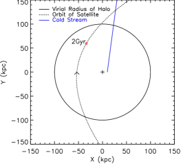
Figure 1: The sketch map of our simulation. The solid black circle is the virial radius of dark matter halo, the blue sold line is the axis of injected cold stream at $R_{b}$, the dashed curve is the orbit of the satellite and the red circle mark the position of the satellite at 2 Gyrs.

2.4 Numerical methodology

To track the evolution of cold streams, we run hydrodynamical simulations with a fixed grid code using the positive preserving WENO scheme (Zhang & Shu, 2010), which can effectively keep positive density and pressure in hypersonic regions, and can well capture the motions of the baryonic gas in cosmological simulations (Zhu, Feng, & Xia et al, 2013). Simulations are performed in a cubic box of 300 kpc, with a number of grid cells $512^{3}$, i.e, a resolution of $0.59$ ${\rm\thinspace kpc}$. Analytical gravitational potentials based on NFW profiles are given at each grid cell initially. We impose hydrostatic equilibrium for the boundary condition except for the stream. Density and velocity in the ghost grid cells outside the boundary of the simulation box are assumed to be zero-gradient along the radial direction and the pressure is given by a first-order differentiation of the hydrostatic equilibrium equation.

Radiative cooling is followed by using the cooling function given in Sutherland & Dopita (1993). Recent simulation works (van de Voort & Schaye, 2012; Ocvirk et al., 2008) showed that the metallicity abundance ranges from $\sim 10^{-1}$ to $10^{-3}$ $Z_{\odot}$ for the cold gas. We adopt the value $\sim 10^{-1.5}Z_{\odot}$, and further assume the hot gas has the same value for the sake of simplicity. Thermal conduction is also included with the unsaturated regime assumption, and the thermal conductivity is set to $\kappa(T)=\kappa_{0}T^{5/2}$ (Spitzer, 1962), with $\kappa_{0}\simeq 1.84\times 10^{-5}(\ln\Lambda)^{-1}{\rm\thinspace erg}{\rm\thinspace s}^{-1}{\rm\thinspace cm}^{-1}{\rm\thinspace K}^{-7/2}$, where $\ln\Lambda$ is the Coulomb logarithm, which is only weakly dependent on $n_{e}$ and $T$ ($\ln\Lambda=30$ in our simulation).

From our model set up, the cold gas is injected into the simulation box within an aperture radius of $15$ kpc at $R_{b}$ with a constant rate of $7\hbox{$\rm\thinspace M_{\odot}$}{\rm\thinspace yr}^{-1}$, with the density, velocity and temperature given in Table.1. The constant inflow rate lasts for the whole simulation run, i.e., 4 Gys. It is found that a stable cold stream towards the halo central region is soon established under the gravity of the host halo, with time less than 1.5 Gyr (top left panel of Fig.2). Note that for the cold stream we assume an impact parameter $b\sim 30{\rm\thinspace kpc}$ respect to the halo center, as suggested by cosmological simulations (Dekel et al., 2009; Kereš & Hernquist, 2009).

We perform two sets of simulations, with and without the inclusion of the merging satellite, which are referred to as col-mer-512 and col-ref-512 respectively. The latter simulation is intended to track the effect of thermal conduction and K-H instability, while the former is used to study the impact of an orbiting satellite on the stability of cold flows.

3 Simulation Results

Fig. 2 presents the slices of density and temperature distribution of gas at 1.5, 2.5, 3.0 and 4.0 Gyrs in the simulations without/with the satellite in the upper/lower panels, respectively. The evolution before 1.5 Gyrs, during the formation of the stream, is practically the same in the two simulations and it is not shown.

In the simulation without satellite, only subtle changes in morphology, density and temperature happen to the stream after its formation. Thermal conduction results a thin transition layer between the two gas phases and evidence for K-H instability is hard to find. The cold gas could flow into the central region ($<0.3R_{h}$) with a velocity as high as $400\hbox{${\rm\thinspace km}{\rm\thinspace s}^{-1}\,$}$. After passing through the inner region, a small fraction of gas flows out of $0.5R_{h}$. In a full cosmological simulation this gas will be retained by the central galaxy and used for star formation.

In the col-mer-512 simulation, obvious disturbances have been triggered by the satellite at 2.5 and 3.0 Gyrs. There is practically no flow of cold gas inside $0.5R_{h}$ at 3.0 Gyr. Interestingly enough the cold stream is re-established after 4.0 Gyr, when the satellite is far away from the stream.

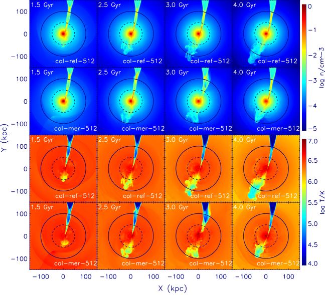
Figure 2: The top two rows are density slices of the col-ref-512 and col-mer-512 simulations, (1st and 2nd row respectively). Each column represents 1.5, 2.5, 3.0 and 4.0 ${\rm\thinspace Gyrs}$. The bottom two rows are temperature slices. The solid/dashed line indicates the virial radius $R_{h}$/0.5$R_{h}$. At $t=1.5$ Gyr the radius of the stream at $R_{h}$ and $0.5R_{h}$ is around 7.5 and 5 kpc respectively.

In order to quantify the effect of satellite on the cold stream, we present in Fig. 3 the evolution of the net accretion rate of cold gas through a spherical shell at $R_{h}$ and at $0.5R_{h}$. Gas with temperature below $3\times 10^{5}$ K is defined as cold. The col-ref-512 run shows an almost constant accretion rate at both radius. This implies that thermal conduction and gravitational heating are able to convert only a small fraction of the incoming cold gas to the hot phase.

The situation is very different for the col-mer-512 run. The accretion rate at both radius shows sharp drops delayed by a couple of hundred Myr with respect to the crossing of the stream by the satellite. The accretion rate at at 0.5 $R_{h}$ is practically suppressed for a period of $\sim 0.5$ Gyrs. This very reduced cold accretion is clearly connected with the close passage of the satellite at $t=2.5$ Gyrs, marked by the red line in the figure.

Despite the very destructive effect of the satellite on the stream, the cold flow is able to re-build itself quite rapidly in less than 0.3 Gyrs. This shows that in the presence of a continuous accretion of cold gas from cosmological filaments, even if disturbed by orbiting satellites, cold flows are able to regenerate themselves quite rapidly.

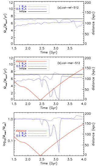
Figure 3: The evolution of the cold gas accretion rate. Top/Middle panel: for the simulation without/with a merging satellite with a 1:33 mass ratio. Bottom panel: the ratio of gas accretion between the two simulation runs. The black line indicates the cold gas inflow rate at the boundary of the simulation box ($1.5R_{h}$). In the middle and bottom panels, the red line indicate the distance between the satellite and the cold stream.

4 Discussion and Conclusion

In this letter, inspired by recent simulation works and observations, we have studied the stability of cold streams penetrating through hot gaseous halos in dark matter halos with mass $M=10^{12}M_{\odot}$ at $z=2$ by hydrodynamic simulations in a simplified scenario.

Without external perturbations (e.g. satellites), the cold gas is able to flow into the inner region of the central galaxy. The K-H instability and thermal conduction are not able to inhibit the cold gas accretion. K-H instability might have been damped by the supersonic motion of the gas due to the low cooling rate (Vietri et al., 1997).

When we consider the disturbing action of a satellite (with a mass ratio of 1:33) merging with the central halo, the accretion rate of cold gas at half of the virial radius experiences a dramatic drop for $\sim$ 0.5 Gyrs. In this period the supply of cold gas into the central region decreases by more than $\sim 70\%$.

Cosmological simulations have shown that the merger rate at $z=2$ for our satellite/host mass combination is about two mergers per Gyr(Fakhouri et al., 2010). However, the cross section between isotropically distributed stream and satellites can be crudely estimated by

$$\frac{V_{cs}}{V_{halo}}=\left(R_{cold}\right)^{2}2\pi\frac{R_{h}}{3}/\frac{4\pi}{3}R_{h}^{3}\sim 1\%$$ (4)

where $V_{cs}$ and $V_{halo}$ are the volume of cold stream and halo respectively. Therefore, the realistic distribution of cold stream and satellite would play an important role.

Even in the case of a direct interaction between the satellite and the stream, the flow of cold gas towards the halo center is able to re-establish itself in less than 0.3 Gyrs, under the assumption of a continuous flow of cold gas from cosmic filaments.

What we present in this Letter is a pilot study for the stability of Cold Flows. We plan to improve and extend it in forthcoming works by increasing the resolution of the simulation, considering different satellite orbits and impact parameters, adding the self gravity of the gas and comparing different hydrodynamical approaches (see Nelson et al. (2013) for the effect of the hydro solver on the cold flow stability in cosmological simulations). Meanwhile, we expect that further observations may reveal more information about both cold and hot gas in the halo, and more details on galaxy formation and growth.

References

- Benson et al. (2001) Benson A.J., Frenk C.S., Baugh C.M., Cole S., Lacey C.G., 2001, MNRAS, 327, 1041
- Birnboim & Dekel (2003) Birnbiom Y., Dekel A., 2003, MNRAS, 345, 349
- Bouchè et al. (2013) Bouchè N., Murphy M.T. et al., 2013, Science, 341, 50
- Chang et al. (2013) Chang J., Macciò A.V., Kang X., 2013, MNRAS, 431, 3533
- Crighton et al. (2013) Crighton N., Hennawi J., Prochaska J., 2013, ApJL, 776, L18
- Danovich et al. (2012) Danovich M., Dekel A., Hahn O., Teyssier R., 2012, MNRAS, 422, 1732
- Dekel & Birnboim (2006) Dekel A., Birnbiom Y., 2006, MNRAS, 368, 2
- Dekel et al. (2009) Dekel A., Birnbiom Y.,Engel G. et al., 2009, Nature, 457, 451
- Fall & Efstathiou (1980) Fall S.M., Efstathiou G., 1980, MNRAS, 193, 189
- Fakhouri et al. (2010) Fakhouri O., Ma, C-P., Boylan-Kolchin M., 2010, MNRAS, 406, 12
- Faucher-Giguère & Kereš (2011) Faucher-Gifuère C.A., Kereš D., 2011, MNRAS, 412, L118
- Fumagalli et al. (2011) Fumagalli M., Prochaska J., Kasen D., Dekel A., Ceverino D., Primack J. R., 2011, MNRAS, 418, 1796
- Fumagalli et al. (2013) Fumagalli M., ÒMeara J. M., Prochaska J. X., Worseck G., 2013, ApJ, 775, 78
- Goerdt et al. (2012) Goerdt T., Dekel A., Sternberg A., Gnat O., Ceverino D., 2012, MNRAS, 424, 2292
- Helly et al. (2003) Helly J.C., Cole S., Frenk C.S., Baugh C.M., Benson A., Lacey C., Pearce F.R., 2003, MNRAS, 338, 913
- Ibata et al. (2013) Ibata R.A., Lewis G.F. et al., 2013, Nature, 2013, 493, 62
- Kereš et al. (2005) Kereš D., Katz N., Weinberg D.H., Dave R., 2005, MNRAS, 363, 2
- Kereš & Hernquist (2009) Kereš D., Hernquist L., 2009, ApJ, 700, L1
- Komatsu et al. (2009) Komatsu, E., Dunkley, J., Nolta, M. R., et al. 2009, ApJS, 180, 330
- Lacey & Cole (1994) Lacey C., Cole S., 1994, MNRAS, 271, 676
- Macciò et al. (2008) Macciò, A. V., Dutton, A. A., & van den Bosch, F. C. 2008, MNRAS, 391, 1940
- (22) Navarro, J. F., Frenk, C. S., & White, S. D. M. 1997, ApJ, 490, 493
- Nelson et al. (2013) Nelson, D., et al. 2013, MNRAS, 429,3353
- Ocvirk et al. (2008) Ocvirk P., Pichon C., Teyssier R., 2008, MNRAS, 390, 1326
- Spitzer (1962) Spitzer L., 1962, Physics of Fully Ionized Gases (New York: Interscience)
- Steidel et al. (2010) Steidel C., Erb D. Shapley A. et al., 2009, ApJ, 700, L1
- Stewart et al. (2010) Stewart K.R., Kaufmann T., Bullock J.S., Barton E.J., et al., 2011, ApJ, 738, 39
- Sutherland & Dopita (1993) Sutherland R.S., Dopita M.A., 1993, ApJS, 88, 253
- Vietri et al. (1997) Vietri M., Ferrara A., Miniati F., 1997, ApJ, 483, 262
- White & Frenk (1991) White Simon D. M., Frenk Carlos S., 1991, ApJ, 52, 379
- van de Voort & Schaye (2012) van de Voort F., Schaye J., 2012, MNRAS, 423, 2991
- Zentner, Kravtsov, & Gnedin et al. (2005) Zentner A. R., Kravtsov A. V., Gnedin O. Y., Klypin A. A., 2005, ApJ, 629, 219
- Zhang & Shu (2010) Zhang X., Shu C.W., 2010, Journal of Computational Physics, 229, 8918
- Zhu, Feng, & Xia et al (2013) Zhu, W.S., Feng, L.L., Xia, Y.H., Shu, C.-W., Gu, Q.S., & Fang, L. Z., 2013, ApJ, 777, 48