Galactic and Circumgalactic O VI and Its Impact on the
Cosmological Metal and Baryon Budgets at $2<z\mathrel{\hbox{\hbox to0.0pt{\hbox{\lower 4.0pt\hbox{$\sim$}}\hss}\hbox{$<$}}}3.5$

Abstract

We present the first results from our NASA Keck Observatory Database of Ionized Absorbers toward Quasars (KODIAQ) survey which aims to characterize the properties of the highly ionized gas of high redshift galaxies and their circumgalactic medium (CGM) at $2<z<4$. We select absorbers optically thick at the Lyman limit ($\tau_{\rm LL}>1$, $\log N_{\rm HI}>17.3$) as probes of these galaxies and their CGM where both transitions of the O VI doublet have little contamination from the Ly $\alpha,\beta$ forests. We found 20 absorbers that satisfy these rules: 7 Lyman limit systems (LLSs), 8 super-LLSs (SLLSs) and 5 damped Ly$\alpha$ (DLAs). The O VI detection rate is 100% for the DLAs, 71% for the LLSs, and 63% for the SLLSs. When O VI is detected, $\log\langle N_{\rm OVI}\rangle=14.9\pm 0.3$, an average O VI column density substantially larger and with a smaller dispersion than found in blind O VI surveys at similar redshifts. Strong O VI absorption is therefore nearly ubiquitous in the CGM of $z\sim 2$–$3$ galaxies. The total velocity widths of the O VI profiles are also large ($200\leq\Delta v_{\rm OVI}\leq 400$ ${\rm km\,s}^{-1}$). These properties are quite similar to those seen for O VI in low $z$ star-forming galaxies, and therefore we hypothesize that these strong CGM O VI absorbers (with $\tau_{\rm LL}>1$) at $2<z\mathrel{\hbox{\hbox to0.0pt{\hbox{\lower 4.0pt\hbox{$\sim$}}\hss}\hbox{$<$}}}3.5$ also probe outflows of star-forming galaxies. The LLSs and SLLSs with no O VI absorption have properties consistent with those seen in cosmological simulations tracing cold streams feeding galaxies. When the highly ionized (Si IV and O VI) gas is taken into account, we determine that the $\tau_{\rm LL}>1$ absorbers could contain as much as 3–14% of the cosmic baryon budget at $z\sim 2$–3, only second to the Ly$\alpha$ forest. We conservatively show that $5$–$20\%$ of the metals ever produced at $z\sim 2$–3 are in form of highly ionized metals ejected in the CGM of galaxies.

1. Introduction

The redshift $2\mathrel{\hbox{\hbox to0.0pt{\hbox{\lower 4.0pt\hbox{$\sim$}}\hss}\hbox{$<$}}}z\mathrel{\hbox{\hbox to0.0pt{\hbox{\lower 4.0pt\hbox{$\sim$}}\hss}\hbox{$<$}}}4$ interval corresponds to a turning point in the formation and evolution of galaxies as observations of the star-formation-rate density, QSO density, stellar mass density all peak at these redshifts (e.g., Madau et al., 1996; Shapley et al., 2001; Dickinson et al., 2003; Reddy et al., 2008). It is also at these redshifts that there has been a difficulty in accounting for all the metals (e.g., Pagel, 2002; Pettini, 2004, 2006; Bouché et al., 2006), with an apparent discrepancy of $\sim 40\%$ observed between the mass in metals derived from integrating the star formation history of the universe compared to the metal budget at $z\sim 2$. Based on the accounting by, e.g., Bouché et al. (2006) and Pettini (2006) at $z\sim 2$, a large fraction of metals is found in the environments probed by QSO absorbers, the intergalactic medium (IGM), circumgalactic medium (CGM), and near or in galaxies. About $\mathrel{\hbox{\hbox to0.0pt{\hbox{\lower 4.0pt\hbox{$\sim$}}\hss}\hbox{$<$}}}15\%$ of the metals are found in the diffuse gas of the Ly$\alpha$ forest (e.g., Schaye et al., 2003; Simcoe et al., 2004; Bergeron & Herbert-Fort, 2005), 5% in the neutral gas of the damped Ly$\alpha$ absorbers (DLAs) (e.g., Herbert-Fort et al., 2006), and between 2% and 17% in the neutral and photoionized super Lyman Limit systems (SLLSs, a.k.a., sub-DLAs) (Péroux et al., 2006; Prochaska et al., 2006; Kulkarni et al., 2007). However, missing from the cosmic metal census is the contribution from the highly ionized gas probed by O VI associated with absorbers optically thick at the Lyman limit (i.e., absorbers with $\tau_{\rm LL}>1$ or $\log N_{\rm HI}>17.3$). O VI has often been set aside at high $z$ because the O VI doublet lies deep in the dense Ly$\alpha$ and Ly$\beta$ forests and is often (but not always) blended with H I and other lines.

Fox et al. (2007a) first led this search for O VI in DLAs at $z>2$, showing in particular DLAs have a substantial amount of highly ionized gas in form of O VI. This and other works on O VI associated with $\tau_{\rm LL}>1$ absorbers have demonstrated the potential of the O VI to constrain the physics of young galactic disks and halos as well as filling up the reservoirs of baryons and metals (Lu & Savage, 1993; Kirkman & Tytler, 1997, 1999; Fox et al., 2007c; Lehner et al., 2008b). However, most of the current conclusions regarding the census of baryons and metals in $\tau_{\rm LL}>1$ absorbers are tentative owing to a lack of knowledge on the detailed O VI properties and the absence of sizable samples of O VI associated with absorbers over the entire H I column density range of the optically thick absorbers ($17.3\leq\log N_{\rm HI}\mathrel{\hbox{\hbox to0.0pt{\hbox{\lower 4.0pt\hbox{$\sim$}}\hss}\hbox{$<$}}}22$). For example, it is unclear if all the high $z$ $\tau_{\rm LL}>1$ absorbers have large quantities of O VI, or what is the ionization fraction in these absorbers and how it varies with $N_{\rm HI}$ or metallicity.

We have therefore undertaken a program with the Keck observatory archive (KOA) to study the highly ionized gas of the galaxies and their CGM and assess their contribution to the cosmological metal and baryon budgets at $2<z<4$. We use absorbers with $\log N_{\rm HI}>17.3$ as tracers of these environments because we know that these absorbers probe galaxies and the densest regions of the CGM according to observational results (e.g., Morris et al., 1991; Bergeron et al., 1994; Lanzetta et al., 1995; Tripp et al., 1998; Penton et al., 2002; Bowen et al., 2002; Chen et al., 2005; Morris & Jannuzi, 2006; Prochaska et al., 2011; Rudie et al., 2012) and cosmological simulations (e.g., Springel & Hernquist, 2003; Kobayashi, 2004; Oppenheimer et al., 2010; Smith et al., 2011; van de Voort et al., 2012; Sijacki et al., 2012; Rahmati & Schaye, 2013; Bird et al., 2013). The rate of incidence of these absorbers is proportional to the product of the comoving number density of galaxies giving rise to the LLSs, SLLSs, or DLAs and the average physical cross-section of the galaxies (e.g., Tytler, 1987; Ribaudo et al., 2011a), and therefore their selection is independent of the galaxy luminosity, possibly probing other types of galaxies than the rest-frame UV selected Lyman break galaxies (e.g., Steidel et al., 2010).

We focus on the highly ionized gas traced by the O VI doublet at 1031.926 and 1037.617 Å in these $\tau_{\rm LL}>1$ absorbers because the O VI has been shown to be an excellent tracer of galaxy feedback with typically large enhancement in the O VI column toward actively star forming galaxies relative to more passive galaxies (Tumlinson et al., 2011, and see also Lehner et al. 2009; Grimes et al. 2009; Heckman et al. 2002). Among the highly ionized absorber metals (the so-called “high ions”, Si IV, C IV, N V, O VI), the O VI doublet is in fact unique as a tracer of galaxy feedback and collisionally ionized processes: the ionization potentials involved in the creation and destruction of O VI  (113.9–138.1 eV) are significantly higher than all the other rest-frame UV ions, ensuring that in dense environments of the CGM or galaxies it is a good indicator of collisionally ionized processes rather photoionization by galaxies or QSOs (e.g., Simcoe et al., 2002; Fox et al., 2007a; Lehner et al., 2008b, 2009, and see also discussion in this paper). The C IV and Si IV ions have ionization potential ranges 33.5–45.1 eV and 47.9–64.5 eV, respectively, below or including the He II ionization potential at 54.4 eV, and hence they can be more readily produced by photoionization of hot stars or the extragalactic UV background (EUVB). So even though at $z>2$ the O VI doublet is often blended with H I and other lines, the O VI gas-phase is critical to study (and as we will show in this paper there is no other high ions that can be used as a proxy for O VI). On the positive side, a major advantage of studying O VI at $z>2$ is that O VI can be observed at both high signal-to-noise (S/N) and high spectral resolution, which is not the case for most studies of the low redshift universe, including our own Milky Way.

Previous blind high redshift O VI surveys have assembled samples selected directly using O VI and hence typically targeting lower H I column density absorbers (Simcoe et al., 2002; Muzahid et al., 2012) or associated with Ly$\alpha$ forest lines (Carswell et al., 2002). Our hunt for O VI absorbers differs from these studies in that we only search for O VI associated with $\tau_{\rm LL}>1$ absorbers, i.e., the O VI absorption overlaps in velocity with more weakly ionized and neutral gas with $\log N_{\rm HI}\geq 17.3$. Our first KODIAQ survey spans a factor $>1000$ in $N_{\rm HI}$ from $\log N_{\rm HI}=17.75$ to $\log N_{\rm HI}=20.8$, spanning a critical regime in $N_{\rm HI}$ where the gas transitions from being predominantly ionized to predominantly neutral. In this first KODIAQ survey, we adopt stringent criteria in our selection of the O VI absorbers, requiring that the O VI doublet has little contamination in both the weak and strong transitions (or in the case of absence of O VI absorption, no contamination over the velocities where other metal lines are detected). We also require that we can estimate $N_{\rm HI}$ and metallicity of the gas, which allows us to characterize the properties of the O VI absorption (as well as C IV, Si IV, and N V) associated with $\tau_{\rm LL}>1$ absorbers as a function of metallicity and H I column density. Twenty absorbers satisfy our selection criteria: 7 LLSs, 8 SLLSs, and 5 DLAs. For each absorber, we systematically estimate the total column densities of the H I and metal ions, and the metallicity. When O VI absorption is observed, we fitted the individual components of the high ions (O VI, C IV, Si IV) to determine the temperature and kinematics of the highly ionized gas and the relationship between the high ions.

This paper is structured as follows. In §2 we describe briefly the KODIAQ survey, its data reduction and its future release. In §3, we present the analysis of the data, including the estimates of the total column densities and the profile fitting method, and additional details for each absorber are provided in the appendix. Our main results are presented in §4, while the implications, including for the cosmic metal and baryon budgets, are discussed in §5. Finally, in §6 we summarize our main results. Throughout the manuscript, we adopt a $\Lambda$CDM cosmology with $\Omega_{\Lambda}=0.7$, $\Omega_{\rm m}=0.3$ and $H_{0}=70$ ${\rm km\,s}^{-1}$ Mpc${}^{-1}$.

2. Presentation of KODIAQ

2.1. KODIAQ Database and Data Reduction

All data in this sample were acquired with the HIgh Resolution Echelle Spectrometer (HIRES) (Vogt et al., 1994) on the Keck I telescope on Mauna Kea. These data were obtained by different PIs from different institutions with Keck access, and hundreds of spectra of QSOs at $0<z<6$, most being at $z\sim 2$–$4$, were collected. This provides one of the richest assortments of high-$z$ QSO spectra at high spectral resolution (6–8 ${\rm km\,s}^{-1}$) and high signal-to-noise (many with S/N $>20$–$50$). A large fraction of these data is now publicly available in a raw form from the Keck Observatory Archive (KOA). However, the spectra are not readily useable without intensive processing. We were awarded a NASA Astrophysics Data Analysis Program (ADAP) grant (PI Lehner) to perform the data reduction and coaddition of the individual exposures of the entire KOA QSO database to study in detail the highly ionized plasma associated with $\tau_{\rm LL}>1$ absorbers at $2<z<4$. We plan to release the entire KODIAQ database to the scientific community in 2015.

The data presented here represent the first data products from our science program including some of the best O VI absorbers associated with $\tau_{\rm LL}>1$ H I absorber at high $z$ (see next section). The spectra were uniformly reduced, coadded, and continuum normalized. The specifics of the data reduction pipeline and associated tools will be presented in a later paper (J. O’Meara et al. 2014, in preparation), but we discuss the major points now. As O VI requires sensitivity in the blue, most of the exposures were obtained with HIRES configured in its current form, namely with the three CCDs installed in August, 2004; only a few spectra are from the previous single CCD configuration, in particular where red coverage was lacking. The 2D HIRES images were reduced with the XIDL HIRES redux pipeline, which extracts and coadds the data. Continuum fitting was performed by a procedure within the pipeline that assigns a continuum level to each spectral order to be coadded and the continuum normalized spectra were then combined into a single 1D spectrum. Each spectrum contains spectral gaps due to the gaps between the 3 CCDs, along with occasional additional gaps due to the size of the CCD not completely covering the full spectral range of an echelle order.

2.2. KODIAQ I: This Survey

From the sample of 108 reduced and normalized QSO spectra presently in KODIAQ, we first searched for O VI absorbers associated with $\tau_{\rm LL}>1$ absorbers, i.e., we searched for the presence of strong ($\log N_{\rm HI}\mathrel{\hbox{\hbox to0.0pt{\hbox{\lower 4.0pt\hbox{$\sim$}}\hss}\hbox{$>$}}}17.3$) H I absorption, revealed either by the presence of a break in the flux at the absorber rest wavelengths $\lambda_{r}\sim 912$ Å or by the presence of damping features in the Ly$\alpha$ line. For each $\tau_{\rm LL}>1$ absorber, we generated continuum-normalized absorption profiles and apparent column density profiles ($N_{a}(v)$, see below) as a function of velocity to visually inspect the spectra for the presence and contamination of the O VI absorption. In the great majority of cases ($\sim$70%), the detection of O VI is highly uncertain due to the presence of Ly$\alpha$ or Ly$\beta$ forest absorption in the region of the expected O VI absorption. However, for 20 absorbers, our selection criteria are met:

1. the absorbers have $\log N_{\rm HI}\mathrel{\hbox{\hbox to0.0pt{\hbox{\lower 4.0pt\hbox{$\sim$}}\hss}\hbox{$>$}}}17.3$ and $N_{\rm HI}$ can be estimated with an error less than $\pm 0.3$ dex;

2. the contamination in both transitions of the O VI doublet within about $\pm 200$ ${\rm km\,s}^{-1}$ of the redshift-frame of the absorbers is small, i.e., there is a good match between the apparent column density profiles of the weak and strong transitions of O VI over most of the observed absorption;

Seven of these absorbers are LLSs, eight are SLLSs, and five are DLAs; one SLLS overlaps with a DLA classification within 1$\sigma$ error on $N_{\rm HI}$. In our analysis, we also consider some of the O VI absorbers associated with DLAs from the sample assembled by Fox et al. (2007a), but only those that satisfied our second criterion, reducing their sample of 12 DLAs to 6. We hereafter refer to this DLA sample as the F07 sample.

Parallel to this effort, we have undertaken a search for strong Ly$\alpha$ absorbers ($\log N_{\rm HI}\mathrel{\hbox{\hbox to0.0pt{\hbox{\lower 4.0pt\hbox{$\sim$}}\hss}\hbox{$>$}}}16$) where O VI can be estimated. That database is much larger (about 50 O VI absorbers) and will be presented in a future KODIAQ paper. The database of O VI absorbers associated with strong H I absorbers will increase in the near future, but we may not be able to determine accurately $N_{\rm HI}$ and the metallicity of the cool gas as in this paper.

In Table 1, we summarize the redshifts and coordinates of the QSOs, redshifts of the absorbers, spectral resolution $R$ of the data and signal-to-noise S/N in the continuum near the O VI absorption, and the original PI who acquired the data. In the last column of this table, we also list the velocity separation between the QSO and absorber redshifts (for the QSO redshift, we adopted those listed in Simbad and NED). For $\delta v\leq 3000$ ${\rm km\,s}^{-1}$, we define the absorber as “proximate”, while for $\delta v>3000$ ${\rm km\,s}^{-1}$, the absorber is defined as “intervening”. In the remainder of the paper, we will differentiate the sample that include proximate absorbers from the sample that does not. In Figs. LABEL:f-q1009 to LABEL:f-j1211 of the appendix, we show the normalized and apparent column density profiles of the metal lines for this sample of absorbers. A few of these have already appeared in the literature: the absorber toward J1211+0422 (Lehner et al., 2008b), Q1009+2956 (Simcoe et al., 2002), and Q1442+2931 (Crighton et al., 2013) (all of these were observed with Keck HIRES), and Q2206-199 (Fox et al., 2007a) (UVES observations). None of the other O VI absorbers were previously reported in the literature (although for some, the H I and other metal lines may have been analyzed previously as we discuss below). In all cases, the high-ion absorption profiles and metallicities are newly analyzed from the data that we reduced; only for some, estimates of $N_{\rm HI}$ were adopted from previous works (see §3.2 and the appendix).

3. Analysis

3.1. Metal line Absorption

We employed the apparent optical depth (AOD) method described by Savage & Sembach (1991) to estimate the total column density of the metal ions and the degree of contamination of the line. The absorption profiles are converted into apparent column densities per unit velocity, $N_{a}(v)=3.768\times 10^{14}\ln[F_{c}(v)/F_{\rm obs}(v)]/(f\lambda)$ cm${}^{-2}$ (${\rm km\,s}^{-1}$)${}^{-1}$, where $F_{c}(v)$ and $F_{\rm obs}(v)$ are the modeled continuum and observed fluxes as a function of velocity, respectively, $f$ is the oscillator strength of the transition and $\lambda$ is the wavelength in Å. The atomic parameters are from Morton (2003). In Figs. LABEL:f-q1009 to LABEL:f-j1211, the bottom panels show the $N_{a}(v)$ profiles of O VI $\lambda$$\lambda$1031, 1037 and C IV $\lambda$$\lambda$1548, 1550. Although not shown in the paper, we have also systematically compared the $N_{a}(v)$ profiles of the strong and weak transitions of Si IV and N V to check for either saturation or contamination (as discussed in §3.4, we also used a profile fitting method, which helped to identify contamination in the individual components).

As the wavelengths of Si IV and C IV ions are sufficiently offset from Ly$\alpha$, they generally suffer little contamination from the Ly$\alpha$ and Ly$\beta$ forests and other lines. However, these ions have sometimes relatively narrow and strong components, and saturation can be more an issue than for O VI or N V. On the other hand, while O VI and N V do not have generally strong narrow components, the Ly$\alpha$ and Ly$\beta$ forests can contaminate these features to a much larger extent. As the sample of O VI was chosen so that there is little contamination in the O VI profile, blending with the Ly$\alpha$ forest (or other lines) is small (although often not completely absent). However, this is not the case for N V, where several absorbers have both N V transitions contaminated. In the appendix, we provide more information regarding possible contamination for each absorber, and we refer the reader to Figs. LABEL:f-q1009 to LABEL:f-j1211 for the visualization of the AOD profiles and Figs. LABEL:f-fitq1009 to LABEL:f-fitj1211 where we show the profile fitting results to C IV, Si IV, and O VI (see §3.4 for more details). For the singly ionized species and O I, we follow the same procedure, i.e., we always employ all the available transitions (and in particular some of the O I transitions in the far-UV rest-frame of the absorber) to estimate the column density of a given ion or atom to be confident that saturation or contamination does not affect our results.

The total column density for a specific ion was obtained by integrating over the absorption profile $N_{a}=\int N_{a}(v)dv$. When no absorption is observed for a given species, we measure the equivalent width (and 1$\sigma$ error) over the same velocity range found from a species that is detected (preferably Si IV, but also a singly ionized species). The 3$\sigma$ upper limit on the equivalent width is defined as the 1$\sigma$ error times 3. The 3$\sigma$ upper limit on the column density is then derived assuming the absorption line lies on the linear part of the curve of growth. In Tables 2 and 3, we summarize our apparent column density estimates of the metals.

3.2. H I Absorption

The determination of the H I column density was made using Voigt profile modeling of the H I Lyman series lines. The exact methodology was dependent on the $N_{\rm HI}$ values. As a general rule, for the SLLSs and DLAs, the $N_{\rm HI}$ is large enough to create damping wings and extended zero-flux regions in the absorption profiles. The Ly$\alpha$ transition was, however, generally not used since the damping wings of the SLLSs and DLAs often cover multiple echelle orders in the HIRES data, making an accurate continuum level determination, and thus a constraint on $N_{\rm HI}$ from the extended damping wings, very difficult. The H I Ly$\beta$ line was used to best bound the total $N_{\rm HI}$ for the absorption system, along with additional information from neutral and low ions such as O I. The non-zero flux portions of the core region ($\pm 500$ to 1000 ${\rm km\,s}^{-1}$ of line-center, depending on $N_{\rm HI}$) of Ly$\alpha$ in the DLAs and SLLSs were also often used to add additional lower limit constraints modulo blending from other lines from the Ly$\alpha$ forest. For the LLSs, we used Ly$\alpha$ along with the higher order Lyman series lines to constrain $N_{\rm HI}$. In the appendix, we discuss for each absorber how $N_{\rm HI}$ is determined or provide the references if $N_{\rm HI}$ was adopted from previously published works. The results are summarized in Table 2 and subsequent tables.

3.3. Metallicity

The metallicity is critical for determining the chemical enrichment level and the ionized fraction of the gas (since the ionized gas is only observed via the metal lines). In order to estimate the metallicity of the cool/warm gas traced predominantly by the singly ionized and neutral species, we compare their total column densities with $N_{\rm HI}$. For the velocity profiles with very few components and a small velocity-width extent, this approximation is likely to hold. However, for more complicated profiles that spread over $\Delta v>200$ ${\rm km\,s}^{-1}$, this may not always hold as shown, e.g., for the absorber at $z=3.54996$ toward Q2000-330 where the metallicity varies from $[{\rm X/H}]\equiv\log N_{X}/N_{\rm H}-\log({\rm X/H})_{\sun}=-2.1$ dex in the LLS at $+140$ ${\rm km\,s}^{-1}$ to $-0.61$ at 0 ${\rm km\,s}^{-1}$ (Prochter et al., 2010, as we discuss later, we will adopt the results from this study to estimate the $N_{\rm HII}$). In this work, we assume the solar heavy element abundances from Asplund et al. (2009).

For the DLAs, the singly ionized species are mostly associated with the neutral gas, and we can estimate the metallicity by using S II or Si II with no ionization correction (Prochaska & Wolfe, 1996). For the SLLSs and LLSs, we systematically use O I to estimate the metallicity as O I is an excellent tracer of H I since its ionization potential and charge exchange reactions with hydrogen ensure that the ionizations of H I and O I are strongly coupled as long as the ionization spectrum is not too hard and/or the densities too low (Jenkins et al., 2000; Lehner et al., 2003). We did test if ionization corrections were needed using Cloudy photoionization models (version c13.02 Ferland et al., 2013). In these models, we assume the gas is photoionized, modeling it as a uniform slab in thermal and ionization equilibrium. We illuminate the slab with the Haardt-Madau EUVB radiation field from quasars and galaxies (HM05, as implemented within Cloudy). For each absorber, we a priori set the metallicity to that estimated from [O I/H I] and vary the ionization parameter, $U=n_{\gamma}/n_{\rm H}=$ H-ionizing photon density/total hydrogen number density (neutral + ionized) to search for models that are consistent with the constraints set by the total column densities determined from the observations (in particular, the column densities of O I, Si II, Si IV, Al II and other available ions for a specific absorber). In Table 3, we summarized the metallicity without and with ionization correction, and except for the LLS toward Q1009+2956, the ionization corrections are small.

Our adopted metallicities are summarized in the last column of Table 3. The main uncertainties are from the $N_{\rm HI}$ determination and the assumption of constant metallicity throughout the velocity profiles (the former is included in the error estimates, but not the latter). The spread in metallicity is quite large, with metallicities ranging from $<0.3\%$ solar to about solar metallicity. This spread is observed in the LLSs and SLLSs; for the DLAs, the spread is smaller and consistent with the DLA metallicity distribution over a similar redshift interval derived from a much larger sample (e.g., Rafelski et al., 2012).

3.4. Profile Fitting

Assessing the temperature of the gas probed by the high ions is critical for understanding the physical conditions that govern this gas. To obtain that information, we need to fit the individual components observed in the absorption profiles, which gives the Doppler broadening of the individual components. The Doppler parameter $b$ is a direct estimate of the temperature since $b^{2}=b^{2}_{\rm th}+b^{2}_{\rm nt}=2kT/(Am_{p})+b^{2}_{\rm nt}$, where $A$ is the atomic weight and $m_{p}$ the proton mass, $k$ is Boltzmann’s constant, $T$ is the temperature, and $b_{\rm nt}$ is the non-thermal contribution to the broadening. The Keck observations have enough resolution (4 to 8 ${\rm km\,s}^{-1}$ FWHM, see Table 1) to study the profiles of the high ions in detail. This contrasts from our Milky Way where C IV, Si IV, and N V have been observed at high resolution, but O VI observed only at 20 ${\rm km\,s}^{-1}$ resolution (Bowen et al., 2008; Lehner et al., 2011).

In order to separate an absorption profile into individual components, we used the method of component fitting which models the absorption profile as individual Voigt components. We used a modified version of the software described in Fitzpatrick & Spitzer (1997). The best-fit values describing the gas were determined by comparing the model profiles convolved with an instrumental line-spread function (LSF) with the data. The LSF were modeled as a Gaussian with a FWHM derived from the $R$-value listed in Table 1. The three parameters $N_{i}$, $b_{i}$, and $v_{i}$ for each component, $i$, are input as initial guesses and were subsequently varied to minimize $\chi^{2}$. The fitting process enables us to find the best fit of the component structure using the data from one or more transitions of the same ionic species simultaneously.

We applied this component-fitting procedure to the C IV, Si IV, and O VI doublets. All the ions were fitted independently (i.e., we did not assume a common component structure for all the ions), but both lines of the doublet are simultaneously fitted. We always started each fit with the smallest number of components that reasonably modeled the profiles, and added more components as necessary. In this manner, if the addition of a particular component did not improve substantially the $\chi^{2}$ goodness of fit parameter, we adopted the solution without this additional component. We allowed the software to determine the components freely (i.e., we did not fix any of the input parameters). However, we did not allow the software to fit unrealistically broad component (typically a component with $b_{i}\mathrel{\hbox{\hbox to0.0pt{\hbox{\lower 4.0pt\hbox{$\sim$}}\hss}\hbox{$>$}}}90$ ${\rm km\,s}^{-1}$ was not allowed); in the cases where the software fitted broad components, we checked systematically our continuum placement and/or added more components.

The results for the component fitting of Si IV, C IV, and O VI are given in Table LABEL:t-fit, and the component models can be seen in Figs. LABEL:f-fitq1009 to LABEL:f-fitj1211 of the appendix where both the individual components and global fits are shown. We stress that the errors summarized in this table reflect only those derived by the profile fitting procedure for the adopted solution. In complicated profiles, where several components are blended, the fit results may not be unique, and in particular some broad components with $b\mathrel{\hbox{\hbox to0.0pt{\hbox{\lower 4.0pt\hbox{$\sim$}}\hss}\hbox{$>$}}}40$ ${\rm km\,s}^{-1}$ may sometimes compensate for our inability to decipher the true velocity structure. For example, when the profiles are complex, a very broad component may be fitted principally to reduce the $\chi^{2}$ while several narrower components could be more adequate. In order to test the robustness and uniqueness of the results, two of us (Burns and Lehner) independently profile fitted all the profiles shown in Figs. LABEL:f-fitq1009 to LABEL:f-fitj1211 using the same program and methodology. Using these independent results, in the last column of Table LABEL:t-fit, we flag the results either as reliable (flag ‘0’, similar results in the independent fits) if there is an agreement or as less reliable (flag ‘$>0$’) if there is a disagreement or there is saturation in one of the components (see the footnote of Table LABEL:t-fit for the detailed flag description).

For non-saturated profiles, there is a good agreement for the total column densities between the AOD and profile fitting methods. In saturated regions of the profiles (where the flux reaches zero), it is impossible to accurately model these regions because there is no way to determine the correct number of components. However, in these cases, $b$ cannot be larger in the saturated components, and therefore the output $b$-value is still a robust upper limit (but as $N$ directly depends on $b$ in the saturated regime, $N$ cannot be considered a lower limit; in this case the AOD method gives a more robust lower limit).

We note that while each species was fitted independently, some of the components seen at similar velocities in the various species may trace similar gas. Therefore, a posteriori, we can compare the results between the high ions to further support (or not) the results from the profile fits. In the cases where there is some doubt, we did not revisit the fits because in order to do so we would need to alter our rule of minimum number of fitted components with no statistical improvement in the $\chi^{2}$ (and we would actually have little constraints to define any additional components). In a future KODIAQ paper with a larger sample of absorbers, we will revisit some of these issues.

4. Characteristics of the O VI Gas in High-z Galaxies and their CGM

Among the questions we want to address for the O VI associated with $\tau_{\rm LL}>1$ H I absorbers are: 1) are they the same population of O VI as observed in Ly$\alpha$ forest absorbers?; 2) do they have analogs in the low redshift universe?; 3) do they trace all the same phenomena or a mixture of phenomena (e.g., shocked gas in outflows from galaxies, shocked infall on large-scale structure)?; 4) are they collisionally ionized or photoionized? 5) are they hot or cool?; and 6) how many baryons and metals are hidden in the O VI plasma?

In order to address these questions we need to review the integrated properties (total column density, profile width) as well as the properties of the individual components determined from the Voigt profile fitting of the absorption profiles. Constraining the properties of the high ions is not only critical for understanding their origin(s), but also for estimating the cosmic baryon and metal budgets at these redshifts as their cosmic densities are directly inversely proportional to the ionization fraction.

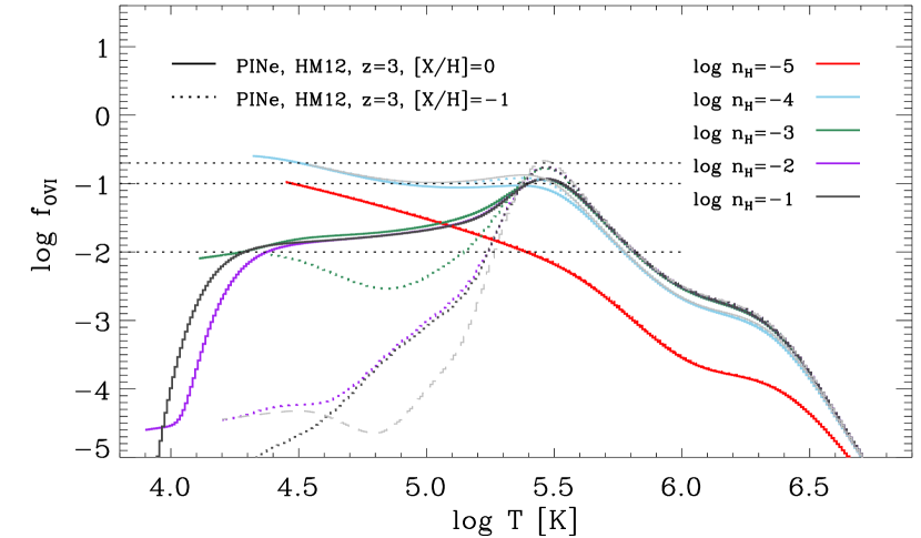
Figure 1.— Ionization fraction of O VI as a function of the temperature in an isochoric, radiatively cooling diffuse gas in the presence of a Haardt & Madau (2012) extragalactic background at $z=3$ for different densities and two metallicities according to the models of Oppenheimer & Schaye (2013). The solid and dashed gray lines are CIE calculations in the presence of the same extragalactic background at $z=3$ for $\log n_{\rm H}=-4$ and $-2$, respectively (neither photoionization nor CIE is dependent on the metallicity). The horizontal dotted lines highlight some specific ionization fractions.

4.1. Ionization Constraints on the Fraction of O VI

One of the challenges in constraining the ionization fraction of O VI and other high ions is that they probe low-density gas with temperatures where their abundances peak that are significantly less stable than at higher or lower temperatures. Gas at $0.5\times 10^{5}<T<3\times 10^{5}$ K with near solar metallicities cools very rapidly since free thermal electrons are able to excite the valence electrons into the upper states of the strong resonance transitions of these same high ions. The subsequent rapid removal of energy from the gas through spontaneous photon emission cools the gas much more rapidly than it can typically recombine. Thus, low-density plasmas at these temperatures are not likely to be in a state of collisional ionization equilibrium (CIE), especially if the gas has high metallicity.

To illustrate this for the O VI, we show in Fig. 1 predictions for the ionization fraction of O VI, $f_{\rm OVI}$, made from recent CIE and isochoric radiative cooling models by Oppenheimer & Schaye (2013) (and see also Gnat & Sternberg, 2007; Vasiliev, 2011), where the gas is also exposed to photoionization by the EUVB radiation calculated for different gas densities with a solar and tenth solar metallicity. The CIE and non-equilibrium ionization (NEI) fraction of O VI peaks around $f_{\rm OVI}\simeq 0.2$ and $0.1$, respectively, at $T_{p}\simeq 3\times 10^{5}$ K (for N V, C IV, and Si IV, the peak abundance temperatures are $2\times 10^{5}$, $10^{5}$, $0.7\times 10^{5}$ K, respectively). This value provides a strict upper limit on $f_{\rm OVI}$. At very low densities, $\log n_{\rm H}\mathrel{\hbox{\hbox to0.0pt{\hbox{\lower 4.0pt\hbox{$\sim$}}\hss}\hbox{$<$}}}-5$, the O VI production is dominated by the extragalactic background, but as the density increases, collisional ionization dominates the production of O VI at $T\mathrel{\hbox{\hbox to0.0pt{\hbox{\lower 4.0pt\hbox{$\sim$}}\hss}\hbox{$>$}}}2\times 10^{5}$ K (which corresponds to $b_{\rm OVI}\mathrel{\hbox{\hbox to0.0pt{\hbox{\lower 4.0pt\hbox{$\sim$}}\hss}\hbox{$>$}}}15$ ${\rm km\,s}^{-1}$ for purely thermal broadening); at $T>10^{6}$ K, $f_{\rm OVI}<0.003$ or about 50–60 times less than its peak ionization. At $T<2\times 10^{5}$ K, photoionization by the EUVB radiation is only efficient for $\log n_{\rm H}\mathrel{\hbox{\hbox to0.0pt{\hbox{\lower 4.0pt\hbox{$\sim$}}\hss}\hbox{$<$}}}-3.5$; for higher densities ($\log n_{\rm H}<-3$ and $T\mathrel{\hbox{\hbox to0.0pt{\hbox{\lower 4.0pt\hbox{$\sim$}}\hss}\hbox{$>$}}}2\times 10^{5}$ K), the gas must be solar metallicity or above in order to have $0.01<f_{\rm OVI}<0.1$, otherwise $f_{\rm OVI}\ll 0.001$. The ionization of the O VI (and similarly for the other high ions) can therefore be well below from their peak abundances, especially if the gas is relatively high metallicity or hot.

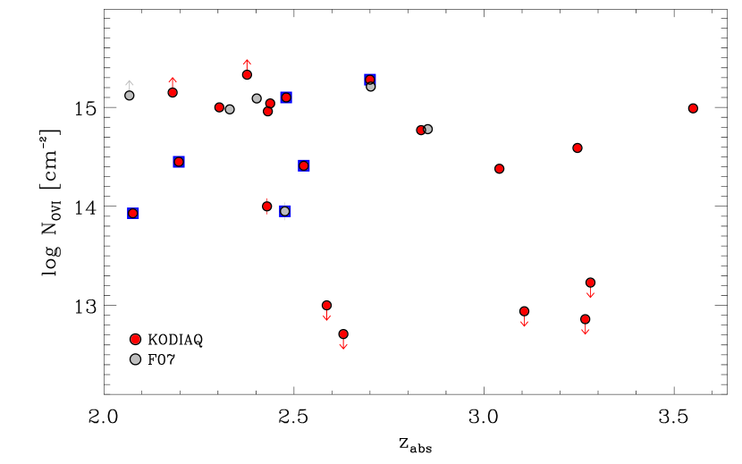
Figure 2.— Total column density of O VI associated with optical thick absorbers as a function of the redshift of the absorber. Circles with overplotted blue squares highlight the proximate systems. When the $1\sigma$ error is not apparent, it is less than the size of the circle.

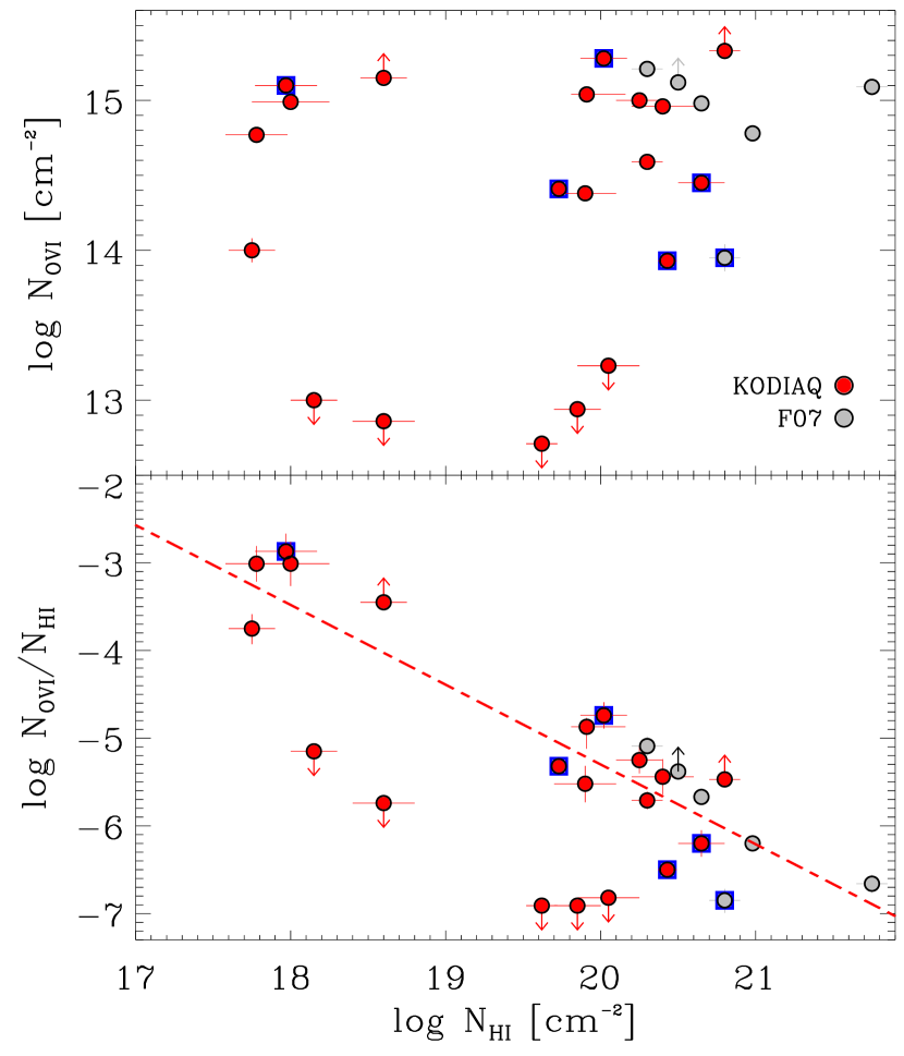
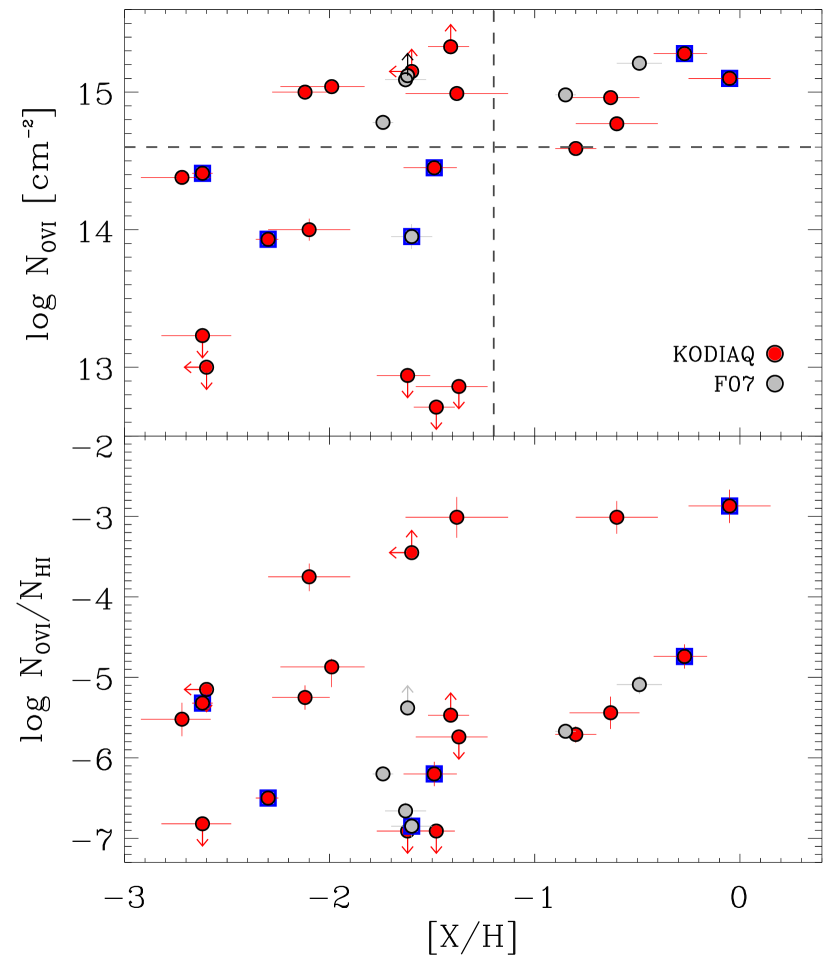
Figure 3.— Left:  Total column density of O VI and $N_{\rm OVI}$/$N_{\rm HI}$ vs. $N_{\rm HI}$. The dashed line in the bottom panel is the fit derived for O VI absorbers associated with Ly$\alpha$ forest absorbers ($\log N_{\rm HI}\mathrel{\hbox{\hbox to0.0pt{\hbox{\lower 4.0pt\hbox{$\sim$}}\hss}\hbox{$<$}}}16$) at similar redshifts from Muzahid et al. (2012). Right: Total column density of O VI and $N_{\rm OVI}$/$N_{\rm HI}$ vs. the metallicity of the cool gas. Circles with overplotted blue squares highlight the proximate systems. When the $1\sigma$ error is not apparent, it is less than the size of the circle.

4.2. General Properties from the Integrated Profiles

The detection rate of the O VI absorption in the KODIAQ sample is $15/20$ ($64$–$83$% assuming a Wilson score with a 68% confidence interval). For the LLSs, the O VI detection rate is 5/7 ($53$–$85$%), 5/8 for the SLLSs ($45$–$77$%), and 5/5 ($83$–$100\%$) for the DLAs; combining the KODIAQ and F07 samples yields a 11 detections of O VI in 11 DLAs, i.e., a detection rate $>92\%$ at the 68% confidence level. All the upper limits on $N_{\rm OVI}$ are well below the detection threshold, typically $\mathrel{\hbox{\hbox to0.0pt{\hbox{\lower 4.0pt\hbox{$\sim$}}\hss}\hbox{$<$}}}13$ dex, which is at the level or less than that observed in the local interstellar medium (Savage & Lehner, 2006). When O VI is not detected, 1) C IV is not detected either (for the absorbers where there is coverage of C IV), 2) Si IV can be present (there are 2 non-detections and 2 detections of Si IV when O VI is not detected), and 3) the velocity structure in O I and singly ionized species is simple (1 or 2 components). However, a simple velocity structure does not necessarily imply the absence of high-ion absorption (see, e.g., Fig. LABEL:f-q1243 or LABEL:f-j0831).

When O VI is detected, $\log N_{\rm OVI}$ varies from 13.93 to $>15.33$ (see Figs. 2 and 3), i.e., the O VI absorption is quite strong even though weak O VI absorbers are quite typical in O VI absorbers associated with $\log N_{\rm HI}<17$ absorbers (Simcoe et al., 2002; Muzahid et al., 2012). In fact, in the KODIAQ+F07 sample, when O VI is detected, $N_{\rm OVI}$ is remarkably large: 86% (18/21) of the absorbers have $\log N_{\rm OVI}\mathrel{\hbox{\hbox to0.0pt{\hbox{\lower 4.0pt\hbox{$\sim$}}\hss}\hbox{$>$}}}14.4$, 65% (13/21) have $\log N_{\rm OVI}\mathrel{\hbox{\hbox to0.0pt{\hbox{\lower 4.0pt\hbox{$\sim$}}\hss}\hbox{$>$}}}14.8$, and on average $\langle N_{\rm OVI}\rangle=10^{14.9\pm 0.3}$ cm${}^{-2}$. There is no apparent difference in the total column density of O VI between the proximate and intervening absorber samples as displayed in Fig. 2.

In the KODIAQ sample, the reason for the large total O VI column densities is that the O VI profiles typically extend over $200$ ${\rm km\,s}^{-1}$: we compare the full-widths, $\Delta v$, of the O VI, Si IV, and C IV profiles in Fig. 4. The average and dispersion of $\Delta v$ for O VI, C IV, and Si IV are $299\pm 90$, $269\pm 104$, and $225\pm 121$ ${\rm km\,s}^{-1}$, respectively. Except for two data points (excluding the two where O VI is partially contaminated), $\Delta v_{\rm OVI}>\Delta v_{\rm CIV}$, while for C IV and Si IV, about half the sample has $\Delta v_{\rm SiIV}\simeq\Delta v_{\rm CIV}$ and the other half $\Delta v_{\rm SiIV}<\Delta v_{\rm CIV}$. This is again quite different from the results of O VI absorbers not selected for strong H I where the line-spreads of O VI are smaller with a median of 66 ${\rm km\,s}^{-1}$ (with typically $\Delta v\mathrel{\hbox{\hbox to0.0pt{\hbox{\lower 4.0pt\hbox{$\sim$}}\hss}\hbox{$<$}}}100$–$150$ ${\rm km\,s}^{-1}$) and $\Delta v_{\rm OVI}\sim\Delta v_{\rm CIV}$ (Muzahid et al., 2012). However, the O VI properties in the KODIAQ sample are quite similar to those derived from the stacked DLA SDSS spectrum at $z\sim 2.9$ ( $N_{\rm OVI}\simeq 10^{14.6}$ cm${}^{-2}$ and $\Delta v_{\rm OVI}>\Delta v_{\rm CIV}>\Delta v_{\rm SiIV}$, see Rahmani et al., 2010, and also Fumagalli et al. 2013 who show strong O VI absorption in the composite spectrum of 38 $\tau\geq 2$ LLSs).

In the local universe, O VI absorption with $\log N_{\rm OVI}\mathrel{\hbox{\hbox to0.0pt{\hbox{\lower 4.0pt\hbox{$\sim$}}\hss}\hbox{$>$}}}14.4$ is only observed in the SMC or starburst galaxies, and with $\log N_{\rm OVI}\mathrel{\hbox{\hbox to0.0pt{\hbox{\lower 4.0pt\hbox{$\sim$}}\hss}\hbox{$>$}}}14.8$ only in starburst galaxies (Heckman et al., 2002; Grimes et al., 2009). The strength of the O VI absorption in the halos of galaxies and its relation with the level of star formation in the galaxies is demonstrated by Tumlinson et al. (2011) who found at $z<0.5$ that the dichotomy between star-forming and passive galaxies strongly affect the O VI column density in their CGM within at least 150 kpc: star-forming galaxies have typically $\log N_{\rm OVI}\mathrel{\hbox{\hbox to0.0pt{\hbox{\lower 4.0pt\hbox{$\sim$}}\hss}\hbox{$>$}}}14.5$ while more passive galaxies have $\log N_{\rm OVI}\ll 14.5$ in their CGM. The total velocity interval where high-ion absorption is observed is also similar to the breadths of the O VI profiles observed in local starburst galaxies (Heckman et al., 2001; Grimes et al., 2009) despite the different geometries. The large O VI velocity breadths and column densities therefore strongly suggest that the O VI absorption associated with $\tau_{\rm LL}>1$ absorbers at $z>2$ is strongly linked to star-forming galaxies.

There is no trend between the amount of O VI and the redshift or $N_{\rm HI}$ as displayed in Figs. 2 and 3. The strong anti-correlation between $N_{\rm OVI}$/$N_{\rm HI}$  and $N_{\rm HI}$ confirms that $N_{\rm OVI}$ and $N_{\rm HI}$ are not correlated. This anti-correlation extends with a similar slope to the Ly$\alpha$ forest at similar redshifts (see Muzahid et al., 2012, and see dashed line in the bottom left panel of Fig. 3).

On the right-hand side of Fig. 3, we show $N_{\rm OVI}$ and $N_{\rm OVI}$/$N_{\rm HI}$ as a function of the metallicity [X/H] of the cool gas. There is no evidence for a relation between $N_{\rm OVI}$/$N_{\rm HI}$ and [X/H]. There is a moderate correlation between $N_{\rm OVI}$ and [X/H] according to the rank Spearman test ($r=0.5$) significant at the 97% level for the KODIAQ+F07 excluding the upper limits. However, what seems more remarkable is the apparent division at $[{\rm X/H}]=-1.2$: For $[{\rm X/H}]\mathrel{\hbox{\hbox to0.0pt{\hbox{\lower 4.0pt\hbox{$\sim$}}\hss}\hbox{$<$}}}-1.2$, a large scatter in $N_{\rm OVI}$ is observed (spanning a factor $>100$ from $\log N_{\rm OVI}<13$ and $\log N_{\rm OVI}>15.4$), while for $[{\rm X/H}]\mathrel{\hbox{\hbox to0.0pt{\hbox{\lower 4.0pt\hbox{$\sim$}}\hss}\hbox{$>$}}}-1.2$, there are only strong O VI absorbers with $14.7\mathrel{\hbox{\hbox to0.0pt{\hbox{\lower 4.0pt\hbox{$\sim$}}\hss}\hbox{$<$}}}\log N_{\rm OVI}\mathrel{\hbox{\hbox to0.0pt{\hbox{\lower 4.0pt\hbox{$\sim$}}\hss}\hbox{$<$}}}15.3$. If our interpretation above is correct, high-$z$ metal-enriched galaxies are actively forming massive stars, enriching their CGM with large quantity of O VI (and hence metals).

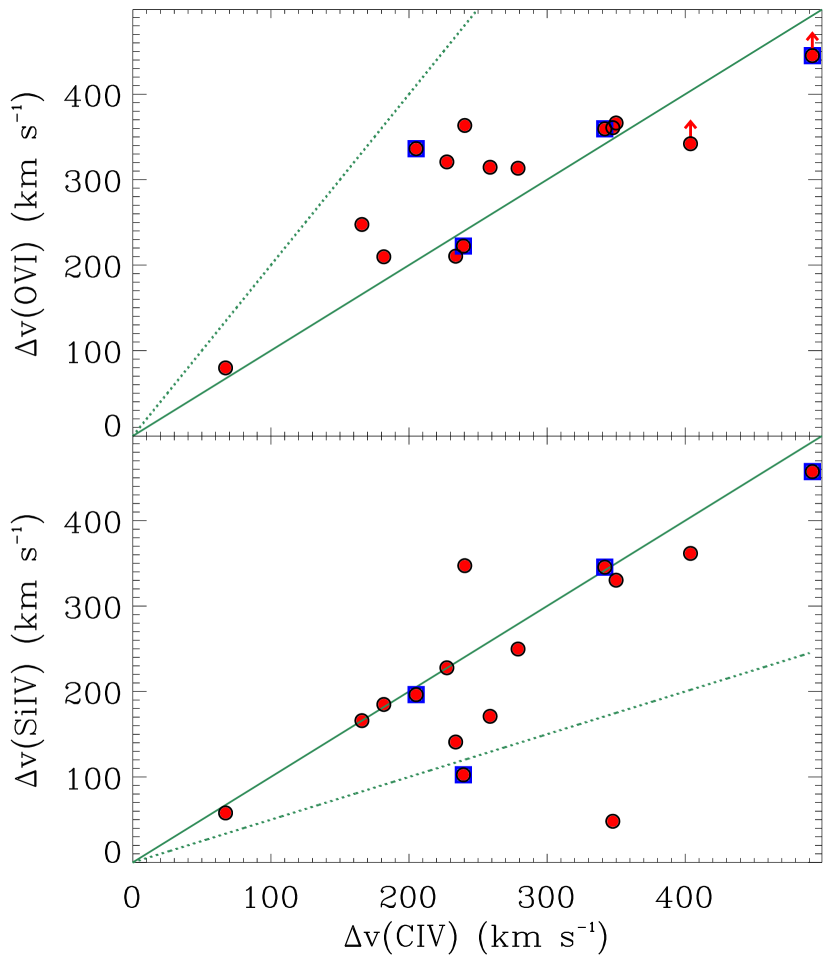
Figure 4.— Full-width comparison of the high ions. The solid green line shows a 1:1 relationship, while the dotted line is a 2:1, 1:2 relationship in the top and bottom panels, respectively. A data point with an up arrow highlight an absorber where the O VI profile is contaminated at one of the edges where C IV absorption is observed. The circles with overplotted blue squares highlight the proximate systems.

4.3. General Properties from the Velocity Profiles

The typically large velocity breadth and column density of O VI suggests that the O VI absorbers associated with $\tau_{\rm LL}>1$ absorbers at $z>2$ are tracing large-scale feedback of active star-forming galaxies. We want now to determine if there is any relationship between O VI with the other high ions and singly ionized species and how the kinematic profiles compare between the high ions. As we selected our sample based on the small contamination level of the O VI absorption by the Ly$\alpha$ and Ly$\beta$ forests and the spectral resolution is the same for all the ions for a given absorber, we can directly compare the Si IV, C IV, and O VI profiles to assess for broad similarities or dissimilarities.

We first consider four absorbers that highlight some of the overall similarities and differences between the high-ion profiles:

- Absorber $z=2.42903$ toward Q1009+2956 (see Figs. LABEL:f-q1009 and LABEL:f-fitq1009):  C IV and Si IV have both narrow and broad components and very similar component structures. A similar velocity structure is observed in the singly ionized species except for the component at $-167$ ${\rm km\,s}^{-1}$, which is only observed in C IV and Si IV. On the other hand, the O VI profiles differ entirely from all the other ions: the overall O VI profile is smoother, in particular where the main absorption is observed in C IV and Si IV between $-80$ and $+80$ ${\rm km\,s}^{-1}$; the O VI profile is more extended at positive velocities; and even where the narrow O VI absorption is observed at $-71$ ${\rm km\,s}^{-1}$, there is surprisingly no corresponding absorption in C IV and Si IV. Hence the bulk of C IV and Si IV as well as the singly ionized species trace gas that is kinematically related. Our Cloudy simulations (see §3.3) show that Si IV and Si II can be produced by photoionization by the EUVB radiation, but falls short to produce enough C IV by a factor 4. Some other ionization sources may include a harder ionizing source (e.g., from the interface of a hot gas; see Knauth et al., 2003; Borkowski et al., 1990), or photoionization of a very low density gas (Oppenheimer & Schaye, 2013), or possibly turbulent mixing layers (Slavin et al., 1993; Kwak & Shelton, 2010). O VI must, however, trace a much different type of gas that is hotter ($T\mathrel{\hbox{\hbox to0.0pt{\hbox{\lower 4.0pt\hbox{$\sim$}}\hss}\hbox{$<$}}}2\times(10^{5}$–$10^{6})$ K implied from the individual $b$-values but one — the $-71$ ${\rm km\,s}^{-1}$ component has $T<3\times 10^{4}$ K) and/or much more turbulent. No N V is observed in this absorber.

-Absorber $z=2.83437$ toward J1343+5721 (see Figs. LABEL:f-j1343 and LABEL:f-fitq1009):  For this absorber, the situation is quite different with no evidence of narrow components in the high ions that align with the cooler gas. The C IV and Si IV profiles have again matching components, with the bulk of the absorption shifted by $-131$ and $-70$ ${\rm km\,s}^{-1}$ from the strongest absorbing component in the singly ionized species. However, while the velocities of the O VI and C IV profiles at $v<-50$ ${\rm km\,s}^{-1}$ overlap, the bulk of the O VI absorption is at $-28$ ${\rm km\,s}^{-1}$. In this absorber, the high ions trace gas that is hot and/or kinematically disrupted gas, but there is a large variation in the ionic ratios of O VI to C IV (or Si IV), implying changes in the physical conditions of the gas. In this case N V $\lambda$1238 is detected and free of contamination and its profile structure follows that of O VI.

- Absorber $z=3.04026$ toward HS0757+5218 (see Figs. LABEL:f-hs0757 and LABEL:f-fiths0757):  The bulk of the absorption for the low-ions and O I is between $-30$ and $+30$ ${\rm km\,s}^{-1}$, while for the high ions, it is between $-150$ and $-30$ ${\rm km\,s}^{-1}$, so again the components of the high and low ions do not align. There is again some similarity between C IV and Si IV and the profiles of these ions show a larger number of velocity components than observed in the O VI profile. However, the AOD comparison also shows that the broad O VI component is also visible in the C IV profile. So in this case, the peak optical depth of the absorption in the high ions is largely shifted from that of the low ions, but O VI and some of the C IV  trace hot and/or kinematically disrupted gas. In this case, there is no detection of N V.

- Absorber $z=2.52569$ toward Q1243+3047 (see Figs. LABEL:f-q1243 and LABEL:f-fitq1217):  All the absorbers described above are intervening, while this SLLS is a proximate absorber. The low ions probes relatively cool and very low metallicity ($0.2\%$ solar) gas (see also Kirkman et al., 2003). The bulk of the observed absorption in the high-ion profiles is again displaced by about 40 to 120 ${\rm km\,s}^{-1}$ relative to low-ion absorption. There is, however, an excellent match between the C IV and O VI (and Si IV profiles) even though there is more structure visible in the C IV and Si IV profiles. So in this case, all the high ions trace gas governed by similar physical conditions. This better match between C IV and O VI is also observed in 3/5 proximate absorbers in the KODIAQ sample. There is also an intervening absorber ($z=2.18076$ toward Q1217+499) where all the ion profiles follow each other quite well, but in this case, all the high-ion profiles (including N V) are saturated at some level (see Fig. LABEL:f-q1217).

From this description and considering the entire sample, we can draw additional properties of the highly ionized gas probed by Si IV, C IV, O VI associated with strong H I absorbers at $2<z<4$:

$\bullet$ While the high-ion absorption profiles often overlap with those of the low ions or O I, the high-ion profiles have typically a larger velocity breadth with the bulk of their absorption often offset from the low ions by several tens or hundreds of kilometers per second. This is similar to the observations of local starbursts where the kinematics of the hot gas as traced by the O VI absorption are different from that seen in the cooler gas (Grimes et al., 2009), and therefore consistent with the idea the high ions probe outflowing gas or are strongly influenced by large-scale stellar feedback.
$\bullet$ While the velocity breadths are smaller for C IV and Si IV than O VI, a larger number of individual components is found in C IV and Si IV, or stated differently, the O VI profiles are generally smoother than those of C IV and Si IV. From the profile fitting results, we estimate that on average the number of components in the C IV and Si IV profiles are about the same, but is about 1.8 times the number of O VI components. A direct consequence of this is that on average, the $b$-values of the individual components increases with the ionization potential of the high ion (see also §4.4).

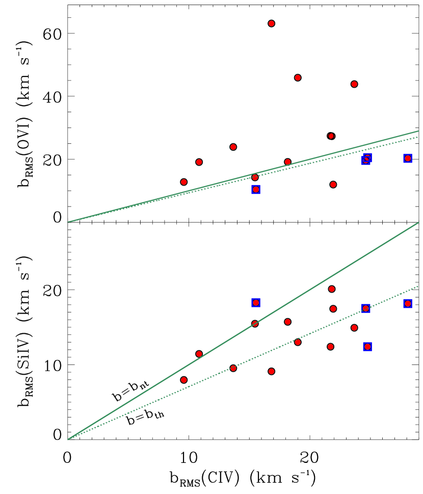
Figure 5.— Comparison of the RMS $b$-values of the high ions. $b_{\rm rms}$ is determined from the profile fit results for a given ion of a given absorber. The solid line shows a 1:1 relationship, which corresponds to the case where non-thermal motions dominate the profile broadening. The dotted line corresponds to the broadening dominated by thermal motions. The circles with overplotted blue squares highlight the proximate systems.

In Fig. 5, we compare the RMS of individual $b$-values of the high ions for each absorber: for the intervening systems, all but one absorber have $b_{\rm OVI}^{\rm rms}>b_{\rm CIV}^{\rm rms}$, while for the proximate systems $b_{\rm OVI}^{\rm rms}\leq b_{\rm CIV}^{\rm rms}$. For C IV and Si IV, there is no difference between the proximate and intervening absorbers, and for all but one absorber $b_{\rm SiIV}^{\rm rms}\mathrel{\hbox{\hbox to0.0pt{\hbox{\lower 4.0pt\hbox{$\sim$}}\hss}\hbox{$<$}}}b_{\rm CIV}^{\rm rms}$; in this case, the larger difference in the atomic weight between Si and C better separates the non-thermal and thermal broadening contributions, and since many components of C IV and Si IV are aligned it is expected that most data lie roughly between the pure-thermal and non-thermal solutions as displayed in Fig. 5 (the detailed comparison of the profiles is beyond the scope of this paper and will be made in a future KODIAQ paper).

These properties imply that the O VI absorption traces gas that is hotter and/or is more kinematically disturbed for the intervening absorbers than the gas probed by Si IV and the bulk of C IV. So even though all these ions trace highly ionized gas, O VI  often traces a different gas-phase than C IV and Si IV. The strong correlation observed here between C IV and Si IV for all the $\tau_{\rm LL}>1$ absorbers was already noted for the DLAs by Wolfe & Prochaska (2000). The absence of correlation between the velocity components between O VI and C IV (or Si IV) and the fact that the average $b$ for O VI  is quite large, typically larger than for C IV, almost certainly rule out that photoionization is a major contribution in the production of the observed O VI (see §4.4 for more details). On the other hand, for the proximate systems, there is often a much better match between the C IV and O VI profiles, implying that they may probe gas with the same physical conditions. It could also be possible that photoionization plays a major in the production of the high ions in the case that the Hubble broadening dominates the line broadening; the absorbers would then probe $\mathrel{\hbox{\hbox to0.0pt{\hbox{\lower 4.0pt\hbox{$\sim$}}\hss}\hbox{$<$}}}60$–100 kpc path length structure (see ionization models in Simcoe et al., 2002), however, as we discuss below this would be contrary to the large differences observed in the broadenings of the individual components between O VI and C IV.

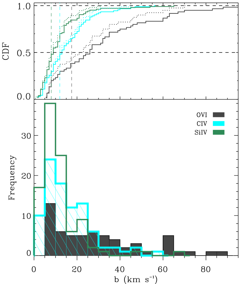
Figure 6.— Frequency and cumulative distribution functions of the $b$-value of the individual components for O VI, C IV, and Si IV  (using the results from Table LABEL:t-fit). In the bottom panel, the entire sample is used. In the top panel, the solid lines show the results for the entire sample while the dotted lines show the results for the robust sample. The vertical dashed lines in the top panel show the $b$-value corresponding at the peak-abundance temperatures for Si IV, C IV, O VI  in collisional ionization if thermal motions dominate the broadening.

4.4. Doppler Parameter

We can make a step further in characterizing the highly ionized gas by studying in more detail the individual $b$-values, which gives an upper limit on the temperature. For our analysis, it is useful to consider a cutoff on the observed Doppler parameter. Following Lehner et al. (2011), we define a $b$ cutoff, $b_{c}$, between broad and narrow components where the narrow components probe gas temperature of $7\times 10^{4}$ K in the absence of non-thermal broadening ($5\times 10^{4}$ K if we assume roughly equal thermal and non-thermal contributions to the line width). The $b_{c}$-value varies for each species such that $b_{c}=6.5$ ${\rm km\,s}^{-1}$ for Si IV, 10 ${\rm km\,s}^{-1}$ for C IV, and 9 ${\rm km\,s}^{-1}$ for O VI. In Table 4, we summarize the median, mean, dispersion of $b$, and fraction of components with $b>b_{c}$ for the various samples. In Fig. 6, we show the $b$-value distribution and cumulative distribution for O VI, C IV, and Si IV for the entire sample of absorbers. Except for a slight decrease in the mean, median, dispersion of $b$ for O VI between the robust and entire samples, there is no major difference between the various samples, and in particular between the samples that include and exclude proximate absorbers. The top panel of Fig. 6 shows the cumulative distributions for entire (solid line) and robust (dotted line) samples, demonstrating only small differences between the two samples. We therefore consider hereafter in this section the entire sample for our discussion of the Doppler parameters.

The $b$ distributions for Si IV and C IV have a prominent peak around their mean, at about 10 and 15 ${\rm km\,s}^{-1}$ ($T<2\times 10^{5}$ K), respectively, and a shallow extended wing at higher $b$. In contrast, the distribution of O VI is much flatter with about the same frequency of $b$ in each bin. Fig. 6 and Table 4 show that the mean and median of $b$ increase with the ionization energy $E_{i}$ of the ions. A similar trend is observed in the Milky Way (Lehner et al., 2011), although $\langle b\rangle$ for O VI is much larger ($\sim$40 ${\rm km\,s}^{-1}$) for the Milky Way (likely because the instrumental resolution of the Milky Way observations is much cruder, about 20 ${\rm km\,s}^{-1}$ compared to 6–8 ${\rm km\,s}^{-1}$ for the Keck HIRES spectra). Comparing our results with the high redshift study of C IV and O VI associated with the Ly$\alpha$ forest (Muzahid et al., 2012), we find a small increase in the difference of 3 ${\rm km\,s}^{-1}$ in the median $b$-values for C IV in our sample, but a significant one for O VI of 12 ${\rm km\,s}^{-1}$, implying that the O VI associated with $\tau_{\rm LL}>1$ absorbers is not produced in the same conditions or is more turbulent than in the more diffuse gas.

As it can be seen from the $b$ distributions in Fig. 6, both narrow and broad absorption components are observed in the Si IV, C IV, and O VI profiles, where the narrow components imply gas with $T<7\times 10^{4}$ K. About 20% of the O VI individual components and 30% of the Si IV and C IV components are narrow. For the O VI, this is direct evidence that the highly ionized plasma has radiatively cooled or is photoionized by the EUV and soft X-ray radiation from, e.g., cooling hot gas, or EUVB radiation. If NEI dominates the ionization of the O VI production, then the gas must be solar or higher metallicity as otherwise no significant amount of O VI would be observed at these low temperatures (see Fig. 1). We show below the $b$–$N$ correlation for O VI strongly suggests that O VI is more likely produced by collisions rather than in a gas irradiated by EUV and soft X-ray photons. We also find that 30%–40% of components of the high ions are so broad (i.e., for O VI, C IV, and Si IV, $b\geq 31,21,10$ ${\rm km\,s}^{-1}$, respectively) that they would imply ionization fraction for a given high ion $<0.003$ for any types of ionization (Oppenheimer & Schaye, 2013, and see Fig. 1) if thermal motions dominated the broadening mechanisms or if thermal and non-thermal motions contribute similar amounts of broadening. We note a large bulk flow driven by the Hubble expansion is unlikely to be a dominant broadening mechanism because there is so little correspondence between the high ion profiles; a better match between the centroid velocities and $b$-values would be expected if the Hubble flow was important.

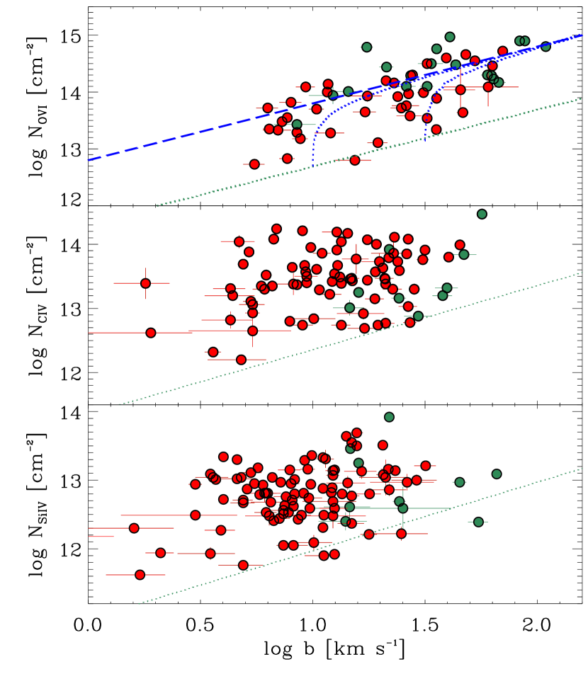
Figure 7.— Column density against the $b$-value for each individual component of O VI, C IV, and Si IV for the KODIAQ sample (using the results from Table LABEL:t-fit). Red data are more robust estimates than green data (flag ‘0’ and ‘$>0$’ in Table LABEL:t-fit, respectively). The dotted line in each panel shows $N$ vs. $b$ for a Gaussian line shape with 10% central optical depth, which represents the typical detection limit. A Spearman ranking test indicates a strong correlation between $b$ and $N$ for O VI, but not for C IV or Si IV. In the top panel, we reproduce results from Heckman et al. (2002) for reference: the curved dotted lines indicate the predictions for radiatively cooling gas for temperatures of $T_{\rm OVI}=10^{5},10^{6}$ K assuming that the cooling flow velocity is equivalent to the $b$-value; the dashed lines corresponds to the effect of blending of multiple narrow components with a velocity separation $\Delta v=0$ ${\rm km\,s}^{-1}$ (if $\Delta v\geq 10$ ${\rm km\,s}^{-1}$, then the effect would resemble to that of the radiatively cooling lines, see Heckman et al.)

In the physics of radiatively cooling or conductively heated gas, a relationship between the observed Doppler parameter and the column density is expected (Heckman et al., 2002; Edgar & Chevalier, 1986). While Heckman et al. (2002) present a heterogeneous sample of O VI measurements, several works afterwards study this relationship in more controlled environments. In the IGM at both high and low $z$, the correlation is marginal or not present (Lehner et al., 2006; Tripp et al., 2008; Muzahid et al., 2012). However, in the Milky Way disk, while Lehner et al. (2011, and see also ) show no relationship between $N$ and $b$ for C IV and Si IV, they found a strong correlation for N V and O VI. A strong correlation between $b$ and $N$ is also observed in starburst galaxies (Heckman et al., 2002; Grimes et al., 2009), which led Grimes et al. to conclude that the bulk of the O VI absorption is produced in a radiatively cooling gas produced in the interaction between the hot outflows seen in X-rays and much cooler gas seen in H$\alpha$ emission. The $b$–$N$ plot for the high ions in our sample is shown in Fig. 7. For any $b$-values within $0.5\leq\log b\leq 1.5$ (where 90% of the data lie for C IV and Si IV), $N$ for C IV and Si IV can have any values between about the maximum and minimum observed values of $N$. As noted above, for O VI, there is an overall increase in $b$ as 90% of the O VI components have $0.8\leq\log b\leq 1.9$, but over this $b$ interval, there is also correlation between $N$ and $b$. This holds for any subsamples of O VI, i.e., the entire sample, the intervening robust or entire sample. From Fig. 7, there is visually an apparent correlation for O VI, but not C IV or Si IV. This is confirmed using a ranking Spearman test: this test shows a strong correlation for the O VI intervening systems with $r=0.70$ (with a statistical significance $p\ll 0.1\%$) and for the robust intervening sample $r=0.65$ ($p\ll 0.1\%$), statistically supporting a strong correlation between $b$ and $N$ for O VI. The same result is reached if one adopts various cut offs in $N$ over all $b$-values (to account for the potential that there are different sensitivity limits as a function of $b$). In contrast, for C IV and Si IV, only a very weak correlation is observed with $r=0.2$, and at the $3\sigma$ level this relationship could happen just by chance.

The absence of strong correlation between $N$ and $b$ for C IV and Si IV and strong correlation for O VI on one hand, and the significant difference in the $b$ distribution of O VI and C IV (or Si IV) on the other hand imply that not only the gas in the LLSs, SLLSs, and DLAs is multiphase, but the bulk of the O VI may trace altogether a different type of gas, i.e., the physics that govern the O VI and the other high ions are different. The correlation between $b$ and $N$ for O VI is naturally explained by a radiatively cooling gas produced between a shock-heated outflowing gas driven possibly by massive starbursts and a cooler gas traced by singly ionized species (see Fig. 7 where we reproduced the models from Heckman et al., 2002). The scatter can be explained by various temperatures and velocities in the cooled/heated gas as well as to some photoionization by the hot plasma (Heckman et al., 2002; Knauth et al., 2003). The large scatter for C IV and Si IV suggests that photoionization by the EUVB radiation or more localized sources (stars, hot plasmas) could play an important role, as a relationship between $N$ and $b$ is not expected in that case; this is consistent with the fact that C IV and Si IV are more easily photoionized than O VI owing to their significantly smaller ionizing energy values. In §5.1, we discuss in more details the implications for the origins of the gas probed by the high ions.

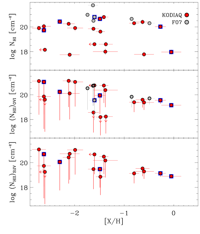
Figure 8.— The H I and H II column densities against the metallicity of the cool gas. The H II column densities are derived from O VI and Si IV assuming the ionization fractions of 0.2 and 0.4, respectively, and the metallicity of the cool photoionized gas (see §4.5 for more details). There is no relation between $N_{\rm HI}$ and the metallicity, but there is a strong anti-correlation between $N_{\rm HII}$ and the metallicity according to the rank Spearman test, which is expected since $N_{\rm HII}$ derived from a metal line is inversely proportional to the metallicity. That anti-correlation disappears when a solar metallicity in the O VI and Si IV phases is assumed and shown with the downward error bars. Circles with overplotted blue squares highlight the proximate systems.

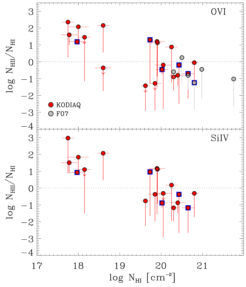
Figure 9.— Ionization-to-neutral ratio as a function of the H I column density. The filled circles are data where $N_{\rm HII}$ is derived from O VI and Si IV assuming the ionization fractions of 0.2 and 0.4, respectively, and the metallicity of the cool photoionized gas (see §4.5 for more details). The downward error bars indicate the effect of using a solar metallicity in the O VI and Si IV phases. As the highly ionized gas is not in CIE, these ionization fraction values are upper limits, so when O VI or Si IV is detected, $N_{\rm HII}$ must increase for a given metallicity. Circles with overplotted blue squares highlight the proximate systems.

4.5. Total H Column Density

In the previous sections, we have advanced several arguments that Si IV and O VI do not probe generally the same ionized gas, while C IV can be in both types of gas at various levels. To gauge the importance of the highly ionized gas relative to the neutral gas, we use Si IV and O VI to estimate the amount of H II associated with the warm highly ionized gas and hotter or more turbulent highly ionized gas, respectively. We estimate the amount of hydrogen in the ionized phase probed by O VI from $N^{\rm OVI}_{\rm HII}=N($O VI$)/(f_{\rm OVI}\,({\rm O/H}))$, where $f_{\rm OVI}=N($O VI$)/N({\rm O})$ is the ionization fraction of O VI. As we discussed in §4.1 (and see Fig. 1), the most conservative value for the ionization fraction of O VI is $f_{\rm OVI}=0.2$ (see also, e.g., Sutherland & Dopita, 1993; Gnat & Sternberg, 2007). We can similarly estimate the amount of ionized hydrogen in the Si IV-bearing gas by replacing O by Si and O VI by Si IV in the previous equation. The ionization fraction of Si IV is $f_{\rm SiIV}\leq 0.4$, and for many ionization conditions and densities, $f_{\rm SiIV}\sim 0.1$ (e.g., Oppenheimer & Schaye, 2013). As for O VI, we first adopt $f_{\rm SiIV}=0.4$ to have a lower limit on $N^{\rm SiIV}_{\rm HII}\,{\rm(Si/H)}$. In Table 5, we summarize the results from these calculations.

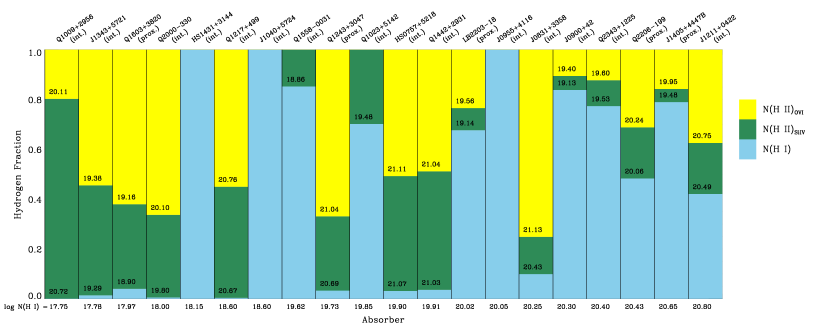
Figure 10.— Summary of the level of the hydrogen ionization and neutral breakdown in each absorber in the KODIAQ sample as a function of increasing H I column density. $N_{\rm HI}$ is directly estimated from the data (see §3.2), while $N_{\rm HII}$ is derived from O VI and Si IV assuming the ionization fractions of 0.2 and 0.4, respectively, and the metallicity of the cool photoionized gas (see §4.5 for more details). When no O VI or Si IV absorption is detected, no ionized contribution is shown. Absorbers with $18\mathrel{\hbox{\hbox to0.0pt{\hbox{\lower 4.0pt\hbox{$\sim$}}\hss}\hbox{$<$}}}\log N_{\rm HI}\ \mathrel{\hbox{\hbox to0.0pt{\hbox{\lower 4.0pt\hbox{$\sim$}}\hss}\hbox{$<$}}}20.1$ can be either predominantly ionized or neutral. For lower $N_{\rm HI}$ values, the gas is dominantly ionized, while for higher values predominantly neutral. When O VI is detected, its contribution to the ionized and often total baryon fraction is never negligible. We emphasize that neither weakly ionized gas (e.g., Al III) or hotter highly gas (e.g., O VII) is accounted for in this figure.

In both cases, the major assumptions that we have to make are that the metallicity is the same in the ionized and cool neutral gas-phases, and the metallicity is the same in each component. There is plenty of evidence in our Milky Way halo that the metallicity can change by a factor 3–10 or more between components separated by 100–200 ${\rm km\,s}^{-1}$, e.g., high-velocity clouds or tidal debris metallicity relative to the Milky Way disk metallicity (e.g., Wakker, 2001; Lehner et al., 2008a; Zech et al., 2008; Fox et al., 2013b). Prochter et al. (2010) show for one of the absorbers in the KODIAQ sample (the $z=2.43749$ absorber toward Q2000-330) a spread in metallicity between near solar to 1/100 solar, and for that sightline we take this into account. Crighton et al. (2013) also noted a factor 30 between two components of the many components observed in the KODIAQ absorber at $z=2.4379$ toward Q1442+2931. Interestingly in both cases, the strongest absorption of O VI overlaps with the velocity components with the highest metallicity estimates, while the strongest low-ion absorption tends to be in components with low metallicities, i.e., the metallicity could be systematically underestimated in the O VI-bearing gas when the metallicity of the cool gas is low. At low redshift, Savage et al. (2011a, b) directly estimated the metallicity in the cool and highly ionized gas, and found in one case (a LLS) that the highly ionized gas had more metals, and in the other case (a Ly$\alpha$ forest absorber) tentatively the opposite; in both cases, the difference in metallicity is a factor $\sim$3. Although it is too soon to draw any firm conclusion from these sparse studies, they suggest that the metallicity of the O VI-bearing gas associated with strong H I absorbers could be higher than that of the cool gas. We argued in §4.4 that some of the properties of the O VI absorbers in our sample are consistent with the idea that near solar or higher metallicities are quite likely for the O VI-bearing gas (e.g, the low $b$-values of O VI, which implies gas at temperatures far from the peak-temperature in CIE). Therefore, we also estimate $N_{\rm HII}$ assuming a solar metallicity and display both estimates in Fig. 8, which shows $N_{\rm HI}$ and $N_{\rm HII}$ as a function of the metallicity. Unsurprisingly there is no trend between $N_{\rm HI}$ and the metallicity. There is, however, an anti-correlation between $N_{\rm HII}$ estimated assuming $[{\rm X/H}]_{\rm cool}$ and the metallicity, which is not surprising either as $N_{\rm HII}\propto 1/({\rm X/H})$. That anti-correlation disappears when solar metallicity is assumed. Similar conclusions were found at low $z$ in the O VI absorbers associated with weak LLSs (Fox et al., 2013a).

At $2<z<4$, the average metallicity of the gas probed by the DLAs is around 3–12% with a very large scatter at any given $z$ (e.g., Prochaska et al., 2003; Rafelski et al., 2012), but with most values being sub-solar. So adopting a solar metallicity and the peak ionization fraction in CIE provides the most conservative estimates of $N_{\rm HII}$. In this case, the highly ionized component would only be important compared with the neutral gas column for the LLSs as displayed in Fig. 9. However, the properties of the O VI imply that the gas is in NEI (see above sections), and in this case $0.015\leq f_{\rm OVI}\leq 0.10$ for a wide range of models and temperatures, which would correspond to the high values displayed in Figs. 8 and 9 and listed in Table 5 if the solar metallicity is assumed. Similar conclusions also apply to Si IV. With that in mind, we show the magnitude of the baryon reservoir in the various forms of hydrogen as a function of increasing $N_{\rm HI}$ in Fig. 10 as reported in Table 5. The strength of the green and yellow bars relative to the blue bars clearly indicates that H I is a trace constituent for most (71%) LLSs, i.e., H II  dominates their baryon content. In the cases where high ions are detected, the total $N_{\rm H}\simeq N_{\rm HII}$ in LLSs can be as large as in the DLAs. The DLAs are on the other hand pre-dominantly neutral, but with a non-negligible amount of warm and hot and/or turbulent highly ionized gas. For the SLLSs, both naming conventions (SLLSs and sub-DLAS) can apply for these absorbers as about 60% of the SLLSs have $N_{\rm HII}\gg N_{\rm HI}$ and the other 40% $N_{\rm HII}\leq N_{\rm HI}$. Contrary to earlier assumptions, the ionization fraction can be important for any SLLSs, with low or high $N_{\rm HI}$. We also emphasize that these estimates only take into account the highly ionized gas, not the weakly warm ionized medium (WIM) probed by, e.g., Al III. Wolfe & Prochaska (2000) show indeed that Al III and singly-ionized metal line profiles are strongly correlated, but those of Al III and C IV (or Si IV) are not correlated. In the Milky Way, Lehner et al. (2011) show as well that Al III is mostly produced in the WIM, implying that Si IV and C IV have different sites of origin than does Al III. The reason for this is that most of the observed Si IV and C IV (even the narrow components) do not arise in the WIM because the WIM is strongly affected by the presence of the He I absorption edge at 24.6 eV in stellar atmosphere (Lehner et al., 2011). Therefore a photoionized phase is present and not accounted for in this paper. In §§5.2, 5.3, we discuss the implications for the baryonic and metal cosmic budgets.

5. Discussion

5.1. Origin(s) of the O VI in Intervening $\tau_{\rm LL}>1$ Absorbers: Outflows, Hot Halos, Accretion

Before discussing the implications of our findings, we remind the reader the O VI absorbers were not selected randomly. We searched specifically for LLSs, SLLSs, or DLAs for which the expected O VI absorption was not too contaminated near the velocities where H I, O I, or singly ionized species are observed. This selection ensures that the observed O VI is associated with galaxies and their CGM rather than the more diffuse IGM, and indeed the properties of the O VI in the KODIAQ sample are different from those derived in blind surveys of O VI at similar redshifts (Muzahid et al., 2012; Simcoe et al., 2002): 1) when O VI is detected, the total column and line spread of O VI are typically much larger in the KODIAQ sample than in blind O VI surveys (see §4.2), 2) there is a strong correlation between $N$ and $b$ of the individual components for O VI in the KODIAQ sample, which is not observed in blind O VI surveys at similar redshifts, and is neither observed for C IV or Si IV in any surveys (see §4.4). Although the conditions could be different at high $z$ than at low $z$, the O VI properties in the KODIAQ sample are astoundingly similar to those observed in starburst galaxies at low redshift (Grimes et al., 2009), suggesting the origin of the O VI associated with $\tau_{\rm LL}>1$ absorbers is the hot cooling gas of large-scale outflows from high redshift star-forming galaxies, possibly the Lyman break galaxies (e.g., Steidel et al., 2010). The near ubiquity of strong O VI absorption in our sample is also completely consistent with the near universal galaxy-scale outflows at $z\sim 1$–$4$ (Shapley et al., 2003; Weiner et al., 2009).

While the similarity of the O VI  properties in the KODIAQ sample and local starbursts is striking, other processes may be at play in the production of O VI. For example, any absorbers with $\log N_{\rm HI}>17$ and ${\rm[X/H]}\mathrel{\hbox{\hbox to0.0pt{\hbox{\lower 4.0pt\hbox{$\sim$}}\hss}\hbox{$<$}}}-1$ could probe cold streams according to cosmological simulations (Fumagalli et al., 2011, and see also Ribaudo et al. 2011b; Lehner et al. 2013 for low-$z$ observational results). It is also quite possible that some of the O VI traces remnants of outflows or recycled materials (e.g., Oppenheimer et al., 2010). Shen et al. (2013, hereafter S13) recently used zoom-in simulations to determine the properties of the metals (including O VI, C IV, Si IV, etc.) and H I in the CGM of massive galaxy (with a stellar mass of $1.5\times 10^{10}$ M${}_{\sun}$) at $z\sim 3$, and since the same diagnostics are investigated over similar redshifts in this simulation and our study, we primarily use these theoretical results for our discussion.

The simulated spectra along two lines of sight in S13 at impact parameters of 23 and 34 kpc show complicated structures spanning $\Delta v\sim 400$ ${\rm km\,s}^{-1}$. A qualitative comparison of the observed and simulated spectra shows that the simulated spectra have similar properties as described in §4: 1) O VI has a smoother structure than C IV and Si IV, 2) the component structures of C IV and Si IV are quite similar, but in some cases some C IV components align with O VI. In these simulations, low and high ions probe both outflows and inflows. For one of the lines of sight, some of the components also trace the CGM of a dwarf galaxy companion. Referring to Fig. 4 in S13, where the projected column density maps for the outflows and inflows are shown separately, only outflows have a large covering factor for absorbers with $\log N_{\rm OVI}\mathrel{\hbox{\hbox to0.0pt{\hbox{\lower 4.0pt\hbox{$\sim$}}\hss}\hbox{$>$}}}14.4$ at any impact parameters. Outflows and inflows have, however, similar covering factors within a virial radius of the massive galaxy for gas with $13.5\leq\log N_{\rm OVI}<14.4$. From our profile fitting analysis, 1/3 of the individual O VI components in the intervening absorbers have $\log N_{\rm OVI}\geq 14.4$ (and $\langle b\rangle=50\pm 31$ ${\rm km\,s}^{-1}$), and according to S13 simulation, these are consistent with outflows; about 1/2 have $13.5\leq\log N_{\rm OVI}<14.4$ (and $\langle b\rangle=27\pm 16$ ${\rm km\,s}^{-1}$), where both outflows and inflows could give rise to the O VI absorption. The remaining 20% of the O VI components have $\log N_{\rm OVI}\leq 13.5$ (and $\langle b\rangle=14\pm 10$ ${\rm km\,s}^{-1}$), and in the S13 model, these low O VI column densities would be produced mostly at 2–3 virial radii from a massive galaxy. According to the S13 simulations, only 1/3 of the total O VI within 2 virial radii is produced in inflows, compared to 44–50% for C IV and Si IV and 77% for H I (or singly ionized species). Therefore, similar to our conclusions above, S13 finds that O VI is mostly produced by outflows and the metallicities of the O VI gas and cool gas are not necessarily the same.

O VI absorption appears to be ubiquitous in DLAs based on the 100% detection rate in the combined KODIAQ–F07 sample, but not in LLSs and SLLSs, although the detection rate of O VI  in these absorbers is still quite high, 60–70%. For the 5 $\tau_{\rm LL}>1$ absorbers where there is no detection of O VI, the metallicity ranges between $<-2.6$ to $-1.4$ dex, which according to the simulation results from Fumagalli et al. (2011) would be likely candidates for cold streams. As O VI appears ubiquitous in the halo of $L*$ star-forming galaxies at $z\sim 0.5$ according to COS-Halos observations (Tumlinson et al., 2011) and has a near unity covering factor in massive galaxies at $z\sim 3$ according the S13 simulations, these $\tau_{\rm LL}>1$ absorbers with no associated O VI may trace cold gas inflows in the CGM of lower mass galaxies.

5.2. Cosmological Baryon Budget

At $z\sim 3$, most of the cosmic baryons ($\sim$90%) are in the diffuse IGM (Fukugita et al., 1998; Rauch et al., 1997; Weinberg et al., 1997). Adopting $\Omega_{b}=0.044$ the ratio of the total baryon density to the critical density (e.g, Spergel et al., 2003; O’Meara et al., 2001), the neutral gas of the DLAs and SLLSs contributes to about 1.8% and 0.4% of the cosmic baryons, respectively (e.g., Péroux et al., 2003, 2005; Prochaska et al., 2005, and see below). Fox et al. (2007a) show that about 1% of the baryons are in form of highly ionized gas probed by O VI in DLAs. Our present survey allows us to extend the evaluation of the cosmic baryon budget in all the $\tau_{\rm LL}>1$ absorbers and in both their neutral and highly ionized gas-phases.

As we argued in §4.3, Si IV and O VI probe largely different types of gas in the intervening absorbers, and therefore the mean gas density relative to the critical density can be obtained from the H I density distribution function ($f(N_{\rm HI})$, e.g., Tytler, 1987; Lehner et al., 2007; O’Meara et al., 2007; Prochaska et al., 2010; Ribaudo et al., 2011a), assuming that H II follows the same $f(N_{\rm HI})$ distribution:

$${\Omega_{\rm g}} = \frac{\mu_{\rm H}m_{\rm H}H_{0}}{\rho_{c}\,c}\Big{[}\int N_{\rm HI}f(N_{\rm HI})dN_{\rm HI}$$

$$+\int N_{\rm HII}^{\rm OVI}f(N_{\rm HI})dN_{\rm HI}$$

$$+\int N_{\rm HII}^{\rm SiIV}f(N_{\rm HI})dN_{\rm HI}\Big{]}$$

where $m_{\rm H}=1.673\times 10^{-24}$ g is the atomic mass of hydrogen, $\mu_{\rm H}=1.3$ corrects for the presence of helium, $\rho_{c}=3H^{2}_{0}/(8\pi G)=9.20\times 10^{-30}$ g cm${}^{-3}$ is the current critical density, and $f(N_{\rm HI})$ the column density distribution function (e.g., Tytler, 1987; Lehner et al., 2007; O’Meara et al., 2007; Prochaska et al., 2010; Ribaudo et al., 2011a). Here we use the most recent model of $f(N_{\rm HI})$ at $z=2.5$ from Prochaska et al. (2014). The first integral corresponds to the neutral gas, the second to the highly ionized gas probed by O VI, and the third to the highly ionized gas probed by Si IV. As there is no trend in $N_{\rm HII}^{\rm OVI}$ or $N_{\rm HII}^{\rm SiIV}$ with $N_{\rm HI}$ (see Fig. 10), we estimate from Table 5 the average value of $\log N_{\rm HII}$ and its dispersion for each category of absorbers. We exclude non-detections from this average, but we applied a correcting factor of 0.7 and 0.6 for the LLS and SLLS estimates, respectively, to take into account that the non-detections of O VI in these absorbers (for Si IV, the correcting factor is 0.9 for the LLLs and SLLSs). We summarize $\Omega_{\rm g}$ for each gas-phase and each $\tau_{\rm LL}>1$ absorber in Table 6; the tabulated range of values corresponds to the dispersion in $\log N_{\rm HII}$. The values for the neutral gas in SLLSs and DLAs compare well with previous results over similar redshift intervals (see above). The contribution of the neutral gas in the LLSs to the cosmological baryon budget is negligible.

The last column of Table 6 lists the contribution from these 3 gas-phases to the cosmic baryon fraction for the LLSs, SLLSs, and DLAs. The upper limit for the SLLSs suggests that the SLLSs could dominate the cosmic baryon budget for the $\tau_{\rm LL}>1$ regime. However, we note that while the average metallicities for the LLSs and DLAs are similar ( $\langle{\rm[X/H]}\rangle=-1.39$, $-1.33$, respectively ), the average SLLS metallicity is a factor 4 smaller in our KODIAQ sample ( $\langle{\rm[X/H]}\rangle=-1.93$). The average metallicity for the SLLSs in the KODIAQ sample is also about a factor 4 smaller than the average SLLS metallicity at $z\sim 2$–3 derived by Péroux et al. (2007). Hence although the very metal-poor SLLSs could hide a large amount of baryons, this result could also the subject of small number statistics. Assuming a similar average metallicity for all the $\tau_{\rm LL}>1$ absorbers, then the SLLS contribution is $0.2$–4.0%, and $\Omega_{\rm g}/\Omega_{\rm b}=3$–14% at $2<z\mathrel{\hbox{\hbox to0.0pt{\hbox{\lower 4.0pt\hbox{$\sim$}}\hss}\hbox{$<$}}}3.5$. We conclude that the highly ionized gas in the $\tau_{\rm LL}>1$ absorbers is very likely the second largest contributor after the Ly$\alpha$ forest to the baryon budget at $z\sim 2$–3. We note that if the metallicity of the O VI or Si IV gas is solar or higher (see §4.4), the contribution of the highly ionized gas in $\tau_{\rm LL}>1$ absorbers could be much smaller (a factor 10$--$20 smaller), except if this is counterbalances by much smaller ionization fraction of O VI and Si IV.

5.3. Cosmological Metal Budget

While we know where the majority of the baryons are at $z\sim 2$–3 (see §5.2), the census of metals is far more uncertain at any $z$ (e.g., Bouché et al., 2007; Peeples et al., 2014). A large fraction of the metals produced in galaxies is thought to have been expelled by $z\sim 2$ (Pettini, 2004; Bouché et al., 2005; Ferrara et al., 2005) by large-scale galaxy outflows (e.g., Shapley et al., 2003), the same outflows that we discuss in §5.1. With our KODIAQ survey, we can estimate the metal census at $z\sim 2$–3 in the neutral and highly ionized gas-phases of a sizable sample of LLSs, SLLSs, and DLAs, and hence determine if indeed a large fraction of metals are present in the CGM of galaxies at these redshifts.

The comoving metal-mass density of the $\tau_{\rm LL}>1$ absorbers could be be simply estimated using the baryon density via $\Omega_{\rm Z}=\Omega_{g}Z_{\rm abs}$ where $Z_{\rm abs}$ is the metallicity in mass units, but this approach requires we make assumptions on the ionization fraction and metallicity of the gas. A more direct strategy uses the fact that $N_{\rm OVI}$ in LLSs, SLLSs, and DLAs – when O VI is detected – does not vary much with $N_{\rm HI}$ with an average of $\langle N_{\rm OVI}\rangle=10^{14.9\pm 0.3}$ cm${}^{-2}$. This method does not require any knowledge of the metallicity and hence unlike $\Omega_{\rm g}$, the calculation of $\Omega_{\rm Z}$ does not depend on the metallicity. We can therefore directly estimate the metal budget in the $\tau_{\rm LL}>1$ absorbers in the O VI-bearing gas via,

$$\Omega_{\rm Z}^{\rm O\,VI}=\frac{\mu_{\rm O}m_{\rm O}H_{0}}{\rho_{c}\,c}\frac{\langle N_{\rm OVI}\rangle}{f_{\rm OVI}}\int f(N_{\rm HI})dN_{\rm HI},$$

where $\mu_{\rm O}=2.33$ corrects for the fact that O is 43% of the total solar metal mass, $m_{\rm O}=16m_{\rm H}$ the mass of oxygen, $f_{\rm OVI}$ the ionization fraction of O VI.

Here we choose $f_{\rm OVI}=0.1$ as a more representative of the O VI ionization fraction since the O VI gas is very likely in NEI (see §4) and since the conditions near the peak abundance of O VI are mostly transient (Gnat & Sternberg, 2007; Oppenheimer & Schaye, 2013, and below). Taking into account that 71% of the LLSs and 63% of the SLLSs have a detection of O VI, and integrating the previous equation over the various $N_{\rm HI}$ limits of the LLSs, SLLSs, DLAs, we can estimate $\Omega_{\rm Z}^{\rm OVI}$ for the LLSs, SLLSs, and DLAs. We summarize the results in Table LABEL:t-omega; the tabulated range of values corresponds to the dispersion ($\pm 0.3$ dex) in $N_{\rm OVI}$.

As discussed in §4.3, there is little correspondence between the O VI and Si IV profiles in the intervening absorbers, implying that O VI and Si IV probe in general distinct gas-phases. Hence, using the same procedure for Si IV, we can estimate $\Omega_{\rm Z}^{\rm Si\,IV}$ for the LLSs, SLLSs, and DLAs, with $\langle N_{\rm SiIV}\rangle=10^{13.7\pm 0.3}$ cm${}^{-2}$, $f_{\rm SiIV}=0.1$ (see Oppenheimer & Schaye 2013 and below), $28m_{\rm H}$ for the mass of silicon, and 4.7% for the total solar metal mass of silicon. We list the results in Table LABEL:t-omega, along with the total metal-mass density, $\Omega_{\rm Z}^{\rm h}$, of the highly ionized plasma in LLSs, SLLSs, and DLAs. As for the cosmic baryon census, these estimates do not include the WIM traced by Al III, which is not produced by the same mechanisms as the highly ionized gas (Wolfe & Prochaska, 2000; Lehner et al., 2011), or the hotter gas probed by O VII and O VIII.

With our approach, $\Omega_{\rm Z}$ depends only one variable parameter, the ionization fraction of O VI and Si IV. Oppenheimer & Schaye (2013) show that the ionization fraction of Si IV is around 0.1 for a large range of temperatures and ionization conditions, but it can reach $f_{\rm SiIV}\simeq 0.4$ if the gas is in CIE and near the peak temperature or photoionized, and hence $\Omega_{\rm Z}^{\rm Si\,IV}$ in Table LABEL:t-omega could decrease by a factor 4. On the other hand, the ionization of O VI of 0.1 is quite conservative since $0.01<f_{\rm OVI}\mathrel{\hbox{\hbox to0.0pt{\hbox{\lower 4.0pt\hbox{$\sim$}}\hss}\hbox{$<$}}}0.1$ for a wide range of temperatures when the temperature is higher or lower than the peak temperatures (see Fig. 1). Hence the O VI ionization fraction could be a factor 2–5 smaller, i.e., $\Omega_{\rm Z}^{\rm O\,VI}$ in Table LABEL:t-omega would increase by a similar factor.

For comparison, the metals in the neutral gas of DLAs and SLLSs yield $\Omega_{\rm Z}^{\rm n}\simeq 1.5\times 10^{-6}$ and $0.5\times 10^{-6}$, respectively (Bouché et al., 2007, and see also Péroux et al. 2003, 2005; Kulkarni et al. 2005, 2007; Prochaska et al. 2005). Hence at least 13–38% of the metals in DLAs are in the highly ionized plasma (see also Fox et al., 2007a). The highly ionized gas probed by Si IV and O VI in the dense CGM have at least as much and up to a factor 4 more metals than in galaxies probed by the neutral gas of DLAs.

In the more diffuse ionized gas probed by the Ly$\alpha$ forest ($\log N_{\rm HI}<17$), $\langle\Omega_{\rm Z}^{\rm Ly\alpha}\rangle\simeq 4.2\times 10^{-6}$ (Bouché et al., 2007; Schaye et al., 2003; Simcoe et al., 2004; Aguirre et al., 2004; Bergeron & Herbert-Fort, 2005). The highly ionized CGM associated with LLSs and SLLSs in the KODIAQ sample could have therefore as much metals as the more diffuse metal-enriched Ly$\alpha$ forest. We note that the mean metallicity of the Ly$\alpha$ forest in these surveys is a factor 3 larger than that of the DLAs at similar redshifts, and hence the metals in the Ly$\alpha$ forest may also probe the CGM of galaxies, especially in the high end of the Ly$\alpha$ forest ($\log N_{\rm HI}>14.5$). At low $z$, several surveys have shown that metals arises preferentially in the CGM of galaxies (e.g., Prochaska et al., 2011).

As presented in the introduction, there seems to be a missing metals problem at $z\sim 2$–3 (Pettini, 2006; Bouché et al., 2006). However, as recently shown by Peeples et al. (2014), the uncertainties in the nucleosynthesis yields (which answers the question how many metals there are) are large enough to dominate this missing metals issue, which may disappear with more accurate yields. So, we just review this issue using the fiducial value of the metal density of $\Omega_{Z}^{\rm total}\simeq 3\times 10^{-5}$ at $z\sim 2$ obtained from integrating the star formation from $z=10$ to $z=2$ (see Bouché et al., 2007). With this value, we find that about $5$–$20\%$ of metals are in the dense CGM probed by the LLSs, SLLSs, and DLAs. If we include the metals in the Ly$\alpha$ forest, $19$–$34\%$ are in the highly ionized CGM phase, compared to about 5% in the neutral gas of galaxies probed by the DLAs. While the uncertainties on the metal census are large (for the absorbers studied in this work as well as for any categories of absorbers or galaxies), our findings show that a substantial fraction of these metals is found in the highly ionized CGM of galaxies at $z\sim 2$–3.

6. Summary

With our first NASA KODIAQ survey, we have undertaken an in-depth analysis of the O VI, C IV, Si IV, and N V absorption associated with 7 LLSs, 8 SLLSs, and 5 DLAs. The high quality (S/N and resolution) of the Keck spectra has allowed us to reveal a wealth of new information on the properties of the highly ionized gas in the dense regions of the CGM and galaxies at $2<z\mathrel{\hbox{\hbox to0.0pt{\hbox{\lower 4.0pt\hbox{$\sim$}}\hss}\hbox{$<$}}}3.5$. Our main results are summarized as follows.

1. For 20 absorbers with strong H I absorption and a clean O VI region, strong O VI absorption is detected in 15 cases; The O VI detection rate is 100% for the DLAs, 71% for the LLSs, and 63% for the SLLSs. Hence there is nearly ubiquitous O VI absorption in the CGM of $z\sim 2$–$3$ galaxies.

2. Narrow and broad absorption components are seen in Si IV, C IV, and O VI, where the narrow components imply gas temperatures with $T<7\times 10^{4}$ K. About 20% of the O VI individual components and 30% of the Si IV and C IV components are narrow. For the O VI, this is evidence that the highly ionized plasma has radiatively cooled or is photoionized by the EUV and soft X-ray radiation from, e.g., a cooling hot plasma. We also find that 30%–40% of components of the high ions are so broad that it would imply an ionization fraction $<0.003$ for any types of collisional ionization or photoionization models if thermal motions dominate the broadening of the profiles or if thermal and non-thermal motions contribute similar amounts of broadening.

3. For the O VI (but not for C IV and Si IV), we find a correlation between $N$ and $b$ of the individual components, which is indicative that the bulk of the O VI absorption is produced in a radiatively cooling gas rather than in a very diffuse, extended photoionized gas by the EUVB radiation.

4. The above conclusions imply that a large fraction of the observed O VI is produced via non-equilibrium ionization processes, which also implies that some of the observed O VI-bearing gas could have a high metallicity, much higher than the cooler gas probed by H I and low ions, according to NEI models.

5. When O VI is detected, the dispersion in $N_{\rm OVI}$ is much smaller than in blind O VI surveys and $N_{\rm OVI}$ is large with $\langle N_{\rm OVI}\rangle=10^{14.9\pm 0.3}$ cm${}^{-2}$. We also find that the high ions have a large-velocity breadth ($200\leq\Delta v\leq 400$ ${\rm km\,s}^{-1}$ for O VI), where the bulk of the absorption is often displaced by several tens to a couple hundreds of kilometers per second from the cooler gas. The strength and breadth of these O VI absorbers are quite similar to those seen in low redshift starburst galaxies, which strongly suggest that the strong O VI absorbers associated with $\tau_{\rm LL}>1$ absorbers probe gas associated with the outflows of star-forming galaxies at $z\sim 2$–3.

6. The comparison with recent cosmological simulations (S13) supports the conclusion that the majority ($\sim$70%) of the O VI is produced by outflows of galaxies (independent of their mass) at $z\sim 3$. The bulk of the cooler gas (H I, C II, Si II) in these simulations traces inflows, and therefore the metallicity of the major part of the absorption of O VI and singly ionized or atomic species may not be the same as we independently argue in this work. The properties of the absorbers with no detection of O VI make them especially good candidates for cold stream inflows in dwarf galaxies; for the absorbers with O VI, inflows may also occur, but are dominated by cooler gas traced by H I and singly ionized species according to S13 simulations.

7. When the highly ionized gas is taken into account, we show that the $\tau_{\rm LL}>1$ absorbers could have as much as $3$–$14\%$ of the cosmic baryon budget at $z\sim 2$–3. Hence, almost all the baryons at $z\sim 2$–3 are found in ionized gas outside galaxies.

8. We conservatively show that $5$–$20\%$ of the metals ever produced at $2<z\mathrel{\hbox{\hbox to0.0pt{\hbox{\lower 4.0pt\hbox{$\sim$}}\hss}\hbox{$<$}}}3.5$ are in form of highly ionized metals in the circumgalactic gas of galaxies. Combined with estimates of the metal reservoir in the Ly$\alpha$ forest at similar redshifts, $19$–$34\%$ of the metals are in form of ionized gas outside galaxies, and hence a substantial fraction of metals have already been ejected by galaxy-scale outflows in the CGM at $z\sim 2$–3.

Table 1Data Sample Summary

Quasar	RA	DEC	PI	$R$	S/N	$z_{\rm{em}}$	$z_{\rm{abs}}$	$\delta v$
	(J2000)	(J2000)		(   $\times 10^{3}$)				($10^{3}$ ${\rm km\,s}^{-1}$)
Q1009+2956	10:11:55.60	$+$29:41:41.6	Sargent	48	37	2.652	2.42901	19.5
J1343+5721	13:43:29.00	$+$57:21:47.9	Prochaska	48	10	3.034	2.83437	15.6
Q1603+3820	16:04:55.40	$+$38:12:00.7	Sargent	48	54	2.510	2.47958	2.6
Q2000-330	20:03:24.12	$-$32:51:45.0	Cowie	72	7	3.783	3.54996	15.4
HS1431+3144	14:33:16.10	$+$31:31:26.3	Prochaska	36	29	2.940	2.58615	29.6
Q1217-499	12:19:30.88	$+$49:40:54.3	Pettini	48	10	2.633	2.18076	42.6
J1040+5724	10:40:18.52	$+$57:24:48.1	Prochaska	36	13	3.426	3.26620	11.2
Q1558-0031	15:58:10.16	$-$00:31:20.0	Prochaska	36	20	2.827	2.62999	16.3
Q1243+3047	12:46:10.90	$+$30:31:31.0	Prochaska	48	9	2.560	2.52569	2.9
Q1023+5142	10:23:25.25	$+$51:42:50.8	Hamann	48	9	3.447	3.10586	24.9
HS0757+5218	08:01:17.80	$+$04:22:23.9	Cowie	36	6	3.235	2.37654	14.4
Q1442+2931	14:42:44.52	$+$29:31:45.3	Sargent	48	34	2.638	2.43749	17.4
LB2203-18	22:06:39.61	$-$18:18:46.3	Prochaska	48	14	2.728	2.69985	2.4
J0955+4116	09:55:41.94	$+$41:16:53.9	Pettini	36	7	3.420	3.27987	9.8
J0831+3358	08:31:02.57	$+$33:58:02.5	Pettini	36	10	2.429	2.30361	11.4
J0900+42	09:00:32.9	$+$42:15:45.0	Prochaska	48	21	3.290	3.24571	3.2
Q2343+1225	23:46:28.32	$+$12:48:59.1	Steidel	48	31	2.763	2.43125	29.0
Q2206-199	22:08:52.22	$-$19:43:57.0	Steidel	36	11	2.559	2.07617	47.1
J1405+4447B	14:05:01.47	$+$44:47:56.5	Ellison, Martin	36	9	2.218	2.19707	2.0
J1211+0422	12:11:17.65	$+$52:10:34.6	Prochaska	48	12	2.526	2.37654	43.8

Table 2Total Column Densities

Quasar	$z_{\rm{abs}}$	$\log N_{\rm HI}$	$\log N_{\rm SiII}$	$\log N_{\rm OVI}$	$\log N_{\rm NV}$	$\log N_{\rm CIV}$	$\log N_{\rm SiIV}$
Q1009+2956	2.42901	$17.75\pm 0.15$	$12.72\pm 0.03$	$14.00\pm 0.08$	$<12.3$	$13.92\pm 0.01$	$13.73\pm 0.01$
J1343+5721	2.83437	$17.78\pm 0.20$	$13.45\pm 0.03$	$14.77\pm 0.03$	$\leq 14.06\pm 0.02$	$14.22\pm 0.03$	$13.80\pm 0.04$
Q1603+3820	2.47958	$17.97\pm 0.20$	$14.27\pm 0.05$	$15.10\pm 0.05$	$14.08\pm 0.01$	$14.98\pm 0.01$	$13.96\pm 0.01$
Q2000-330	3.54996	$18.00\pm 0.25$	$13.24\pm 0.02$	$14.99\pm 0.03$	$\cdots$	$14.31\pm 0.02$	$13.91\pm 0.02$
HS1431+3144	2.58615	$18.15\pm 0.15$	$12.19\pm 0.13$	$<13.0$	$\cdots$	$<12.2$	$<11.8$
Q1217-499	2.18076	$18.60\pm 0.15$	$13.67\pm 0.01$	$>15.15$	$>15.18$	$>15.07$	$14.18\pm 0.04$
J1040+5724	3.26620	$18.60\pm 0.20$	$13.32\pm 0.05$	$<12.9$	$<12.9$	$\cdots$	$\cdots$
Q1558-0031	2.62999	$19.62\pm 0.10$	$13.53\pm 0.02$	$<12.7$	$\cdots$	$<12.6$	$12.49\pm 0.03$
Q1243+3047	2.52569	$19.73\pm 0.04$	$13.10\pm 0.05$	$14.41\pm 0.02$	$<12.6$	$13.64\pm 0.02$	$13.18\pm 0.02$
Q1023+5142	3.10586	$19.85\pm 0.15$	$13.59\pm 0.01$	$<13.2$	$<13.1$	$13.48\pm 0.08$	$12.97\pm 0.02$
HS0757+521	3.04026	$19.90\pm 0.20$	$13.01\pm 0.01$	$14.38\pm 0.05$	$13.09\pm 0.10$	$13.98\pm 0.01$	$13.46\pm 0.02$
Q1442+2931	2.43749	$19.91\,^{+0.10}_{-0.25}$	$13.92\pm 0.01$	$15.04\pm 0.01$	$\cdots$	$>14.9$	$14.15\pm 0.02$
LB2203-18	2.69985	$20.02\pm 0.15$	$14.58\pm 0.04$	$15.28\pm 0.01$	$<12.9$	$14.54\pm 0.01$	$13.98\pm 0.01$
J0955+4116	3.27987	$20.05\pm 0.20$	$12.74\pm 0.04$	$<13.2$	$<13.0$	$<12.6$	$<12.2$
J0831+3358	2.30361	$20.25\pm 0.15$	$13.71\pm 0.04$	$15.00\pm 0.02$	$\leq 13.59$	$14.33\pm 0.02$	$13.42\pm 0.02$
J0900+42	3.24571	$20.30\pm 0.10$	$>14.95$	$14.59\pm 0.01$	$12.59\pm 0.14$	$13.65\pm 0.02$	$13.44\pm 0.01$
Q2343+1225	2.43125	$20.40\pm 0.20$	$>15.06$	$14.96\pm 0.01$	$\cdots$	$14.70\pm 0.01$	$14.01\pm 0.01$
Q2206-199	2.07617	$20.43\pm 0.06$	$13.64\pm 0.01$	$13.93\pm 0.05$	$<12.2$	$13.75\pm 0.01$	$12.87\pm 0.02$
J1405+4447B	2.19707	$20.65\pm 0.15$	$14.85\pm 0.05$	$14.45\pm 0.02$	$13.21\pm 0.08$	$13.83\pm 0.03$	$13.10\pm 0.04$
J1211+0422	2.37654	$20.80\pm 0.10$	$14.91\pm 0.04$	$>15.33$	$13.64\pm 0.02$	$>14.92$	$14.19\pm 0.01$

Note. — Detailed descriptions and uncertainties (blending, continuum, etc.) on the column densities are discussed in §§3.1 and 3.2 and in the appendix. The “$>$” symbol means that the weakest available line is saturated. The “$<$” symbol implies that a given species has not been detected and the reported value is a $3\sigma$ estimate. The “$\leq$” implies that the profile may be contaminated. Absence of value implies that the lines are contaminated for N V and not observed for C IV and Si IV.

Table 3Metallicity of the Cool Gas Phase

Quasar	$z_{\rm{abs}}$	$\log N_{\rm HI}$	$\log N_{X}$	$\log({\rm X/H})_{\sun}$	$[{\rm X/H}]$	$[{\rm X/H}]_{\rm adopt}$
Q1009+2956	$2.42901$	$17.75\pm 0.15$	$<12.02$	$-3.31$	$<-2.42$	$-2.10\pm 0.20$
J1343+5721	$2.83437$	$17.78\pm 0.20$	$13.82\pm 0.02$	$-3.31$	$-0.65\,^{+0.14}_{-0.20}$	$-0.60\pm 0.20$
Q1603+3820	$2.47958$	$17.97\pm 0.20$	$14.66\pm 0.02$	$-3.31$	$0.00\,^{+0.14}_{-0.20}$	$-0.05\pm 0.20$
Q2000-330	$3.54996$	$18.00\pm 0.25$	$13.31\pm 0.04$	$-3.31$	$-1.38\,^{+0.16}_{-0.26}$	$-1.35\pm 0.25$
HS1431+3144	$2.58615$	$18.15\pm 0.15$	$<12.24$	$-3.31$	$<-2.60$	$<-2.60$
Q1217-499	$2.18076$	$18.60\pm 0.15$	$<13.79$	$-3.31$	$<-1.50$	$-1.60:$
J1040+5724	$3.26620$	$18.60\pm 0.20$	$13.92\pm 0.03$	$-3.31$	$-1.37\,^{+0.14}_{-0.21}$	$-1.37\,^{+0.14}_{-0.21}$
Q1558-0031	$2.62999$	$19.62\pm 0.10$	$14.83\pm 0.04$	$-3.31$	$-1.48\,^{+0.09}_{-0.11}$	$-1.48\,^{+0.09}_{-0.11}$
Q1243+3047	$2.52569$	$19.73\pm 0.04$	$13.80\pm 0.03$	$-3.31$	$-2.62\pm 0.05$	$-2.62\pm 0.05$
Q1023+5142	$3.10586$	$19.85\pm 0.15$	$14.92\pm 0.03$	$-3.31$	$-1.72\,^{+0.11}_{-0.21}$	$-1.62\,^{+0.11}_{-0.15}$
HS0757+521	$3.04026$	$19.90\pm 0.20$	$13.87\pm 0.02$	$-3.31$	$-2.72\,^{+0.14}_{-0.20}$	$-2.72\,^{+0.14}_{-0.20}$
Q1442+2931	$2.43749$	$19.91\,^{+0.10}_{-0.25}$	$14.61\pm 0.01$	$-3.31$	$-1.99\,^{+0.16}_{-0.25}$	$-1.99\,^{+0.16}_{-0.25}$
LB2203-18	$2.69985$	$20.02\pm 0.15$	$14.89\pm 0.02$	$-4.86$	$-0.27\,^{+0.11}_{-0.15}$	$-0.27\,^{+0.11}_{-0.15}$
J0955+4116	$3.27987$	$20.05\pm 0.20$	$14.12\pm 0.04$	$-3.31$	$-2.62\,^{+0.14}_{-0.21}$	$-2.62\,^{+0.14}_{-0.21}$
J0831+3358	$2.30361$	$20.25\pm 0.15$	$14.82\pm 0.05$	$-3.31$	$-2.12\,^{+0.12}_{-0.16}$	$-2.12\,^{+0.12}_{-0.16}$
J0900+42	$3.24571$	$20.30\pm 0.10$	$14.64\pm 0.02$	$-4.86$	$-0.80\,^{+0.08}_{-0.10}$	$-0.80\,^{+0.08}_{-0.10}$
Q2343+1225	$2.43125$	$20.40\pm 0.20$	$14.91\pm 0.03$	$-4.86$	$-0.63\,^{+0.14}_{-0.20}$	$-0.63\,^{+0.14}_{-0.20}$
Q2206-199	$2.07617$	$20.43\pm 0.06$	$13.64\pm 0.01$	$-4.49$	$-2.30\,^{+0.05}_{-0.06}$	$-2.30\,^{+0.05}_{-0.06}$
J1405+4447	$2.19707$	$20.65\pm 0.15$	$14.30\pm 0.03$	$-4.86$	$-1.49\,^{+0.11}_{-0.15}$	$-1.49\,^{+0.11}_{-0.15}$
J1211+0422	$2.37654$	$20.80\pm 0.10$	$14.53\pm 0.04$	$-4.86$	$-1.41\,^{+0.09}_{-0.11}$	$-1.41\,^{+0.09}_{-0.11}$

Table 4Mean and Median of the Doppler Parameters and Fraction of Broad Components

Ion	m	$\langle b\rangle$	$\bar{b}$	$f(b>b_{c})$
		(${\rm km\,s}^{-1}$)	(${\rm km\,s}^{-1}$)	(%)
Entire Sample
Si IV	105	$12\pm 10$	$9$	$71\pm 5$
C IV	91	$16\pm 11$	$13$	$63\pm 5$
O VI	60	$31\pm 23$	$26$	$80\pm 5$
Robust Entire Sample
Si IV	94	$10\pm 6$	$8$	$68\pm 6$
C IV	78	$14\pm 8$	$13$	$60\pm 6$
O VI	40	$25\pm 17$	$23$	$75\pm 8$
Intervening Sample
Si IV	69	$11\pm 9$	$9$	$71\pm 6$
C IV	70	$16\pm 10$	$13$	$69\pm 6$
O VI	39	$31\pm 24$	$26$	$83\pm 6$
Robust Intervening Sample
Si IV	63	$10\pm 6$	$9$	$71\pm 6$
C IV	56	$15\pm 8$	$13$	$66\pm 7$
O VI	29	$27\pm 17$	$25$	$79\pm 9$

Note. — The $m$ value represents the size of each sample. $\langle b\rangle$ is the mean value of $b$ with its 1$\sigma$ dispersion for a given sample, while $\bar{b}$ is the median. $f(b>b_{c})$ is the fraction of components with $b>b_{c}$, the $b$-value cutoff between broad and narrow components where the narrow components probe gas temperature of about $7\times 10^{4}$ K in the absence of nonthermal broadening ( $b_{c}=6.5$ ${\rm km\,s}^{-1}$ for Si IV, 10 ${\rm km\,s}^{-1}$ for C IV, 9 ${\rm km\,s}^{-1}$ for O VI).

Table 5Neutral and Ionized Gas Column Densities

Quasar	$z_{\rm{abs}}$	$\log N_{\rm HI}$	$\log N^{\rm OVI}_{\rm HII}$	$\log N^{\rm SiIV}_{\rm HII}$	$N^{\rm OVI}_{\rm HII}/N_{\rm HI}$	$N^{\rm SiIV}_{\rm HII}/N_{\rm HI}$
Q1009+2956	$2.42901$	$17.75\pm 0.15$	$>20.1$	$>20.7$	$>228.5$	$>928.8$
J1343+5721	$2.83437$	$17.78\pm 0.20$	$>19.8$	$>19.3$	$>39.7$	$>32.2$
Q1603+3820	$2.47958$	$17.97\pm 0.20$	$>19.2$	$>18.9$	$>15.5$	$>8.5$
Q2000-330	$3.54996$	$18.00\pm 0.25$	$>20.1$	$>19.8$	$>120.2$	$>68.3$
HS1431+314	$2.58615$	$18.15\pm 0.15$	$<19.6$	$<20.5$	$<28.8$	$<217.7$
Q1217-499	$2.18076$	$18.60\pm 0.15$	$>20.8:$	$>20.7:$	$>144.2:$	$>116.9:$
J1040+5724	$3.26620$	$18.60\pm 0.20$	$<18.2$	$\cdots$	$<0.4$	$\cdots$
Q1558-0031	$2.62999$	$19.62\pm 0.10$	$<18.2$	$>18.9$	$<0.04$	$>0.2$
Q1243+3047	$2.52569$	$19.73\pm 0.04$	$>21.0$	$>20.7$	$>20.4$	$>9.1$
Q1023+5142	$3.10586$	$19.85\pm 0.15$	$<18.8$	$>19.5$	$<0.1$	$>0.4$
HS0757+5218	$3.04026$	$19.90\pm 0.20$	$>21.1$	$>21.1$	$>16.2$	$>14.7$
Q1442+2931	$2.43749$	$19.91\,^{+0.10}_{-0.25}$	$>21.0$	$>21.0$	$>13.5$	$>13.1$
LB2203-18	$2.69985$	$20.02\pm 0.15$	$>19.6$	$>19.1$	$>0.4$	$>0.1$
J0955+4116	$3.27987$	$20.05\pm 0.20$	$<19.9$	$<19.7$	$<0.6$	$<0.5$
J0831+3358	$2.30361$	$20.25\pm 0.15$	$>21.1$	$>20.4$	$>7.6$	$>1.5$
J0900+42	$3.24571$	$20.30\pm 0.10$	$>19.4$	$>19.1$	$>0.1$	$>0.1$
Q2343+1225	$2.43125$	$20.40\pm 0.20$	$>19.6$	$>19.5$	$>0.2$	$>0.1$
Q2206-199	$2.07617$	$20.43\pm 0.06$	$>20.2$	$>20.1$	$>0.6$	$>0.4$
J1405+4447	$2.19707$	$20.65\pm 0.15$	$>20.0$	$>19.5$	$>0.2$	$>0.1$
J1211+0422	$2.37654$	$20.80\pm 0.10$	$>20.8$	$>20.5$	$>0.9$	$>0.5$

Note. — See §4.5 for details on how $N_{\rm HII}$ is derived from $N_{\rm OVI}$ and $N_{\rm SiIV}$. For the cases where O VI or Si IV are not detected, we have set the ionization fraction of O VI and Si IV to 0.2 and 0.4, respectively. The colon indicates that the values are uncertain because the metallicity correction is uncertain.

Table 6Cosmic Baryonic Census of $\tau_{\rm LL}>1$ absorbers at $z\sim 2$–$3$

Absorbers	$\Omega_{\rm g}^{\rm HI}$	$\Omega_{\rm g}^{\rm HII}({\rm SiIV})$	$\Omega_{\rm g}^{\rm HII}({\rm OVI})$	$\Omega_{\rm g}/\Omega_{\rm b}$
	($10^{-3}$)	($10^{-3}$)	($10^{-3}$)	(%)
LLS	0.0077	0.04–1.9	0.08–1.2	0.4–7
SLLS	0.17	0.04–2.5	0.2–4.4	0.9–16
DLA	0.79	0.02–0.2	0.03–0.4	2–3

Note. — We define $\Omega_{\rm g}=\Omega_{\rm g}^{\rm HI}+\Omega_{\rm g}^{\rm HII}({\rm SiIV})+\Omega_{\rm g}^{\rm HII}({\rm OVI})$ and use $\Omega_{b}=0.044$ as the ratio of the total baryon density to the critical density (e.g, Spergel et al., 2003; O’Meara et al., 2001). The calculation of $\Omega_{\rm g}^{\rm HII}$ is inversely proportional to the ionization fraction of Si IV and O VI and the metallicity; we use values from Table 5 to estimate $\Omega_{\rm g}^{\rm HII}$ (see §5.2 for more details). Note that the average metallicity for the SLLSs is a factor 4 smaller than for the DLAs and LLSs in the KODIAQ sample, which drive the high value of $\Omega_{\rm g}$ for the SLLSs.

References

- Aguirre et al. (2004) Aguirre, A., Schaye, J., Kim, T.-S., et al. 2004, ApJ, 602, 38
- Asplund et al. (2009) Asplund, M., Grevesse, N., Sauval, A. J., & Scott, P. 2009, ARA&A, 47, 481
- Bergeron & Herbert-Fort (2005) Bergeron, J., & Herbert-Fort, S. 2005, IAU Colloq. 199: Probing Galaxies through Quasar Absorption Lines, 265
- Bergeron et al. (1994) Bergeron, J., Petitjean, P., Sargent, W. L. W., et al. 1994, ApJ, 436, 33
- Bird et al. (2013) Bird, S., Vogelsberger, M., Sijacki, D., et al. 2013, MNRAS, 429, 3341
- Borkowski et al. (1990) Borkowski, K. J., Balbus, S. A., & Fristrom, C. C. 1990, ApJ, 355, 501
- Bouché et al. (2007) Bouché, N., Lehnert, M. D., Aguirre, A., Péroux, C., & Bergeron, J. 2007, MNRAS, 378, 525
- Bouché et al. (2005) Bouché, N., Lehnert, M. D., & Péroux, C. 2005, MNRAS, 364, 319
- Bouché et al. (2006) Bouché, N., Lehnert, M. D., & Péroux, C. 2006, MNRAS, 367, L16
- Bowen et al. (2008) Bowen, D. V., Jenkins, E. B., Tripp, T. M., et al. 2008, ApJS, 176, 59
- Bowen et al. (2002) Bowen, D. V., Pettini, M., & Blades, J. C. 2002, ApJ, 580, 169
- Carswell et al. (2002) Carswell, B., Schaye, J., & Kim, T.-S. 2002, ApJ, 578, 43
- Chen et al. (2005) Chen, H.-W., Prochaska, J. X., Weiner, B. J., Mulchaey, J. S., & Williger, G. M. 2005, ApJ, 629, L25
- Crighton et al. (2013) Crighton, N. H. M., Hennawi, J. F., & Prochaska, J. X. 2013, ApJ, 776, L18
- Dessauges-Zavadsky et al. (2009) Dessauges-Zavadsky, M., Ellison, S. L., & Murphy, M. T. 2009, MNRAS, 396, L61
- Dickinson et al. (2003) Dickinson, M., Papovich, C., Ferguson, H. C., & Budavári, T. 2003, ApJ, 587, 25
- Edgar & Chevalier (1986) Edgar, R. J., & Chevalier, R. A. 1986, ApJ, 310, L27
- Ferland et al. (2013) Ferland, G. J., Porter, R. L., van Hoof, P. A. M., et al. 2013, Rev. Mex. de Astron. y Astr. , 49, 137
- Ferrara et al. (2005) Ferrara, A., Scannapieco, E., & Bergeron, J. 2005, ApJ, 634, L37
- Fitzpatrick & Spitzer (1997) Fitzpatrick, E. L., & Spitzer, L., Jr. 1997, ApJ, 475, 623
- Fox et al. (2013a) Fox, A. J., Lehner, N., Tumlinson, J., et al. 2013a, ApJ, 778, 187
- Fox et al. (2007a) Fox, A. J., Petitjean, P., Ledoux, C., & Srianand, R. 2007a, A&A, 465, 171 [F07]
- Fox et al. (2007c) Fox, A. J., Petitjean, P., Ledoux, C., & Srianand, R. 2007b, ApJ, 668, L15
- Fox et al. (2013b) Fox, A. J., Richter, P., Wakker, B. P., et al. 2013b, ApJ, 772, 110
- Fukugita et al. (1998) Fukugita, M., Hogan, C. J., & Peebles, P. J. E. 1998, ApJ, 503, 518
- Fumagalli et al. (2013) Fumagalli, M., O’Meara, J. M., Prochaska, J. X., & Worseck, G. 2013, ApJ, 775, 78
- Fumagalli et al. (2011) Fumagalli, M., Prochaska, J. X., Kasen, D., et al. 2011, MNRAS, 418, 1796
- Gnat & Sternberg (2007) Gnat, O., & Sternberg, A. 2007, ApJS, 168, 213
- Grimes et al. (2009) Grimes, J. P., Heckman, T., Aloisi, A., et al. 2009, ApJS, 181, 272
- Haardt & Madau (2012) Haardt, F., & Madau, P. 2012, ApJ, 746, 125
- Heckman et al. (2002) Heckman, T. M., Norman, C. A., Strickland, D. K., & Sembach, K. R. 2002, ApJ, 577, 691
- Heckman et al. (2001) Heckman, T. M., Sembach, K. R., Meurer, G. R., et al. 2001, ApJ, 554, 1021
- Herbert-Fort et al. (2006) Herbert-Fort, S., Prochaska, J. X., Dessauges-Zavadsky, M., et al. 2006, PASP, 118, 1077
- Jenkins et al. (2000) Jenkins, E. B., Oegerle, W. R., Gry, C., et al. 2000, ApJ, 538, L81
- Knauth et al. (2003) Knauth, D. C., Howk, J. C., Sembach, K. R., Lauroesch, J. T., & Meyer, D. M. 2003, ApJ, 592, 964
- Kobayashi (2004) Kobayashi, C. 2004, MNRAS, 347, 740
- Kirkman & Tytler (1997) Kirkman, D., & Tytler, D. 1997, ApJ, 489, L123
- Kirkman & Tytler (1999) Kirkman, D., & Tytler, D. 1999, ApJ, 512, L5
- Kirkman et al. (2003) Kirkman, D., Tytler, D., Suzuki, N., O’Meara, J. M., & Lubin, D. 2003, ApJS, 149, 1
- Kulkarni et al. (2005) Kulkarni, V. P., Fall, S. M., Lauroesch, J. T., et al. 2005, ApJ, 618, 68
- Kulkarni et al. (2007) Kulkarni, V. P., Khare, P., Péroux, C., et al. 2007, ApJ, 661, 88
- Kwak & Shelton (2010) Kwak, K., & Shelton, R. L. 2010, ApJ, 719, 523
- Lanzetta et al. (1995) Lanzetta, K. M., Bowen, D. V., Tytler, D., & Webb, J. K. 1995, ApJ, 442, 538
- Lehner et al. (2008a) Lehner, N., Howk, J. C., Keenan, F. P., & Smoker, J. V. 2008a, ApJ, 678, 219
- Lehner et al. (2008b) Lehner, N., Howk, J. C., Prochaska, J. X., & Wolfe, A. M. 2008b, MNRAS, 390, 2
- Lehner et al. (2013) Lehner, N., Howk, J. C., Tripp, T. M., et al. 2013, ApJ, 770, 138
- Lehner et al. (2003) Lehner, N., Jenkins, E. B., Gry, C., et al. 2003, ApJ, 595, 858
- Lehner et al. (2009) Lehner, N., Prochaska, J. X., Kobulnicky, H. A., et al. 2009, ApJ, 694, 734
- Lehner et al. (2007) Lehner, N., Savage, B. D., Richter, P., et al. 2007, ApJ, 658, 680
- Lehner et al. (2006) Lehner, N., Savage, B. D., Wakker, B. P., Sembach, K. R., & Tripp, T. M. 2006, ApJS, 164, 1
- Lehner et al. (2011) Lehner, N., Zech, W. F., Howk, J. C., & Savage, B. D. 2011, ApJ, 727, 46
- Lu et al. (1998) Lu, L., Sargent, W. L. W., & Barlow, T. A. 1998, AJ, 115, 55
- Lu & Savage (1993) Lu, L., & Savage, B. D. 1993, ApJ, 403, 127
- Madau et al. (1996) Madau, P., Ferguson, H. C., Dickinson, M. E., et al. 1996, MNRAS, 283, 1388
- Misawa et al. (2007) Misawa, T., Tytler, D., Iye, M., et al. 2007, AJ, 134, 1634
- Morton (2003) Morton, D. C. 2003, ApJS, 149, 205
- Morris & Jannuzi (2006) Morris, S. L., & Jannuzi, B. T. 2006, MNRAS, 367, 1261
- Morris et al. (1991) Morris, S. L., Weymann, R. J., Savage, B. D., & Gilliland, R. L. 1991, ApJ, 377, L21
- Muzahid et al. (2012) Muzahid, S., Srianand, R., Bergeron, J., & Petitjean, P. 2012, MNRAS, 421, 446
- O’Meara et al. (2006) O’Meara, J. M., Burles, S., Prochaska, J. X., et al. 2006, ApJ, 649, L61
- O’Meara et al. (2007) O’Meara, J. M., Prochaska, J. X., Burles, S., et al. 2007, ApJ, 656, 666
- O’Meara et al. (2001) O’Meara, J. M., Tytler, D., Kirkman, D., et al. 2001, ApJ, 552, 718
- Oppenheimer et al. (2010) Oppenheimer, B. D., Davé, R., Kereš, D., et al. 2010, MNRAS, 406, 2325
- Oppenheimer & Schaye (2013) Oppenheimer, B. D., & Schaye, J. 2013, MNRAS, 434, 1043
- Pagel (2002) Pagel, B. E. J. 2002, Chemical Enrichment of Intracluster and Intergalactic Medium, ASP Conference Proceedings, Ed. Roberto Fusco-Femiano and Francesca Matteucci, 253, 489
- Peeples et al. (2014) Peeples, M. S., Werk, J. K., Tumlinson, J., et al. 2014, ApJ, in press, [arXiv:1310.2253]
- Penton et al. (2002) Penton, S. V., Stocke, J. T., & Shull, J. M. 2002, ApJ, 565, 720
- Péroux et al. (2006) Péroux, C., Meiring, J. D., Kulkarni, V. P., et al. 2006, MNRAS, 372, 369
- Péroux et al. (2005) Péroux, C., Dessauges-Zavadsky, M., D’Odorico, S., Sun Kim, T., & McMahon, R. G. 2005, MNRAS, 363, 479
- Péroux et al. (2007) Péroux, C., Dessauges-Zavadsky, M., D’Odorico, S., Sun Kim, T., & McMahon, R. G. 2007, MNRAS, 382, 177
- Péroux et al. (2003) Péroux, C., McMahon, R. G., Storrie-Lombardi, L. J., & Irwin, M. J. 2003, MNRAS, 346, 1103
- Pettini (2004) Pettini, M., Cosmochemistry. The melting pot of the elements, Eds. C. Esteban, R. J. Garcí López, A. Herrero, F. Sánchez, Cambridge University Press, 2004, 257
- Pettini (2006) Pettini, M. 2006, in V. LeBrun, A. Mazure, S. Arnouts and D. Burgarella, Eds., The Fabulous Destiny of Galaxies: Bridging Past and Present, 319, (arXiv:astro-ph/0603066)
- Pettini & Bowen (2001) Pettini, M., & Bowen, D. V. 2001, ApJ, 560, 41
- Prochaska et al. (2003) Prochaska, J. X., Gawiser, E., Wolfe, A. M., Castro, S., & Djorgovski, S. G. 2003, ApJ, 595, L9
- Prochaska et al. (2005) Prochaska, J. X., Herbert-Fort, S., & Wolfe, A. M. 2005, ApJ, 635, 123
- Prochaska et al. (2014) Prochaska, J. X., Madau, P., O’Meara, J. M., & Fumagalli, M. 2014, MNRAS, 438, 476
- Prochaska et al. (2006) Prochaska, J. X., O’Meara, J. M., Herbert-Fort, S., et al. 2006, ApJ, 648, L97
- Prochaska et al. (2010) Prochaska, J. X., O’Meara, J. M., & Worseck, G. 2010, ApJ, 718, 392
- Prochaska et al. (2011) Prochaska, J. X., Weiner, B., Chen, H.-W., Mulchaey, J., & Cooksey, K. 2011, ApJ, 740, 91
- Prochaska & Wolfe (1996) Prochaska, J. X., & Wolfe, A. M. 1996, ApJ, 470, 403
- Prochaska et al. (2007) Prochaska, J. X., Wolfe, A. M., Howk, J. C., et al. 2007, ApJS, 171, 29
- Prochter et al. (2010) Prochter, G. E., Prochaska, J. X., O’Meara, J. M., Burles, S., & Bernstein, R. A. 2010, ApJ, 708, 1221
- Rafelski et al. (2012) Rafelski, M., Wolfe, A. M., Prochaska, J. X., Neeleman, M., & Mendez, A. J. 2012, ApJ, 755, 89
- Rahmani et al. (2010) Rahmani, H., Srianand, R., Noterdaeme, P., & Petitjean, P. 2010, MNRAS, 409, L59
- Rahmati & Schaye (2013) Rahmati, A., & Schaye, J. 2013, MNRAS, in press [arXiv:1310.3317]
- Rauch et al. (1997) Rauch, M., Miralda-Escude, J., Sargent, W. L. W., et al. 1997, ApJ, 489, 7
- Reddy et al. (2008) Reddy, N. A., Steidel, C. C., Pettini, M., et al. 2008, ApJS, 175, 48
- Ribaudo et al. (2011a) Ribaudo, J., Lehner, N., & Howk, J. C. 2011a, ApJ, 736, 42
- Ribaudo et al. (2011b) Ribaudo, J., Lehner, N., Howk, J. C., et al. 2011b, ApJ, 743, 207
- Rudie et al. (2012) Rudie, G. C., Steidel, C. C., Trainor, R. F., et al. 2012, ApJ, 750, 67
- Sargent et al. (1989) Sargent, W. L. W., Steidel, C. C., & Boksenberg, A. 1989, ApJS, 69, 703
- Savage & Lehner (2006) Savage, B. D., & Lehner, N. 2006, ApJS, 162, 134
- Savage et al. (2011a) Savage, B. D., Lehner, N., & Narayanan, A. 2011a, ApJ, 743, 180
- Savage et al. (2011b) Savage, B. D., Narayanan, A., Lehner, N., & Wakker, B. P. 2011b, ApJ, 731, 14
- Savage & Sembach (1991) Savage, B. D., & Sembach, K. R. 1991, ApJ, 379, 245
- Shapley et al. (2001) Shapley, A. E., Steidel, C. C., Adelberger, K. L., et al. 2001, ApJ, 562, 95
- Shapley et al. (2003) Shapley, A. E., Steidel, C. C., Pettini, M., & Adelberger, K. L. 2003, ApJ, 588, 65
- Schaye et al. (2003) Schaye, J., Aguirre, A., Kim, T.-S., et al. 2003, ApJ, 596, 768
- Shen et al. (2013) Shen, S., Madau, P., Guedes, J., et al. 2013, ApJ, 765, 89 [S13]
- Sijacki et al. (2012) Sijacki, D., Vogelsberger, M., Kereš, D., Springel, V., & Hernquist, L. 2012, MNRAS, 424, 2999
- Simcoe et al. (2002) Simcoe, R. A., Sargent, W. L. W., & Rauch, M. 2002, ApJ, 578, 737
- Simcoe et al. (2004) Simcoe, R. A., Sargent, W. L. W., & Rauch, M. 2004, ApJ, 606, 92
- Slavin et al. (1993) Slavin, J. D., Shull, J. M., & Begelman, M. C. 1993, ApJ, 407, 83
- Smith et al. (2011) Smith, B. D., Hallman, E. J., Shull, J. M., & O’Shea, B. W. 2011, ApJ, 731, 6
- Spergel et al. (2003) Spergel, D. N., Verde, L., Peiris, H. V., et al. 2003, ApJS, 148, 175
- Springel & Hernquist (2003) Springel, V., & Hernquist, L. 2003, MNRAS, 339, 289
- Steidel et al. (2010) Steidel, C. C., Erb, D. K., Shapley, A. E., et al. 2010, ApJ, 717, 289
- Sutherland & Dopita (1993) Sutherland, R. S., & Dopita, M. A. 1993, ApJS, 88, 253
- Tripp et al. (1998) Tripp, T. M., Lu, L., & Savage, B. D. 1998, ApJ, 508, 200
- Tripp et al. (2008) Tripp, T. M., Sembach, K. R., Bowen, D. V., et al. 2008, ApJS, 177, 39
- Tytler (1987) Tytler, D. 1987, ApJ, 321, 49
- Tumlinson et al. (2011) Tumlinson, J., Thom, C., Werk, J. K., et al. 2011, Science, 334, 948
- Tytler (1982) Tytler, D. 1982, Nature, 298, 427
- van de Voort et al. (2012) van de Voort, F., Schaye, J., Altay, G., & Theuns, T. 2012, MNRAS, 421, 2809
- Vasiliev (2011) Vasiliev, E. O. 2011, MNRAS, 414, 3145
- Vasiliev et al. (2014) Vasiliev, E. O., Ryabova, M. V., & Shchekinov, Y. A. 2014, MNRAS, submitted [arXiv:1312.4364]
- Vogt et al. (1994) Vogt, S. S., Allen, S. L., Bigelow, B. C., et al. 1994, Proc. SPIE, 2198, 362
- Wakker (2001) Wakker, B. P. 2001, ApJS, 136, 463
- Weinberg et al. (1997) Weinberg, D. H., Miralda-Escude, J., Hernquist, L., & Katz, N. 1997, ApJ, 490, 564
- Weiner et al. (2009) Weiner, B. J., Coil, A. L., Prochaska, J. X., et al. 2009, ApJ, 692, 187
- Wolfe et al. (2005) Wolfe, A. M., Gawiser, E., & Prochaska, J. X. 2005, ARA&A, 43, 861
- Wolfe & Prochaska (2000) Wolfe, A. M., & Prochaska, J. X. 2000, ApJ, 545, 591
- Zech et al. (2008) Zech, W. F., Lehner, N., Howk, J. C., Dixon, W. V. D., & Brown, T. M. 2008, ApJ, 679, 460