Abstract

Approximate Bayesian computation (ABC) methods are used to approximate posterior distributions using simulation rather than likelihood calculations. We introduce Gaussian process (GP) accelerated ABC, which we show can significantly reduce the number of simulations required. As computational resource is usually the main determinant of accuracy in ABC, GP-accelerated methods can thus enable more accurate inference in some models. GP models of the unknown log-likelihood function are used to exploit continuity and smoothness, reducing the required computation. We use a sequence of models that increase in accuracy, using intermediate models to rule out regions of the parameter space as implausible. The methods will not be suitable for all problems, but when they can be used, can result in significant computational savings. For the Ricker model, we are able to achieve accurate approximations to the posterior distribution using a factor of 100 fewer simulator evaluations than comparable Monte Carlo approaches, and for a population genetics model we are able to approximate the exact posterior for the first time.

1 Introduction

Approximate Bayesian computation (ABC) is the term given to a collection of algorithms used for calibrating complex simulators (Csilléry et al. 2010, Marin et al. 2012). Suppose $f(\theta)$ is a simulator that models some physical phenomena for which we have observations $D\in I\!\!R^{d}$, and that it takes unknown parameter value $\theta\in I\!\!R^{p}$ as input and returns output $X\in I\!\!R^{d}$. The Bayesian approach to calibration is to find the posterior distribution $\pi(\theta|D)\propto\pi(D|\theta)\pi(\theta)$, where $\pi(\theta)$ is the prior distribution and $\pi(D|\theta)$ is the likelihood function defined by the simulator.

ABC algorithms enable the posterior to be approximated using realizations from the simulator, i.e., they do not require knowledge of $\pi(D|\theta)$. They have become popular in a range of application areas, primarily in the biological sciences (Beaumont et al. 2002, Toni and Stumpf 2010, Beaumont 2010). This popularity stems from their universality (it is nearly always possibly to use some form of ABC algorithm) and their simplicity (complex likelihood calculations are not required). The simplest ABC algorithm is based on the rejection algorithm:

1. Draw $\theta$ from the prior: $\theta\sim\pi(\theta)$

2. Simulate a realization from the simulator: $X\sim\pi(X|\theta)$

3. Accept $\theta$ if and only if $\rho(D,X)\leq\epsilon$

where $\rho(\cdot,\cdot)$ is a distance measure on $I\!\!R^{d}$. The tolerance, $\epsilon$, controls the trade-off between computability and accuracy. When $\epsilon=\infty$ the algorithm returns the prior distribution. Conversely, when $\epsilon=0$ the algorithm is exact and gives draws from $\pi(\theta|D)$, but acceptances will be rare.

Accuracy considerations dictate that we want to use a tolerance value as small as possible, but computational constraints limit what is feasible, and it is dealing with this limited computational resource that is the key challenge for ABC methods. If the simulator output is complex, then for small tolerance values (and thus high accuracy) the simulator output will rarely be close enough to the observations, and we will thus require a large number of simulator runs to generate sufficient accepted parameter values to approximate the posterior. Even if the simulator is computationally cheap, an ABC algorithm may still require many hours of computation to approximate a posterior distribution, even to moderate accuracy. Extensive work has been done on developing algorithms that more efficiently explore the parameter space than rejection-ABC. There are ABC versions of MCMC (Marjoram et al. 2003), sequential Monte Carlo (SMC) (Sisson et al. 2007, Toni et al. 2008), and many other Monte Carlo algorithms (Marin et al. 2012). These algorithms all share the following properties: (i) They sample space randomly and only learn from previous simulations in the limited sense of using the current parameter value to determine which move to make next; (ii) They do not exploit known properties of the likelihood function, such as continuity or smoothness. These properties guarantee the asymptotic success of the algorithms. However, they also make them computationally expensive as the algorithm has to learn details that were known a priori, for example, that the posterior density is a smooth continuous function.

In this paper we use Gaussian process (GP) models of the likelihood function to accelerate ABC methods and thus enable more accurate inference given limited computational resource. The approach can be seen as a natural extension of the synthetic likelihood approach proposed in Wood (2010) and the implicit inference approach of Diggle and Gratton (1984), and follows the example of Rasmussen (2003) who used GPs to accelerate hybrid Monte Carlo methods.We use space filling designs rather than random sampling, and use the idea of sequential history matching (Craig et al. 1997, Vernon et al. 2010) to successively rule out swathes of the parameter space as implausible. We are thus able to build accurate models of the log-likelihood function that can be used to find the posterior distribution using far fewer simulator evaluations than is necessary with other ABC approaches.

2 GP models of the ABC likelihood

Wilkinson (2013) showed that any ABC algorithm gives Monte Carlo exact inference, but for a different model to the one intended. If we replace step 3 in the rejection algorithm by ‘Accept $\theta$ with probability proportional to $\pi(D|X)$’, where $\pi(D|X)$ is an acceptance kernel, we get a generalized ABC (GABC) algorithm. If we make the choice $\pi(D|X)\propto I\!\!I_{\rho(D,X)\leq\epsilon}$, then we are returned to the uniform rejection-ABC algorithm above. The GABC algorithm gives a Monte Carlo exact approximation to

$$\pi_{\mbox{{GABC}}}(\theta|D)=\frac{\int\pi(D|X)\pi(X|\theta){\rm d}X\pi(\theta)}{\pi(D)}$$

where we can interpret this as the posterior distribution for the parameters when we believe $\pi(D|X)$ represents a statistical model relating the simulator output to the observations. For example, $\pi(D|X)$ might model a combination of measurement error on the observations and the simulator discrepancy. The special case $\pi({\rm d}D|X)=\delta_{X}({\rm d}D)$, i.e., a point mass at $X$, represents the situation where we believe the simulator is a perfect model of the data, and gives the posterior distribution $\pi(\theta|D)\propto\pi(D|\theta)\pi(\theta)$.

We can approximate the GABC likelihood function $\pi_{\mbox{{GABC}}}(D|\theta)=\int\pi(D|X)\pi(X|\theta){\rm d}X$ by the unbiased Monte Carlo sum

$${\hat{\pi}}_{\mbox{{GABC}}}(D|\theta)=\frac{1}{M}\sum_{I=1}^{M}\pi(D|X_{i})$$ (1)

where $X_{1},\ldots,X_{M}\sim\pi(X|\theta)$, and by repeating for different $\theta$ we can begin to build a model of the likelihood surface as a function of $\theta$. The idea is related to the concept of emulation (Kennedy and O’Hagan 2001), but whereas they emulate the simulator output (possibly a high dimensional complex function), we instead emulate the GABC likelihood function (a one dimensional function of $\theta$).

Often in ABC algorithms a summary function $S(\cdot)$ is used to project the data and simulations into a lower dimensional space, and then instead of finding $\pi_{\mbox{{GABC}}}(\theta|D)$ we instead find $\pi_{\mbox{{GABC}}}(\theta|S(D))$, i.e., the posterior for $\theta$ based on the summary statistics, rather than the full data (Equation (1) becomes the sum of $\pi(S(D)|S(X))$ terms). Wood (2010) proposed a related approach, and assumed a Gaussian synthetic likelihood function

$${\hat{\pi}}_{\mbox{{GABC}}}(S(D)|\theta)=\phi(S(D);{\hat{\mu}}_{\theta},{\hat{\Sigma}}_{\theta})$$ (2)

where $\phi$ is the multivariate Gaussian density function and ${\hat{\mu}}_{\theta}$ and ${\hat{\Sigma}}_{\theta}$ are the mean and covariance of $S(X)$ estimated from the $M$ simulator evaluations at $\theta$. Drovandi et al. (2014) have recently reinterpreted this as a Bayesian indirect likelihood (BIL) algorithm, and drawn links with indirect inference (ABC-II). In BIL and ABC-II a tractable auxiliary model for the data is proposed, $p(D|\psi)$ say, and simulations from the model run at $\theta$ are used to estimate $\psi$ for the auxiliary model. The approach demonstrated here is to learn the mapping from $\theta$ to $\psi$ in the specific case of Wood (2010), but can be used to accelerate ABC-II and BIL approaches more generally.

2.1 Gaussian process models of the likelihood

For many simulators and choice of acceptance kernel, if not the majority, the GABC likelihood function will be a smooth continuous function of $\theta$. If so, then the value of $\pi_{\mbox{{GABC}}}(D|\theta)$ is informative about $\pi_{\mbox{{GABC}}}(D|\theta+h)$ for small $h$. This allows us to model $\pi_{\mbox{{GABC}}}(D|\theta)$ as a function of $\theta$. Other ABC methods and the approach of Wood (2010), do not assume continuity of the likelihood function, and the algorithms estimate $\pi_{\mbox{{GABC}}}(D|\theta)$ and $\pi_{\mbox{{GABC}}}(D|\theta+h)$ independently. Moreover, if the algorithm returns to $\theta$ (for example in an MCMC chain), they generally re-estimate $\pi_{\mbox{{GABC}}}(D|\theta)$ despite having a previous estimate available.

We aim to reduce the number of simulator evaluations required in the inference by using a model of the unknown likelihood function. Once the model has been trained and tested, we can then use it to calculate the posterior. The likelihood function is difficult to work with as it varies from 0 to very small values, and is required to be positive. We instead model the log-likelihood $l(\theta)=\log\pi_{\mbox{{GABC}}}(D|\theta)$ which we estimate by $\hat{l}_{M}(\theta)=\log{\hat{\pi}}_{\mbox{{GABC}}}(D|\theta)$. We model $\l(\cdot)$ as a Gaussian process and assume a priori that $l(\cdot)\sim GP(m_{\beta}(\cdot),c_{\psi}(\cdot,\cdot))$ where $m_{\beta}(\cdot)$ and $c_{\psi}(\cdot,\cdot)$ are the prior mean and covariance functions respectively (see Rasmussen and Williams 2006, for an introduction to GPs). For some models, using a linear model for the mean function of the form

$$m_{\beta}(\theta)=\beta_{0}+\theta^{T}\beta_{1}+\operatorname{diag}(\theta\theta^{T})\beta_{2},$$

provides more accurate results with fewer situations. The quadratic term is included as we expect $l(\theta)\rightarrow-\infty$ as $\theta\rightarrow\pm\infty$, and so inclusion of $\theta^{2}$ improves the prediction of the GP when extrapolating outside of the design region. More complex mean functions are used on a problem specific basis, with the choice guided by diagnostics plots.

We use a covariance function of the form

$$c_{\psi}(\theta_{i},\theta_{j})=\tau^{2}c_{\lambda}(\theta_{i},\theta_{j})+v^{2}I\!\!I_{i=j}$$

where $c_{\lambda}$ is usually taken to be of a standard form such as a squared exponential or Matérn covariance function, with a vector of length scales, $\lambda$, that needs to be estimated. The nugget term is included because $\hat{l}_{M}(\theta_{i})$ are noisy observations of the likelihood $l(\theta_{i})$, with the nugget variance, $v^{2}$, taken to be the sampling variance of $\hat{l}_{M}(\theta)$. We estimate $v^{2}$ by using the bootstrapped variance of the terms in the log-likelihood estimate, which helps avoid non-identifiability in the estimation of the other GP parameters. We use a conjugate improper normal-inverse-gamma prior $\pi(\beta,\tau^{2})\propto 1/\tau^{2}$ for these parameters, which allows them to be integrated out analytically and use a plug-in approach for the length-scale parameters, $\lambda$, estimating them using maximum likelihood. The posterior distribution of the GP given the training ensemble $\mathcal{E}$ (see below), then has a multivariate t-distribution with updated mean and covariance functions $m^{*}(\theta)$ and $c^{*}(\theta,\theta^{\prime})$. Details can be found in Rasmussen and Williams (2006).

2.2 Design

To train the GP model, we use an ensemble $\mathcal{E}=\{(\theta_{i},\hat{l}_{N}(\theta_{i}))_{i=1}^{N}\}$ of parameter values and estimated GABC log-likelihood values. The experimental design $\{\theta_{i}\}$ at which we evaluate the simulator is carefully chosen in order to minimize the number of design points (and thus the number of simulator evaluations) needed to achieve sufficient accuracy (Santner et al. 2003). We use a $p$-dimensional Sobol sequence to generate an initial space filling design on $[0,1]^{p}$. This is a quasi-random low discrepancy sequence which uniformly fills space (Morokoff and Caflisch 1994). The advantage of Sobol sequences over other space filling designs, such as maxi-min Latin hypercubes, is that they can be extended when required. The use of quasi-random numbers in Monte Carlo sampling has been recently explored by Barthelmé and Chopin (2014) and Gerber and Chopin (2014), who used low-discrepancy sequences to reduce the Monte Carlo error in (expectation-propagation) ABC and SMC.

To generate a design that fills the space defined by the prior support $\Theta_{0}=\operatorname{supp}(\pi(\cdot))$, in a manner that places more points in the more (a priori) likely regions of space, we translate the Sobol design on $[0,1]^{p}$ into $\Theta_{0}$. If $\pi(\theta)$ is a product of uniform distributions, this can be done with a simple linear transformation. If the prior is non-uniform, but each parameter is a priori independent, then we apply the inverse cumulative density function (CDF) to each parameter. Depending on whether the prior is misspecified or not, it may be necessary to expand the design outwards, by inflating the variance used in the inverse CDFs.

3 Sequential history matching

For most complex inference problems, this approach alone will not be sufficient as the log-likelihood often ranges over many orders of magnitude. For the Ricker model described in Section 4, the estimated log-likelihood varies from approximately $-5$ to $-10^{3}$ and most models will struggle to accurately model $l(\theta)$ over the entire input domain $\Theta_{0}$. However, only values of $l(\theta)$ within a certain distance of $l(\hat{\theta})$, where $\hat{\theta}$ is the maximum likelihood estimator, are important for estimating the posterior distribution. If $\exp(l(\theta)+\log\pi(\theta))$ is orders of magnitude smaller than $\exp(l(\hat{\theta})+\log\pi(\hat{\theta}))$, then the posterior density $\pi(\theta|D)$ will be approximately $0$. Thus, we do not need a model capable of accurately predicting $l(\theta)$, only one capable of predicting that $l(\theta)$ is small compared to $l(\hat{\theta})$.

We use the idea of sequential history matching (Craig et al. 1997) to iteratively rule out regions of the parameter space as implausible (in the sense that the parameter could not have generated the observed data). We build a sequence of GP models, each of which is used to define regions of space that are implausible according to the criterion below. Models are then defined only on regions of space not already ruled implausible by the previous model in the sequence.

3.1 Implausibility

Suppose that we have a Gaussian process model $\eta(\cdot)$ of $l(\cdot)$ built using training ensemble $\mathcal{E}$, and that the prediction of $l(\theta)$ has mean $m$ and variance $\sigma^{2}$. We define $\theta$ to be implausible (according to $\eta$) if

$$m+3\sigma<\max_{\theta\in\mathcal{E}}\hat{l}_{M}(\theta)-T,$$ (3)

where $T>0$ is a threshold value, chosen so that if $l(\hat{\theta})-l(\theta)>T$, then $\pi(\theta|D)/\pi(\hat{\theta}|D)\approx 0$ and $\theta$ can be discounted. The right-hand side of Equation (3) describes a log-likelihood value below which we believe the posterior will be approximately zero. The left-hand side is the GP prediction of $l(\theta)$ plus three standard deviations (so that the estimated probability of $l(\theta)$ exceeding $m+3\sigma$ is less than $0.003$). Thus, the implausibility criterion rules out points for which the GP model gives only a small probability of the log-likelihood exceeding the threshold at which $\theta$ is important in the posterior. A point which is not ruled implausible by Equation (3), may still have a posterior density close to zero (i.e., it may not be plausible), but the GP model currently in use is not able to rule it out.

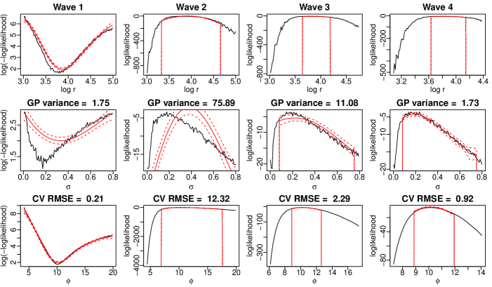
Figure 1: Diagnostics plots for the fitted GPs with one column per wave. A slice through the likelihood surface at $\theta=(3.8,0.3,10.0)$ is taken for each parameter in turn. The black line is the estimate of $l(\theta)$ (or $\log(-l(\theta))$ for the first wave) obtained from additional simulator runs. The red lines show the mean and 95% credible interval for the GP prediction of $l(\theta)$. Predictions in wave $i$ are only made in the not-implausible region $\Theta_{i-1}$.

The degree of conservatism of the criterion in ruling points implausible or not, is controlled by the choice of threshold $T$, and by the multiplier of $\sigma$ on the left-hand-side of the equation. For the examples considered below, the choice $T=10$ is found to provide a reasonable trade-off between accuracy and allowing sufficient space to be ruled as implausible, as $\exp(10)>10^{4}$, and so using the approximation $\pi(\theta|D)=0$ if $l(\theta)<l(\hat{\theta})-10$ causes only a small error in the approximation to the posterior.

3.2 Sequential approach

We aim to rule out an increasing proportion of prior input space $\Theta_{0}$ in a sequence of waves. Each wave involves extending the design, determining the implausible region, running the simulator at not-implausible points, building a new GP model, and running diagnostics. We start with ensemble $\mathcal{E}_{1}=\{(\theta_{i},\hat{l}_{M}(\theta_{i}))_{i=1}^{N_{1}}\}$ where $\{\theta_{i}\}_{i=1}^{N_{1}}$ are the first $N_{1}$ points from a Sobol sequence dispersed to fill $\Theta_{0}$ as described in Section 2.2. We denote the GP model fit to $\mathcal{E}_{1}$ by $\eta_{1}(\cdot)$.

The design is then extended by drawing $N_{2}$ additional points in $\Theta_{0}$. For each new point in the design we apply the implausibility criterion (3) using the mean and covariance function of $\eta_{1}$ to determine whether it is implausible or not, defining the not implausible region according to $\eta_{1}$, denoted $\Theta_{1}$. The simulator is then run at all the new design points that were ruled to be not implausible. Collected together with the points from $\mathcal{E}_{1}$ that were not implausible, this gives a new ensemble $\mathcal{E}_{2}$. We use $\mathcal{E}_{2}$ to build GP model $\eta_{2}(\cdot)$. Note that $\eta_{2}$ will only give good predictions for $\theta\in{\Theta_{1}}$.

For the i^th wave, we extend the design by a further $N_{i}$ points in $\Theta_{0}$. To judge whether $\theta$ is implausible, we first decide if $\theta\in\Theta_{1}$ using $\eta_{1}$, and if so, we then use $\eta_{2}$ to test if $\theta\in\Theta_{2}$, and so on. Parameter $\theta$ is only judged to be not-implausible if Equation (3) is not satisfied for all $i-1$ GP models fit in previous waves. It is necessary to use the entire sequence of GPs, as earlier GPs are only trained on the not-implausible region at that wave, and so are unable to usefully predict outside of this region, i.e., $\eta_{1}$ is unlikely to give poor predictions of $l(\theta)$ if $\theta\in\Theta_{0}\backslash\Theta_{1}$.

The motivation for this sequential approach is that the size of the not implausible region $\Theta_{i}$ decreases with each iteration, and more importantly, the value of $l(\theta)$ is less variable in $\Theta_{i}$ than in $\Theta_{i-1}$. This helps the GP model to achieve superior accuracy in later waves, and in particular, the variance of the predictions decreases (as there are more design points in the region of interest). While it is possible to reduce the threshold $T$ at each wave, we keep it fixed, and instead use the decreasing uncertainty in the improved GP fits to rule out increasingly wide regions of space.

The values of $N_{i}$ can be chosen either in advance, or by extending the design a point at a time until the number of not-implausible design points for the next wave is sufficiently large. To determine the number of waves needed, detailed diagnostics (Bastos and O’Hagan 2009) can be used to judge whether each GP model fit is satisfactory. For most problems, we have found 3 or 4 waves to be sufficient. Beyond this number, the need to iteratively use the entire sequence of GP models $\eta_{1},\ldots,\eta_{i}$ to judge implausibility becomes increasingly burdensome. For some problems, particularly if the prior support $\Theta_{0}$ includes regions with very large negative $l(\theta)$ values, it may be necessary to model $\log(-l(\theta))$ in the first wave, in order to cope with the orders of magnitude variation seen in the log-likelihood function. In these cases, the implausibility criterion will need to be suitably modified.

Once we have a GP model, $\eta_{I}(\cdot)$ say, that accurately predicts $l(\theta)$ within the not-implausible region $\Theta_{I-1}$, we can find the posterior distribution. We use a Metropolis-Hastings (MH) algorithm with random walk proposal. The acceptance step iteratively uses GPs $\eta_{1},\ldots,\eta_{I-1}$ to predict if the proposed parameter, $\theta^{\prime}$, is implausible. If $\theta^{\prime}\in\Theta_{I-1}$, then we use $\eta_{I}$ to predict $l(\theta^{\prime})$. We use a random realization (not just the GP mean) to account for the error in the likelihood prediction, and then use the MH ratio to decide whether to accept $\theta^{\prime}$ or not. Note that the MCMC does not require any further simulator evaluations.

Figure 2: The evolution of the experimental design through four waves of history matching (one column per wave). Each plot shows the projection of the design in the not-implausible region, $\Theta_{i-1}$, onto two dimensions. The proportion of the prior support $\Theta_{0}$ ruled out increases every wave and is reported in the figure. Note that the projection of the volume onto two dimensions acts to disguise the amount of space that has been ruled out.

4 Ricker model

The Ricker model is used in ecology to model the number of individuals in a population through time. Despite its mathematical simplicity, this model is often used as an exemplar of a complex model (Fearnhead and Prangle 2012, Shestopaloff and Neal 2013) as it can cause the collapse of standard statistical methods due to near-chaotic dynamics (Wood 2010). Although the model is computationally cheap, allowing the use of expensive sampling methods such as ABC, it is used here to demonstrate how GP-accelerated methods can dramatically reduce the number of simulator evaluations required to find the posterior distribution.

Let $N_{t}$ denote the unobserved number of individuals in the population at time $t$ and $Y_{t}$ be the number of observed individuals. Then the Ricker model is defined by the relationships

$$N_{t+1}=rN_{t}{\rm e}^{-N_{t}+e_{t}},\;Y_{t}\sim\operatorname{Pois}(\phi N_{t}),\;e_{t}\sim N(0,\sigma^{2})$$

where the $e_{t}$ are independent and the $Y_{t}$ are conditionally independent given the $N_{t}$ values. We use prior distributions $\log r\sim U[3,5],\;\sigma\sim U[0,0.8]$, and $\phi\sim U[4,20],$ and aim to find the posterior distribution $\pi(\theta|S(y_{1:T}))$ where $\theta=(\log r,\sigma^{2},\phi)$ is the parameter vector and $y_{1:T}=(y_{1},\ldots,y_{T})$ is the time-series of observations.

We apply the synthetic likelihood approach used in Wood (2010), and the GP-accelerated approach described here and compare their performance. We reduce the dimension of the data and simulator output, by using a vector of summaries $S(y_{1:T})$ which contain a collection of phase-invariant measures, such as coefficients of polynomial autoregressive models (described in Wood 2010). We use the Gaussian synthetic likelihood (Equation 2) and run the simulator 500 times at each $\theta$ in the design to estimate the sample mean and covariance ${\hat{\mu}}_{\theta}$ and ${\hat{\Sigma}}_{\theta}$. We use a simulated dataset obtained using $\theta=(3.8,0.3,10.0)$.

For the GP-accelerated inference we model $\log(-l(\theta))$ in the first wave, and $l(\theta)$ in later waves, and find that the best results are obtained using a total of four waves. We use a quadratic mean function for the GP model in the first three waves and a sixth order polynomial mean function in the final wave. After initial exploratory analysis to determine the rough shape of the log-likelihood function, we set the threshold value to be $T=3$ in the first wave (on the $\log(-l(\theta))$ scale), and $T=10$ for waves two to four, as these thresholds were predicted to lead to negligible truncation errors. The minimum value of the nugget variance for each GP was taken to be the variance of the estimate of $\log{\hat{\pi}}_{\mbox{{GABC}}}(S(y_{1:T})|\theta)$ (or $\log(-\log{\hat{\pi}}_{\mbox{{GABC}}}(S(y_{1:T})|\theta))$), estimated using 1000 bootstrap replicates of the sample mean and covariance matrix. Detailed diagnostic plots were used to guide these choices, a selection of which are shown in Figure 1. The accuracy of the GPs improves with each successive wave, which is reflected in the decreasing cross-validation errors (reported in the figure). Note that for earlier waves, it is only the ability to predict which regions are implausible that is important, not the absolute accuracy.

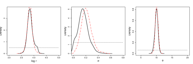
Figure 3: Marginal posterior distributions for the Ricker model. The solid black curve is the posterior obtained using the synthetic likelihood approach with $10^{5}$ MCMC iterations. The dashed red line is the posterior obtained using the GP-accelerated approach. The constant black dotted line is the prior. The synthetic likelihood posterior required $5\times 10^{7}$ simulator evaluations compared to only $3.5\times 10^{5}$ for the GP-accelerated approach.

Through the application of the thresholds, each wave of modelling rules out an increasing proportion of the prior support $\Theta_{0}$ as implausible. Figure 2 shows the design used in each wave, and the proportion of space ruled out. Wave one rules out 45% of $\Theta_{0}$, and by wave four, over 97% of space has been deemed implausible.

Figure 3 shows the posterior distributions estimated using the synthetic likelihood approach and the GP-accelerated approach. The GP-accelerated approach required a total of $3.5\times 10^{5}$ model evaluations. We ran the MCMC chain in the Wood method for $10^{5}$ iterations (which is probably too few), which required a total of $5\times 10^{7}$ simulator evaluations, 140 times more than required by the GP-accelerated approach. The posterior distributions for $\log r$ and $\phi$ are very similar, with the exception of an additional ridge in the posterior for $\log r$ which may be genuine, or may be an artefact of not running the synthetic likelihood MCMC for sufficiently long. The marginal posterior for $\sigma$ shows a small difference between the two methods. Estimating scale parameters is harder than estimating location parameters (Cox 2006), and it is usually when estimating scale parameters that the GP-accelerated approach has been observed to have poor accuracy.

5 Estimating species divergence times

We now examine a model used in evolutionary biology to estimate species divergence times using the fossil record (Tavaré et al. 2002, Wilkinson and Tavaré 2009). This model has an intractable likelihood function and has been used to demonstrate various advances in ABC methodology (Marjoram et al. 2003, Wilkinson 2007). The model consists of a branching process representing the unobserved phylogenetic relationships, which is randomly sampled to give a temporal pattern of fossil finds that can be compared to the known fossil record. We use data on primates (provided in Wilkinson et al. 2011), consisting of counts of the number of known primate species from the 14 geological epochs of the Cenozoic, denoted $\mathcal{D}=(D_{1},\ldots,D_{14})$. To model these data, a non-homogeneous branching process rooted with two individuals at an assumed divergence time of $54.8+\tau$ million years (My) ago is used (the oldest known primate fossil is 54.8My old). Informally, the parameter $\tau$ can be thought of as representing the temporal gap between the oldest primate fossil and the first primate, and is the key parameter of interest. Each species is represented as a branch in the process, with the branching probabilities and age distribution controlled by three unknown parameters $\rho,\gamma$ and $\lambda$. Once the branching process has been simulated, the number of species in each geological epoch are counted, giving values $\mathcal{N}=(N_{1},\ldots,N_{14})$. The fossil data, $\mathcal{D}$, are then assumed to be from a binomial distribution $D_{i}\sim\operatorname{Bin}(N_{i},\alpha_{i})$, with $\alpha_{i}=\alpha p_{i}$, where the $p_{i}$ are known sampling fractions reflecting the differing lengths of each epoch and the variation in the amount of visible rock. This gives five unknown parameters, $\theta=(\tau,\alpha,\rho,\gamma,\lambda)$, with primary interest lying in the estimation of the temporal gap $\tau$. We use uniform priors $\tau\sim U[0,100],\;\alpha\sim U[0,0.3],\;\rho\sim U[0,0.5],\gamma\sim U[0.005,0.015]$, and $\lambda\sim U[0.3,0.5]$ and try to find the posterior distribution $\pi(\theta|{\mathcal{D}})$.

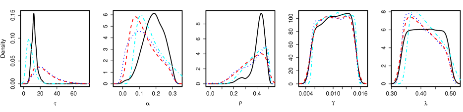
Figure 4: Marginal posterior distributions for the species divergence model. The solid black line shows the GP-accelerated approximation to the exact posterior. The dashed red line is from the rejection ABC approach. The dotted blue line is the GP-accelerated approximation to the ABC distribution. The dot-dash cyan line is from using a local-linear regression adjustment on the rejection ABC posterior.

The basic rejection ABC algorithm is simple to apply. We use the metric defined by Marjoram et al. (2003) with a tolerance of $\epsilon=0.1$, and generate 2000 acceptances from the algorithm given in Section 1, which required 13.6 million simulator evaluations (results shown as dashed red lines in Figure 4). For the GP-accelerated approach, we estimate the likelihood for each $\theta$ in our design by

$$\pi_{ABC}({\mathcal{D}}|\theta)\approx\frac{1}{M}\sum_{i=1}^{M}\mathbb{I}_{\rho(D,D^{\prime})\leq\epsilon}$$ (4)

where ${\mathcal{D}}^{\prime}$ is a simulated dataset. Due to the very low acceptance rate, we have to use a large value of $M$ to generate any acceptances, even when $\theta$ is near the maximum likelihood estimate. Approximately 50% of the prior input space led to no accepted simulations after $10^{4}$ replicates, which we dealt with by leaving these values out of the GP fit (alternatively, we can substitute a value less than $10^{-4}$ for the ABC-likelihood). An additional problem, is that the estimator of the ABC likelihood (Equation 4) has large variance, making the training ensemble a very noisy observation of the log-likelihood surface, which necessitates the use of a large nugget term in the Gaussian process. Surprisingly, we still find that the GP-accelerated approach is successful. Using two waves, with 128 design points in total, gives the results shown by the blue dotted lines in Figure 4. These results needed 1.28 million simulator evaluations, a factor of 10 fewer compared with the rejection ABC algorithm. The accuracy of these results is good, and can be improved further by increasing the value of $M$ and by refining the GP model of the log-likelihood surface.

The use of the discontinuous acceptance kernel (the 0-1 cutoff $\mathbb{I}_{\rho({\mathcal{D}},{\mathcal{D}}^{\prime})\leq\epsilon}$) in the ABC likelihood makes the log-likelihood surface difficult to model. Using a smooth GABC acceptance kernel $\pi({\mathcal{D}}|\mathcal{N})$, as in Equation (1), makes the estimate of the log-likelihood values less variable, and the surface easier to model. However, rather than present those results, we instead note that it is possible to approximate the exact posterior distribution in this case. The simulator consists of tractable and intractable parts. The distribution $\pi({\mathcal{N}}|\theta)$ is unknown and can only be simulated from, but the observation likelihood given the phylogeny is

$$\pi({\mathcal{D}}|{\mathcal{N}})=\prod_{i=1}^{14}\binom{N_{i}}{D_{i}}\alpha^{D}_{i}(1-\alpha)^{N_{i}-D_{i}},$$

and can be used to obtain log-likelihood estimates. Using this expression in a likelihood based inference scheme does not work well due to the extreme variance of the values obtained when ${\mathcal{N}}$ is drawn randomly from the model. Applying the GP-accelerated approach, is successful however. We used four waves, with 32, 78, 100, and 91 new design points in each wave, using a constant mean GP at each stage. At each design point $10^{5}$ simulator replicate were used to estimate $\pi({\mathcal{D}}|\theta)={\mathbb{E}}_{\mathcal{N}}\pi({\mathcal{D}}|{\mathcal{N}})$. The results are shown by the solid black lines in Figure 4. These distributions are an estimate of the posterior we would obtain if we could run ABC with $\epsilon=0$ (i.e., the true posterior). The GP-accelerated results differ from the ABC results (red line) because they approximate a different distribution, but they are consistent with our expectations. If one plots the ABC marginal posterior for $\tau$ for various values of $\epsilon$, then as $\epsilon$ decreases the posterior moves from a flat prior distribution, to an ever more peaked distribution with mass near smaller values of $\tau$. Also shown in Figure 4 (cyan dot-dashed lines) are the posteriors obtained using the local-linear regression adjustment proposed by Beaumont et al. (2002). This approach estimates the posterior we would obtain if we could set $\epsilon=0$ and can substantially improve the accuracy of rejection ABC. Note that the estimated posterior is somewhere between the rejection ABC posterior and the (possibly exact) GP posterior. As this curve is an extrapolation of the trend observed as $\epsilon$ decreases, we expect the GP-ABC posterior to be more accurate. We cannot quote any computational savings for the GP-accelerated approach, as to the best of our knowledge, it is impossible to obtain this (‘exact’) posterior distribution using any other approach.

6 Conclusions

For computationally expensive simulators, it may not be feasible to perform enough simulator evaluations to use Monte Carlo methods such as ABC at the accuracy required. GP-accelerated methods, although adding another layer of approximation, can provide computational savings that allow smaller tolerance values to be used in ABC algorithms, thus increasing the overall accuracy. Although the method is not universal, as it requires a degree of smoothness in the log-likelihood function, nevertheless, for a great many models this kind of approach can lead to large computational savings. The method requires user supervision of the GP model building and it is important that detailed diagnostic checks are used in each wave of the GP model building. Just as poor choices of tolerance, summary and metric in ABC can lead to poor inference, similarly, poor modelling and design choices can lead to inaccuracies in the GP-ABC approach.

Using GPs raises other computational difficulties, as GP training has computational cost $O(N^{3})$, where $N$ is the number of training points, with complexity $O(N)$ and $O(N^{2})$ for calculating the posterior mean and variance respectively. This cost means that this approach will not produce time savings if the simulator is very cheap to run. The cost of using GPs can be reduced to $O(M^{2}N)$ for training (and $O(M)$ and $O(M^{2})$ for prediction) by using sparse GP implementations (Quiñonero-Candela and Rasmussen 2005), which rely upon finding a reduced set of $M\ll N$ carefully chosen training points and using these to train the GP.

Finally, the method presented here can be extended in several ways. For example, the optimal choice of the number of simulator replicates, the error induced by thresholding the likelihood, and the location of additional design points have not been studied in detail. In conclusion, we have lost the guarantee of asymptotic success provided by most Monte Carlo approaches, in exchange for gaining computational tractability. Despite these drawbacks, GP-accelerated methods provide clear potential for enabling Bayesian inference in computationally expensive simulators.

References

- Barthelmé and Chopin [2014] S. Barthelmé and N. Chopin. Expectation-propagation for likelihood-free inference. J. Am. Stat. Assoc., to appear, 2014.
- Bastos and O’Hagan [2009] L. S. Bastos and A. O’Hagan. Diagnostics for Gaussian process emulators. Technometrics, 51:425–438, 2009.
- Beaumont [2010] M. A. Beaumont. Approximate Bayesian computation in evolution and ecology. Annu. Rev. Ecol. Evol. S., 41:379–406, 2010.
- Beaumont et al. [2002] M. A. Beaumont, W. Zhang, and D. J. Balding. Approximate Bayesian computatation in population genetics. Genetics, 162:2025–2035, 2002.
- Cox [2006] D. R. Cox. Principles of statistical inference. Cambridge University Press, 2006.
- Craig et al. [1997] P. S. Craig, M. Goldstein, A. H. Seheult, and J. A. Smith. Pressure matching for hydrocarbon reservoirs: a case study in the use of Bayes linear strategies for large computer experiments. In Case Studies in Bayesian Statistics, pages 37–93. Springer, 1997.
- Csilléry et al. [2010] K. Csilléry, M. G. B. Blum, O. E. Gaggiotti, and O. François. Approximate Bayesian computation (ABC) in practice. Trends Ecol. Evol., 25:410–418, 2010.
- Diggle and Gratton [1984] P. J. Diggle and R. J. Gratton. Monte Carlo methods of inference for implicit statistical models. J. R. Statist. Soc. B, 46:193–227, 1984.
- Drovandi et al. [2014] C. C. Drovandi, A. N. Pettitt, and A. Lee. Bayesian indirect inference using a parametric auxiliary model. In, submission, 2014.
- Fearnhead and Prangle [2012] P. Fearnhead and D. Prangle. Constructing summary statistics for approximate Bayesian computation: semi-automatic approximate Bayesian computation. J. Roy. Stat. Soc. Ser. B, 74:419–474, 2012.
- Gerber and Chopin [2014] M. Gerber and N. Chopin. Sequential quasi-Monte Carlo. arXiv:1402.4039, 2014.
- Kennedy and O’Hagan [2001] M. Kennedy and A. O’Hagan. Bayesian calibration of computer models (with discussion). J. R. Statist. Soc. Ser. B, 63:425–464, 2001.
- Marin et al. [2012] J.-M. Marin, P. Pudlo, C. P. Robert, and R. J. Ryder. Approximate Bayesian computational methods. Stat. Comput., 22:1167–1180, 2012.
- Marjoram et al. [2003] P. Marjoram, J. Molitor, V. Plagnol, and S. Tavaré. Markov chain Monte Carlo without likelihoods. P. Natl. Acad. Sci. USA, 100:15324–15328, 2003.
- Morokoff and Caflisch [1994] W. J. Morokoff and R. E. Caflisch. Quasi-random sequences and their discrepancies. SIAM J. Sci. Comput., 15:1251–1279, 1994.
- Quiñonero-Candela and Rasmussen [2005] J. Quiñonero-Candela and C. E. Rasmussen. A unifying view of sparse approximate Gaussian process regression. J. Mach. Learn. Res., 6:1939–1959, 2005.
- Rasmussen [2003] C. E. Rasmussen. Gaussian processes to speed up hybrid Monte Carlo for expensive Bayesian integrals. In Bayesian Statistics 7: Proceedings of the 7th Valencia International Meeting, pages 651–659, 2003.
- Rasmussen and Williams [2006] C. E. Rasmussen and C. K. I. Williams. Gaussian processes for machine learning. The MIT Press, 2006.
- Santner et al. [2003] T. J. Santner, B. J. Williams, and W. I. Notz. The design and analysis of computer experiments. Springer Verlag, 2003.
- Shestopaloff and Neal [2013] A. Y. Shestopaloff and R. M. Neal. MCMC for non-linear state space models using ensembles of latent sequences. arXiv:1305.0320, 2013.
- Sisson et al. [2007] S. A. Sisson, Y. Fan, and M. M. Tanaka. Sequential Monte Carlo without likelihoods. Proc. Natl. Acad. Sci. USA, 104:1760–1765, 2007.
- Tavaré et al. [2002] S. Tavaré, C. R. Marshall, O. Will, C. Soligo, and R. D. Martin. Using the fossil record to estimate the age of the last common ancestor of extant primates. Nature, 416:726–729, 2002.
- Toni and Stumpf [2010] T. Toni and M. P. H. Stumpf. Simulation-based model selection for dynamical systems in systems and population biology. Bioinformatics, 26:104–110, 2010.
- Toni et al. [2008] T. Toni, D. Welsch, N. Strelkowa, A. Ipsen, and M. P. H. Stumpf. Approximate Bayesian computation scheme for parameter inference and model selection in dynamical systems. J. R. Soc. Interface, 6:187–202, 2008.
- Vernon et al. [2010] I. Vernon, M. Goldstein, and R. G. Bower. Galaxy formation: a Bayesian uncertainty analysis. Bayesian Analysis, 5:619–669, 2010.
- Wilkinson [2007] R. D. Wilkinson. Bayesian inference of primate divergence times. PhD thesis, University of Cambridge, 2007.
- Wilkinson [2013] R. D. Wilkinson. Approximate Bayesian computation (ABC) gives exact results under the assumption of model error. Stat. Appl. Genet. Mo. B., 12:129–141, 2013.
- Wilkinson and Tavaré [2009] R. D. Wilkinson and S. Tavaré. Estimating primate divergence times by using conditioned birth-and-death processes. Theor. Popul. Biol., 75:278–285, 2009.
- Wilkinson et al. [2011] R. D. Wilkinson, M. E. Steiper, C. Soligo, R. D. Martin, Z. Yang, and S. Tavaré. Dating primate divergences through an integrated analysis of palaeontological and molecular data. Systematic Biol., 60:16–31, 2011.
- Wood [2010] S. N. Wood. Statistical inference for noisy nonlinear ecological dynamic systems. Nature, 466:1102–1104, 2010.