The large$-g$ observability of the low-lying energies in the strongly singular potentials $V(x)=x^{2}+g^{2}/x^{6}$ after their ${\cal PT}-$symmetric regularization

Abstract

The elementary quadratic plus inverse sextic interaction $V(x)=x^{2}+g^{2}/x^{6}$ containing a strongly singular repulsive core in the origin is made regular by a complex shift of coordinate $x=s-{\rm i}\varepsilon$. The shift $\varepsilon>0$ is fixed while the value of $s$ is kept real and potentially observable, $s\in(-\infty,\infty)$. The low-lying energies of bound states are found in closed form for the large couplings $g\gg 1$. Within the asymptotically vanishing ${\cal O}(g^{-1/4})$ error bars these energies are real so that the time-evolution of the system may be expected unitary in an ad hoc physical Hilbert space.

Keywords

quantum evolution; triple-Hilbert-space picture; strongly singular forces; regularization by complexification; strong-coupling dynamical regime; unitarity;

1 Introduction

Although the differences between the classical and quantum laws of evolution are deep, the search for their practical applications often proceeds in unexpectedly close parallels. For illustration one may recall the existence of certain parallelism between the principles and concepts of classical and quantum computing. One of the important ingredients in these developments may be seen in the recent thorough changes in the perception of quantum systems and of their theoretical description. In place of the traditional idea of preparation of a quantum wave function $\psi$ at time $t_{0}=0$ and of its exposition to measurement at time $t_{1}>0$, several innovations of the paradigm have emerged. In our present paper, specific attention will be paid to the underlying problem of the prediction of the results of the unitary evolution, based on the more or less routine solution of Schrödinger equation

$${\rm i}\partial_{t}\,\psi=H\,\psi\,$$ (1)

in which the Hamiltonian $H$ is NOT assumed self-adjoint, $H\neq H^{\dagger}$.

Review papers [1, 2, 3, 4] may be recalled for an exhaustive introduction into the underlying version of quantum theory in which the wave function $\psi$ is perceived represented, in parallel, in three alternative Hilbert spaces ${\cal H}^{(F,S,T)}$ where just ${\cal H}^{(S)}$ and ${\cal H}^{(T)}$ are assumed unitarily equivalent. The respective superscripts may be read as abbreviating “first”, “’second” and “third” Hilbert space. The “first” space is most important as being, in the textbooks, “favored” as the “friendliest” one.

Whenever one restricts attention to the most common one-dimensional kinetic plus local potential Hamiltonians $H=-d^{2}/ds^{2}+V(s)$, there rarely emerge any doubts about the choice of the first space in the form of the Hilbert space of the square-integrable functions of $s$, ${\cal H}^{(F)}\ \equiv\ L^{2}(\mathbb{R})$. In this context, Bender with Boettcher [5] were probably the first quantum theoreticians who sufficiently explicitly emphasized that such a choice of the representation space may be wrong and unphysical. In other words, the above reading of the superscript may happen to change into “false” [4].

Extremely persuasively, Bender and Boettcher illustrated the validity of such a claim by the demonstration of the reality of the spectrum of bound states (and, hence, of the possible unitarity of the quantum evolution after an ad hoc amendment ${\cal H}^{(F)}\to{\cal H}^{(S)}$ of the physical Hilbert space of states) even when generated by the following, manifestly non-Hermitian confining potential

$$V^{(BB)}(x)=({\rm i}x)^{\delta}\,x^{2}\,,\ \ \ \ \delta\geq 0\,.$$

We feel inspired by such a claim. We intend to extend the scope of the corresponding mathematics as summarized, e.g., in review paper [3] to the domain of applications in which the non-Hermitian confining potentials are allowed strongly singular.

For the sake of definiteness we shall pay our attention to the potentials exhibiting not only the left-right symmetry of the problem in the complex plane (also known as ${\cal PT}-$symmetry [2]) but also the following strong form of the central-repulsion property,

$$V(x)=g^{2}\,x^{-2-\gamma}+{\rm subdominant\ terms}\,,\ \ \ \ \ \gamma\geq 0\,,\ \ \ \ \ |x|\ll 1\,.$$ (2)

Our decision and project of study were motivated by the challenging available results as obtained, say, in refs. [6, 7] for the $\gamma=0$ weaker-singularity cases. One should add that at $\gamma=0$ the regularization proved comparatively easy as long as it could rely upon the centrifugal-force nature of the $\gamma=0$ repulsion. At the same time, one may expect that at $\gamma>0$ and $g^{2}>0$ the regularization of the singular spike may still be achieved by the same (in fact, by the Buslaev’s and Grecchi’s [6]) complex shift of the coordinate $x=s-{\rm i}\varepsilon$ in which the real shift parameter $\varepsilon>0$ is a constant while the value of $s$ is kept variable, $s\in(-\infty,\infty)$.

The text of our paper will be separated in section 2 (in which a specific model is chosen for our study), section 3 (in which we evaluate the low lying spectrum via a suitable perturbation technique) and discussions (section 4).

2 The model

The studies of the strongly spiked repulsive interactions (2) usually find motivation in perturbation theory [8] and in computational physics [9] as well as in field theory [10] and in descriptive and phenomenological contexts [11]. In our present paper devoted to the study of exactly solvable extremes we shall pick up one of the most elementary interactions

$$V(x)=x^{2}+\frac{g^{2}}{x^{6}}\,$$ (3)

where $\gamma=4$ and where the real coupling $g^{2}$ will be considered very large, $g\gg 1$. In addition, the related ordinary differential Schrödinger equation

$$\left[-\frac{d^{2}}{dx^{2}}+V(x)\right]\,\psi_{n}(x)=E_{n}\,\psi_{n}(x)\,$$ (4)

will be defined along the straight complex line of $x=x(s)\in\mathbb{C}$ where the parameter $s$ runs over the whole real domain, $s\in\mathbb{R}$. The distance $\varepsilon>0$ of this line from the real axis of $x$ will be kept fixed,

$$x=x(s)=s-{\rm i}\varepsilon\,.$$ (5)

The most common square-integrable bound-state solutions of our Schrödinger Eq. (4) in ${\cal H}^{(F)}\ \equiv\ L^{2}(\mathbb{R})$ will be required to satisfy the usual Dirichlet asymptotic boundary conditions,

$$\psi_{n}(x)=\psi_{n}[x(s)]=\phi_{n}(s)\to 0\ \ \ {\rm for}\ \ \ s\to\pm\infty\,.$$ (6)

Finally, the standard probabilistic interpretation of these states will be assumed achieved, in principle at least, via a change of the inner product in ${\cal H}^{(F)}$ (yielding a “standard” physical Hilbert space ${\cal H}^{(S)}$) or, if asked for, via a subsequent replacement of the second space ${\cal H}^{(S)}$ by its unitarily equivalent alternative ${\cal H}^{(T)}$. For more details the readers may check, e.g., ref. [4] in which we worked with superscript ^(P) (marking, in the inspiring context of ref. [1], the “primary” physical space) in place of the present, less sophisticated superscript ^(T) meaning just the “third” space.

The analyticity of our potential $V(x)$ in the complex plane of $x$ (with the exemption of the origin and infinity) implies immediately [12] that the wave-function solutions $\psi_{n}(x)$ of the ordinary differential Eq. (4) may be considered analytic in the complex plane of $x$, endowed with a properly chosen cut which would connect the origin with infinity. Naturally, for $\varepsilon>0$ we shall choose the cut starting at the origin and oriented upwards.

From the purely phenomenological point of view one of the key merits of our model (4) + (5) may be seen in our freedom of choosing any parameter $\varepsilon>0$. In the spirit of the standard oscillation theorems which hold for the complex linear differential equations of the second order [13] we know that due to the analyticity of the wave functions below the real line of $x$ the variations of the value of $\varepsilon>0$ will leave the spectrum unchanged. Thus, in particular, the choice of a very small $\varepsilon$ will enable us to approximate some of the “standard textbook” $\varepsilon=0$ bound-state wave functions by the not too different related solutions $\psi_{n}(x)$ of our present “regularized”, $\varepsilon\approx 0$ eigenvalue problem.

In contrast, the choice of a very large $\varepsilon$ will simplify the mathematics. We shall show below that the independence of the spectrum of the value of the shift parameter $\varepsilon$ may enable one to combine a useful predictive power of the model with certain friendly and constructive mathematical features.

3 Strong-coupling perturbation expansions

In our Schrödinger Eq. (4) the Hamiltonian is evidently non-Hermitian in $L^{2}(\mathbb{R})$ where, via Eq. (5), the symbol $\mathbb{R}$ represents the real line of variable $s$. This Hilbert space must be declared unphysical and “false”, therefore [4]. A deeper explanation of such an apparent paradox may be found in Refs. [1, 2, 14]. Its resolution is easy, in principle at least. An ad hoc redefinition of the inner products in $L^{2}(\mathbb{R})$ does the job. It makes the Hamiltonian, by construction, self-adjoint in the new, Hamiltonian-adapted Hilbert space ${\cal H}^{(S)}$ where the superscript ^(S) abbreviates the word “standard” [4].

Let us now return to the approximate solution of our differential Schrödinger eigenvalue problem (4) + (5) + (6), i.e., to the ordinary differential equation

$$\left[-\frac{d^{2}}{ds^{2}}+W(s)\right]\,\phi_{n}(s)=E_{n}\,\phi_{n}(s)\,,\ \ \ \ \ \ W(s)\ \equiv\ V[x(s)]=(s-{\rm i}\varepsilon)^{2}+\frac{g^{2}}{(s-{\rm i}\varepsilon)^{6}}\,$$ (7)

for the bound-state wave functions re-written in the equivalent form $\phi_{n}(s)\in L^{2}(\mathbb{R})$ and living on the real line of $s$. We shall restrict our attention to the strong-coupling dynamical regime where $g\gg 1$. We shall see that in such a dynamical regime one is permitted to use certain less usual perturbation expansions in a small parameter $1/g^{c}$ such that $0<c<1$.

The detailed description of the method may be found in Ref. [15] where the perturbation recipe has successfully been tested and found to work for complex-valued potentials. Here, it is only necessary to demonstrate that the presence of the repulsive barrier will not obstruct the applicability of such a perturbation-expansion technique.

3.1 Approximations using special values of $\varepsilon$

Perturbation theory as explained, e.g., in Ref. [15] tells us that its convergence to exact results cannot be guaranteed in general. Thus, one only has to use the formalism as a source of suitable asymptotic series and approximants. In this sense, the whole perturbation recipe will satisfy our present needs. Its essence can be summarized as based on several assumptions. Firstly, we shall require that the first derivative of our complex potential function will vanish at a certain complex value of $x=R_{m}$. This is our first stationarity requirement which reads $V^{\prime}(R_{m})=0$ and yields an elementary algebraic equation for all of the eligible complex points $R_{m}$,

$$2R_{m}=\frac{6g^{2}}{R^{7}_{m}}\,.$$

Such an algebraic equation possesses eight well-separated closed-form complex roots at which our potential is locally constant,

$$R_{m}=R\,e^{{\rm i}\,\pi\,(m-1)/4}\,,\ \ \ \ R=|3^{1/8}g^{1/4}|\gg 1\,,\ \ \ \ m=1,2,\ldots,8\,.$$

In Fig. 1 the positions of the roots $x=R_{m}$ in complex plane of $x$ are marked by the small numbered circles.

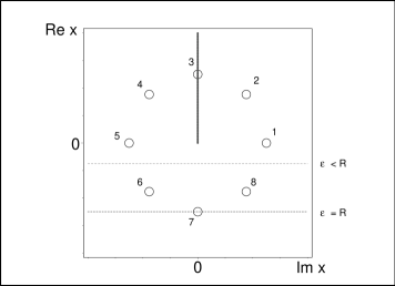
Figure 1: Positions of the eight roots $x=R_{m}$ (small circles) in complex plane of $x$ (with the thick-line cut oriented upwards). Two horizontal lines sample the eligible integration paths (5). The lower one which crosses the stationary point $R_{7}$ is exceptional, yielding the feasible single-well harmonic-oscillator approximation.

The well known second stationarity condition is the positivity of the second derivative of our potential $V(x)$ at the eligible stationary point $x=R_{m}$. Fortunately, irrespectively of the subscript $m$ we obtain the same real and positive value of this derivative,

$$V^{\prime\prime}(R_{m})=2+42\,\frac{g^{2}}{R^{8}_{m}}=2+42\,\frac{g^{2}}{3g^{2}}=16\,.$$

Thus, all of the eight points of stationarity are equally friendly from this point of view.

In the next step of our analysis we are free to select an optimal value of the optional complex shift $\varepsilon>0$ in integration path of Eq. (5). In Fig. 1 the thinner, upper horizontal line samples the generic case using a not too large shift $\varepsilon<R$. Along this line the shape of our complex potential function $V[x(s)]$ remains complicated and unfriendly to approximations (see its typical sample as presented in Fig. 2).

Figure 2: The rescaled real part ($\varrho^{-1}Re\{V[x(s)]\}$, symmetric curve) and rescaled imaginary part ($\varrho^{-1}Im\{V[x(s)]\}$, antisymmetric curve) of potential of Eq. (8) at $\varepsilon=R/100=1$ using the huge rescaling factor $\varrho=10^{15}$.

The thicker, lower horizontal line of Fig. 1 is chosen as crossing the seventh stationary point. The related shape of our complex potential function $V[x(s)]$ in sampled in Fig. 3. We immediately see that after such a special choice of $\varepsilon=R$, the shape of our potential $V[x(s)]$ resembles, very closely, the spatially symmetric harmonic-oscillator well near its minimum, with a very small admixture of an asymmetric imaginary component. Thus, an approximation of our interaction by a confining effective harmonic-oscillator potential may be expected very efficient at $\varepsilon=R$.

A detailed constructive proof of the latter expectation will be delivered in the next subsection. Before moving to this proof, let us briefly return to the other possibilities of the special choices of $\varepsilon<R$. First of all, we may exclude the use of the non-positive shifts $\varepsilon\leq 0$ as highly uncomfortable because the corresponding integration path would have to cross the cut or singularity.

In this sense the only remaining and apparently user-friendly alternative would be the choice of the integration line (5) with $\varepsilon=R/\sqrt{2}$. It would pass strictly through the pair of the left and right stationary points $R_{6}=x(-1/\sqrt{2})$ and $R_{8}=x(+1/\sqrt{2})$, respectively. Naturally, the resulting double-well problem (in which the two far-away wells are equally deep) is enormously complicated. In any case, it would not admit any easy perturbative treatment. Interested readers may find a deeper related methodical analysis in Ref. [16].

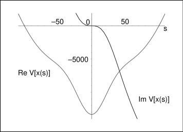
Figure 3: The real (symmetric) and imaginary (antisymmetric) parts of potential $V[x(s)]$ of Eq. (8) at $\varepsilon=R=100$.

3.2 Harmonic-oscillator approximation

Once we choose the path of Eq. (5) with $\varepsilon=R$ which crosses the only eligible candidate $R_{7}$ for a “useful” stationary point, we come to the conclusion that we satisfied all requirements and that we may finally apply the recipe of Ref. [15]. Let us now describe the results in full detail. In the first step let us reparametrize our potential,

$$V(x)=x^{2}+\frac{R^{8}}{3x^{6}}\,$$ (8)

and note that at large real $R$ and at the small complex shifts ${\rm i}\varepsilon=s-x(s)$ the shape and $s-$dependence of function (8) is wild and dominated by its singular part (cf. Fig. 2). At the large values of $\varepsilon\sim R$ the situation is different. The value of the complex function $V[x(s)]$ if dominated by its real part. Moreover, the latter real function of $s$ has a deep minimum at $x=-{\rm i}R$ (cf. Fig. 3). In such a case it makes sense to expand our complex potential near the stationary point $R_{7}\equiv-{\rm i}R$ in Taylor series. This yields the following complex power series in real variable $s$,

$$V[x(s)]=-\frac{4}{3}{R}^{2}+8{s}^{2}-{\rm i}{\frac{56}{3R}}{s}^{3}-\frac{42}{R^{2}}{s}^{4}+{\rm i}{\frac{84}{{R}^{3}}}{s}^{5}+\frac{154}{{R}^{4}}{s}^{6}-$$

$$-{\rm i}{\frac{264}{{R}^{5}}}{s}^{7}-\frac{429}{{R}^{6}}{s}^{8}+{\rm i}\frac{2002}{3{R}^{7}}{s}^{9}+\frac{1001}{{R}^{8}}{s}^{10}-\ldots\,.$$ (9)

The radius of convergence of the series is equal to $R$ and also the typical numerical factors of suppression of the next-order term remain large. Incidentally, the sequence of the polynomial truncations of the Taylor series may be found equal to the sequence of popular power-law interactions exhibiting ${\cal PT}-$symmetry [2]. Thus, we may truncate this series an insert the resulting polynomial interaction in our differential Schrödinger equation.

In the initial step of the construction we restrict our attention to the first two terms of series Eq. (9) and arrive at the exactly solvable model of the usual, real harmonic oscillator. This enables us to identify the low-lying spectrum of bound states of our model with the real energies given by the following closed formula,

$$E_{n}=-\frac{4{R}^{2}}{3}+(2n+1)\sqrt{8}+{\cal O}\left(\frac{1}{R}\right)\,,\ \ \ \ \ n=0,1,\ldots\,.$$ (10)

Finally, it is quite routine to show that all of the higher-order corrections to the potential in series Eq. (9) lead to the asymptotically vanishing corrections to the energies. We may summarize that within the limits of the first few orders of perturbation theory our model remains solvable. It is also worth noticing that the low-lying energy levels are perceivably negative and approximately equidistant.

4 Discussion

Certainly, our present result is perturbative so that the problem of the rigorous proof of the strict reality of the spectrum remains open. At the same time, the spectrum of energies of our present model is real within the precision offered by the perturbation series. The validity of such an observation may be further supported when we notice that the integrals representing the contribution of the odd powers in series (9) (i.e., of the purely imaginary corrections threatening to introduce also an imaginary component into the spectrum) vanish identically.

Naturally, whenever we are interested in the exact, non-perturbative energies our present arguments remain inconclusive (cf. also a few general relevant remarks on this topic in [17]). Our observation that the imaginary odd powers of $s$ in (9) cannot contribute to the Rayleigh-Schrödinger series only supports the reality of the spectrum in the limit $R\to\infty$.

Let us add that along the complex line of $x(s)=s-{\rm i}R$ also the analytic wave functions $\psi(x)$ of our model will coincide, with very reasonable precision, with the well known Hermite-polynomial wave functions of the linear harmonic oscillator with the spring constant $\omega^{2}=8$. This does not mean that from this information one could immediately deduce the behavior of the low-lying-state wave functions near $x=0$. The reason is that the propagation of the errors during the analytic continuation of wave functions is not under our control.

One of the serendipitous merits of interaction (3) is that we may easily write down the general solution of Eq. (4) in the complex vicinity of the origin,

$$\psi_{(c_{+},c_{-})}(x)\sim c_{+}\,e^{+g/(2x^{2})+\ldots}+c_{-}\,e^{-g/(2x^{2})+\ldots}\,.$$ (11)

This formula enables us to see that at $|x|\ll 1$, the two individual components of these solutions behave differently in the different small$-|x|$ complex Stokes sectors. The component $\exp({+g/(2x^{2})})$ will be dominant in the right (i.e., “first”) and left (i.e., “minus first”) rectangular wedges, where $|\arg x|<\pi/4$ and $|\arg(-x)|<\pi/4$, respectively, and vice versa. Although the latter observation may be read just as an $x\to 1/x$ image of the analogous statements valid for the more common large$-|x|$ Stokes sectors, the key novelty is that in the present context the distance of any acceptable, fixed complex integration curve ${\cal C}$ from the point $x=0$ is strictly greater than zero. The limiting transition to the origin would be a purely mathematical exercise, therefore.

This being said, it is still interesting to add a few formal comments on the consequences of the strongly singular character of our present potential function $V(x)$ at the unphysical point $x=0$. Firstly, any left plus right branches of a given low-lying wave function $\psi_{n}[x(s)]$ may be visualized as matching at $s=0$ (where $x=x(0)=-{\rm i}\varepsilon$, with $\varepsilon>0$ not necessarily optimal or even large). Secondly, due to the analyticity of these two functions (which will coincide at the physical bound-state energy) we may locally deform our straight complex line $x(s)$ and move the matching point upwards, closer to the origin. Keeping this deformation of the integration curve left-right symmetric, we may most simply get arbitrarily close to the origin along the negative imaginary axis. This means that we shall stay within the lower, “zeroth” Stokes’ wedge where $|\arg(-{\rm i}x)|<\pi/4$ so that it will be the minus-sign exponential component $\exp({-g/(2x^{2})})$ which will be growing and dominant in Eq. (11).

Clearly, our ${\cal PT}-$symmetric scenario is different from the current half-line constructions in which one strictly requires that $c_{+}=0$ and in which one approaches the origin from the left or right, i.e., within the minus first or first small$-x$ Stokes’ sectors. The analytic continuation of these solutions into the zeroth sector would lead to their unbounded growth near the origin. Conversely, one might impose the “anomalous” half-line-like boundary condition $c_{-}=0$ in the origin and expect that the corresponding new solutions will exhibit the exponential increase in the “usual” minus first and first small$-x$ Stokes’ sectors. Such a generalized form of analogy of our present $\gamma=4$ model with its exactly solvable $\gamma=0$ predecessor (involving, in the language of energies, the quick decrease of the low lying spectrum with the growth of the coupling $g$ and/or parameter $R$) would become only slightly more complicated for the larger exponents $\gamma$.

Acknowledgement

Discussions of the subject with Roberto Tateo and with several other colleagues are gratefully appreciated.

References

- [1] F. G. Scholtz, H. B. Geyer and F. J. W. Hahne, Ann. Phys. (NY) 213 (1992) 74.
- [2] C. M. Bender, Rep. Prog. Phys. 70 (2007) 947.
- [3] A. Mostafazadeh, Int. J. Geom. Meth. Mod. Phys. 7 (2010) 1191.
- [4] M. Znojil, SIGMA 5 (2009) 001, arXiv: 0901.0700.
- [5] C. M. Bender and S. Boettcher, Phys. Rev. Lett. 24 (1988) 5243; C. M. Bender, S. Boettcher and P. N. Meisinger, J. Math. Phys. 40 (1999) 2201.
- [6] V. Buslaev and V. Grecchi, J. Phys. A: Math. Gen. 26 (1993) 5541.
- [7] M. Znojil, J. Phys. A: Math. Gen. 33 (2000) 4561; M. Znojil, J. Phys. A: Math. Gen. 37 (2004) 10209.
- [8] E. M. Harrell, Ann. Phys., NY 105 (1977) 379; F. M. Fernández, Introduction to Perturbation Theory in Quantum Mechanics, CRC Press, Boca Raton (2001).
- [9] M. Znojil, Phys. Lett. A 158 (1991) 436; N. E. J. Bjerrum-Bohr, J. Math. Phys. 41 (2000) 2515.
- [10] V. V. Bazhanov, S. L. Lukyanov and A. B. Zamolodchikov, Adv. Theor. Math. Phys. 7 (2004) 711.
- [11] A. Kratzer, Z. Phys. 3 (1920) 289; L. D. Landau and E. M. Lifshitz, Quantum Mechanics (Pergamon, London, 1960), ch. V, par. 35.
- [12] Y. Sibuya, Global theory of a second order linear ordinary differential equation with a polynomial coefficient (Elsevier, 1975).
- [13] E. Hille, Ordinary Differential Equations in the Complex Domain (Wiley, 1976).
- [14] P. Dorey, C. Dunning and R. Tateo, J. Phys. A: Math. Theor. 40 (2007) R205.
- [15] M. Znojil, F. Gemperle and O. Mustafa, J. Phys. A: Math. Gen. 35 (2002) 5781; M. Znojil, Phys. Lett. A 374 (2010) 807.
- [16] M. Znojil and V. Jakubský, J. Phys. A: Math. Gen. 38 (2005) 5041.
- [17] E. Caliceti, S. Graffi and M. Maioli, Commun. Math. Phys. 75 (1980) 51; G. Alvarez, J. Phys. A: Math. Gen. 27 (1995) 4589.